Correlation indices : a new access method to exploit correlated attributes

Correlation Indices: a New Access Method to

Exploit Correlated Attributes

by

George Huo

Submitted to the Department of

Electrical Engineering and Computer Science

in Partial Fulfillment of the Requirements for the Degree of

Master of Engineering in

Computer Science and Engineering

at the

MASSACHUSETTS INSTITUTE OF TECHNOLOGY

May 2007

@ Massachusetts Institute of Technology 2007.

All rights reserved.

Author ...

...

...

...

...

Elýqrical Engineering and Computer Science

SMay

25, 2007

Certified by...u

.

-

...

. ...

Samuel Madden

Assistant Professor

Thesis upervisor

Accepted by....

...-.

...

'...-

...-..

...

Arthur C. Smith

Chairman, Department Committee on Graduate Students

,%KCH1VES

MASSACHUSETTS INS

E

OF TECHNOLOGY

OCT 0 3 2007

LIBRARIES

Correlation Indices: a New Access Method to Exploit

Correlated Attributes

by

George Huo

Submitted to the Department of Electrical Engineering and Computer Science on May 25, 2007,

in partial fulfillment of the requirements for the Degree of

Master of Engineering in Electrical Engineering and Computer Science

Abstract

In relational query processing, one generally chooses between two classes of access paths when performing a predicate lookup for which no clustered in-dex is available. One option is to use an unclustered inin-dex. Another is to perform a complete sequential scan of the table. Online analytical processing (OIAP) workloads often do not benefit from the availability of unclustered in-dices; the cost of random disk I/O becomes prohibitive for all but the most selec-tive queries. Unfortunately, this means that data warehouses and other OLAP systems frequently perform sequential scans, unless they can satisfy nearly all of the queries posed to them by a single clustered index [7], or unless they have available specialized data structures - like bitmap indices, materialized views, or cubes - to answer queries directly.

This thesis presents a new index data structure called a correlation index (CI) that enables OLAP databases to answer a wider range of queries from a single clustered index or sorted file. The CI exploits correlations between the key attribute of a clustered index and other unclustered attributes in the table. In order to predict when CIs will exhibit wins over alternative access methods, the thesis describes an analytical cost model that is suitable for integration with existing query optimizers. An implementation compares CI performance against sequential scans and unclustered B+Tree indices in the popular Berke-ley DB [22] library.

Experimental results over three different data sets validate the accuracy of the cost model and establish numerous cases where CIs accelerate lookup times by 5 to 20 times over both unclustered B+Trees and sequential scans. The strong experimental results suggest that CIs offer practical and substantial benefits in a variety of useful query scenarios.

Thesis Supervisor: Samuel Madden Title: Assistant Professor

Acknowledgments

I am indebted to my advisor, Sam Madden, for all of his invaluable support

throughout my graduate experience. The ideas in this thesis are primarily due to the discussions that we've had over the year. The process of learning how to conduct research, to teach, to think on a graduate level can go wrong in many ways. Sam has provided just the right balance of guidance and freedom while always keeping his students' best interests foremost, and I have grown all the more because of it.

I'd like to thank Adam Marcus for always being available to bounce ideas around with, from daily programming details to our SUL-Tree research. Hav-ing the opportunity to work with Adam taught me a great deal about how to collaborate effectively.

I thank anonymous referees who have provided many useful comments that

I've integrated into portions of the thesis.

Finally, I thank my family. I could not have made it without their support and sacrifice.

Contents

1 Introduction

1.1 Motivation for a new index structure

1.2 Overview of the correlation index . ...

1.3 Background and related work . . . . 1.3.1 Semantic query optimization . . 1.3.2 Unclustered index bitmap scans

1.3.3 Distinct value estimation . . . .

1.4 Contributions ...

1.5 Organization of thesis ... . . . . .

2 System Operation

2.1 Building correlation indices ... 2.2 Using correlation indices ...

2.3 Bucketing correlation indices ...

2.4 Discussion ...

3 Cost Model

3.1 Preliminaries ...

3.2 Cost of sequential scan . . . . 3.3 Cost of unclustered B+Tree

3.4 Cost of correlation index . . .

3.5 Discussion ... 31 . . . . 31 S . . . . . 32 S . . . . . 33 S . . . . . 36 . . . . 37 13 14 15 16 16 18 19 20 21 23 23 25 27 29

4 Prediction

4.1 Parameter collection ...

4.1.1 Computing the c.per_u parameter exactly ... 4.1.2 Approximating the cper_u parameter ...

5 Experimental evaluation 5.1 Implementation ... 5.1.1 Experimental setup . . 5.2 Indexing results ... 5.2.1 Synthetic results . . . 5.2.2 TPC-H results... 5.2.3 Census results... 5.3 Parameter calculation results 5.4 Summary of findings ... 47 . . . . 47 . . . . 48 . . . . 53 . . . . 53 . . . . 56 . . . . 60 . . . . 62 . . . . 64 6 Conclusion 41 42 43 44 67

List of Figures

2-1 Diagram illustrating an example CI and its use in a query plan.. 27

4-1 Algorithm to compute the model parameter c.peru for all pairs of attributes in table T ... 43 4-2 An illustration of alternative ways to calculate c.per_u statistics:

either by averaging the distinct salary count per state group, or by counting the number of distinct (state

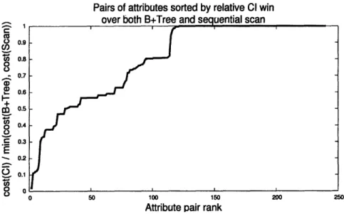
II

Smaller values represent more substantial wins. The plot sug-gests that we will see a win in roughly half of the 240 attribute

pairs. . ... 51

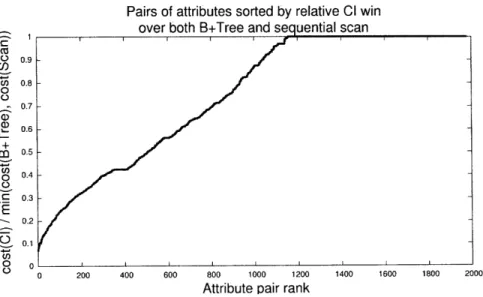
5-2 List of company attribute pairs sorted by expected win for a CI. Smaller values represent more substantial wins. The plot again suggests that we will see a win in roughly half of the 1980

at-tribute pairs... 52

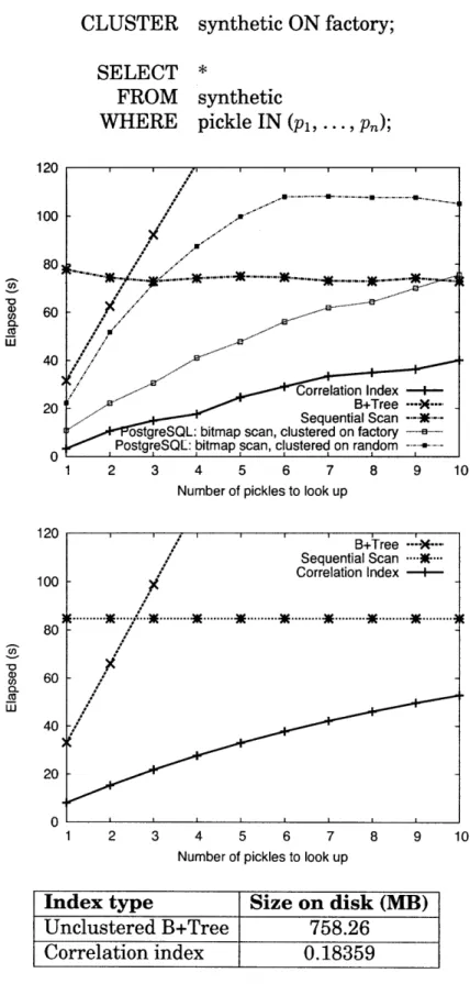
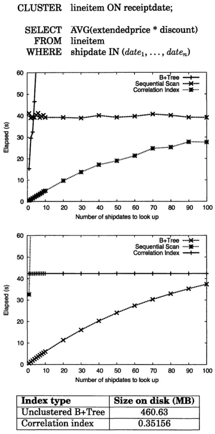
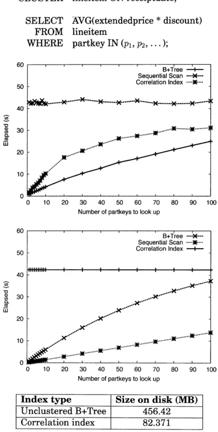
5-3 Time elapsed for queries over the pickle (unclustered) and factory (clustered) attributes in the synthetic table: experiment (above) vs. model (below). We also show the size of each index type on disk. 55 5-4 Time elapsed for queries over shipdate (unclustered) and

receipt-date (clustered) attributes in the lineitem table: experiment (above)

5-5 Time elapsed for queries over shipdate (unclustered) and

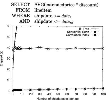
receipt-date (clustered) attributes in the lineitem table, now using a range

predicate. See Figure 5-4 for the model prediction. ... 58 5-6 Time elapsed for queries over partkey (unclustered) and

receipt-date (clustered) attributes in the lineitem table: experiment (above)

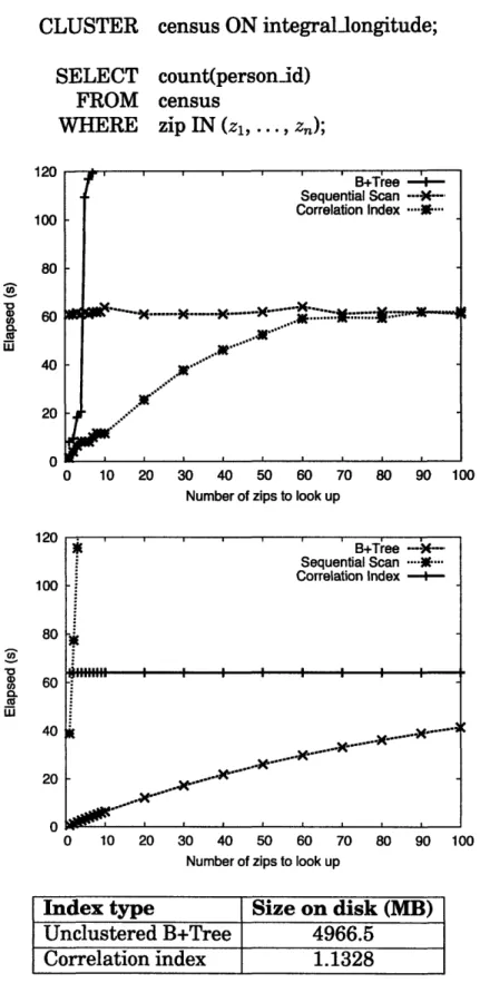
vs. model (below). We also show the size of each index type on disk. 59 5-7 Time elapsed for queries over zip (unclustered) and longitude

(clustered) attributes in the census table: experiment (above) vs. model (below). The longitude values have been bucketed into in-tegral bins from the original census data. We also show the size of each index type on disk ... 61 5-8 Time elapsed for six approaches that calculate cper_u values:

exact calculations in PostgreSQL and approximate calculations using Distinct Sampling with four different space bounds. .... 63

List of Tables

3.1 Table statistics used by the cost model. . ... 32 3.2 Hardware parameters used by the cost model. ... . . 32

5.1 Accuracy of Distinct Sampling lineitem estimates over four dif-ferent space bounds. Ratio error values closer to 1.0 are better. . 64

Chapter 1

Introduction

Database management systems (DBMSs) have become a central component of nearly all large software applications. One of the basic services provided by a DBMS is the ability to look up the records that satisfy a set of conditions in a user-specified predicate efficiently. Efficient lookups are fundamental to database systems not only because they support direct user queries, but also because they underlie many other database operations, such as aggregates and joins.

To implement such lookups efficiently, database systems employ indices over the columns in a table. An index is a data structure that is overlaid upon the table in order to be able to locate desired portions without reading the en-tire table. Traditionally, the B+Tree is the most common indexing structure in relational databases. Since an index represents some organization of the data, it is associated with the notion of a particular ordering of the records. We say that an index is clustered if the data are arranged on disk physically accord-ing to the order that the index represents. Unclustered indices lack many of the beneficial performance characteristics of clustered indices, especially as the size of the database table grows large. In particular, traditional unclustered in-dices are useful to look up specific values that occur infrequently, but queries that access more than a small fraction of the table become impractically slow.

1.1 Motivation for a new index structure

Online analytical processing (OLAP) workloads often do not benefit from the availability of unclustered indices. This is because queries in OLAP databases usually involve aggregation over regions of very large tables, instead of highly selective value lookups.1 The overhead of disk seeks to fetch the data pages pointed to by the leaf records in unclustered B+Trees will be higher than the cost to scan the table if even a small fraction of tuples in a table are accessed by a query. Clustered indices (and sorted files in some warehouse systems) perform better - beating sequential scans for many queries of even relatively low selectivity - but most database systems limit users to a single clustered index or sort order per table.

Unfortunately, this means that data warehouses and other OLAP systems will frequently perform sequential scans, unless almost all of the queries posed to them can be satisfied by a single clustered index [7], or unless specialized data structures - like bitmap indices, materialized views, or cubes - can be used to answer queries directly. In fact, Netezza, a popular appliance-based data warehouse, uses no indexing, relying exclusively on sequential scans be-cause it is hard to pick one index that will perform well for a range of ware-house queries.2 Although there are many attempts to optimize sequential scans (Netezza relies on special disk controllers and massive shared-nothing parallelism), ultimately any full table scan can be quite slow. An index struc-ture that leverages a particular table clustering to provide efficient lookups for more than one column, therefore, may yield benefits wherever systems cur-rently do no better than sequential scans.

1_{We adopt the convention that a highly selective query returns fewer tuples.} 2

1.2 Overview of the correlation index

This thesis introduces a new index data structure called a correlation index (CI) that allows OLAP databases to answer a wider range of queries from a single clustered index. The idea is to exploit correlations between the key attribute of a clustered index or sorted file (the "clustered attribute") and other "unclus-tered attributes" in the table. The simplest form of a correlation index is just a table that maps from each value u in the domain of an unclustered attribute Au to values of the clustered attribute A, that co-occur with u in some tuple in the database. Then, queries over Au can be answered by looking up the A, values co-occurring with u in the clustered index to find potentially matching tuples.3

If there is a high degree of correlation, then each u will co-occur with only a few clustered attribute values, such that answering queries over the unclus-tered attribute requires only marginally more lookups than would be required had a clustered index over Au been available. Because these lookups are per-formed directly on the clustered index, the matching tuples can be read directly from the index in sorted order in a very efficient manner (e.g., without perform-ing a disk seek for each additional tuple, as an unclustered index requires).

Obviously, this technique will not work for all attribute pairs. If there is no correlation between the clustered attribute and Au, each value in Au will map to many values in the index, and the efficiency of the approach will be quite low. Hence, one of the challenges of using correlation indices is determining when they will be effective and when they will be costly. This thesis presents an algorithm for determining the expected effectiveness of a correlated index based on simple statistics.

3

This is more general than a standard multicolumn index with the clustered attribute as the lead index column, since the user is not required to specify a predicate over the clustered attribute in the query.

1.3 Background and related work

In this section, we survey past work in semantic query optimization (SQO), soft constraints, and the bitmap scan access method related to the ideas presented in the thesis. We also provide background on sampling-based approaches to distinct value estimation, a technique we exploit in § 4.1.2 to calculate statistics for our cost model.

1.3.1

Semantic query optimization

One can view our work as an extension of certain optimization approaches from the field of semantic query optimization; there has been a long history of work in this area [5, 13, 16,21]. The basic idea is to exploit various types of integrity constraints (often expressed as rules [3, 4, 14, 15, 17, 20, 231) - either specified by the user or derived from the database - to eliminate redundant expressions in the query or to find more selective access paths during query optimization.

Past work in this area has studied several problems that bear some resem-blance to correlation indices. Cheng et al. [8] describe as one of their optimiza-tions predicate introduction (which was originally proposed by Chakravarthy et al [5]), in which the SQO injects new predicates in the WHERE clause of a query based on constraints that it can infer about relevant table attributes. Predicate introduction has traditionally focused on two approaches: index in-troduction and scan reduction. In the former case, a predicate is introduced naming a new attribute that may have an index available, which may then open up new possibilities for the query optimizer. In scan reduction, the intro-duction of range predicates can reduce the number of tuples that qualify for a join. These SQO techniques traditionally adopt a two-phase approach, where queries that are logically equivalent are first generated by query rewriting [8] and then submitted to the downstream query optimizer, from which the least expensive plan can be chosen. Thus, the effects of predicate introduction can be quite similar to those achieved by the CI for some clustered indices.

Gryz et al. [12] propose a technique for deriving what are called "check con-straints," which are basically linear correlations between attributes with error bounds (e.g., "salary = age * 1008 +/- 20000") and show that these relation-ships exist in data like TPC-H. They also look at a "partitioning" technique for string-valued attributes that finds cases where when an attribute X takes on a particular value v, some other attribute Y has a bounded range [a... b]. They show that these correlations can subsequently be exploited using predicate in-troduction over the detected constraint rules. Our approach generalizes Gryz et al.'s results in the context of indexing, because it can capture these relation-ships as well as non-linear relationrelation-ships (such as the fact that city names are correlated with states, even though one city may occur in many states).

Godfrey et al. [11] have looked extensively at discovering and utilizing "soft constraints" for semantic query optimization. They classify these integrity con-straints as absolute soft concon-straints, which hold with no exceptions in the cur-rent state of a database, and statistical soft constraints, which can have some degree of violation. They explain that such constraints can be used in query rewrite, query plan parameterization, and cardinality estimation in the opti-mizer's cost model for tighter guesses on selectivity factors.

However, the fact that their soft constraints capture only logical relation-ships between table attributes means that they must keep track of when the constraint no longer holds to invalidate the constraint or add violations to a special table that has to be unioned into the result of the query. They must account during every table update for the fact that the next change may inval-idate a particular soft constraint. CIs need not worry about this issue, because they do not explicitly represent logical constraints; rather, representing sets of co-occurring values makes CI maintenance simple over updates.

1.3.2 Unclustered index bitmap scans

Another indexing technique that is similar to correlation indices is the use of a bitmap scan to guide lookups over an unclustered index. One of the important reasons why CIs are able to achieve good performance is that they perform a subset of an in-order table scan on disk, avoiding unnecessary random I/O. We can make unclustered B+Trees behave in this way as well, using the following

modification.

Every value that we probe in the B+Tree returns a set of tuple or page offsets on disk. We map each of these offsets to a bitmap, and we union the bitmaps across multiple B+Tree probes to represent all of the disk offsets that we need to visit during one query. Such bitmaps can be generated on demand in memory. We can then scan the bitmap once to determine the sequence of off-sets to visit, which will naturally occur in order. For example, the PostgreSQL database system has implemented a bitmap scan access method in versions since 8.1. 4

Although the unclustered index bitmap scan makes no explicit mention of correlations, the scheme achieves good performance precisely when there are correlations between the lookup key and the clustered key - otherwise, the in-order schedule of resulting lookup pages still incurs random I/O costs and performs no better than a plain unclustered index. In this sense, the bitmap scan is a variation of the CI with different tradeoffs.

On one hand, a B+Tree identifies every matching tuple explicitly, so the optimizer has more information to work with when choosing a query plan. On the other hand, CIs are often far smaller than unclustered B+Trees. One of the

main motivations for developing the CI is to enable using many more indices at once than with unclustered B+Trees. Although we make the common modeling assumption in § 3.1 that indices fit in memory, this is less likely when dealing with many B+Trees simultaneously; as fewer levels of the search trees fit in

4

See discussion at http: //archives.postgresql.org/pgsql-performance/

memory, their performance will worsen sharply. Furthermore, we can tune the size of a CI freely using bucketing as we discuss in § 2.3, whereas a B+Tree's size is determined by the number of tuples it represents.

We present experimental results in § 5.2.1 to demonstrate our claim that bitmap scans perform well with a lookup column that is correlated to the clus-tered index, but that they degrade to a plain unclusclus-tered B+Tree when there are no useful correlations. Additionally, Chapter 5 describes the on-disk size of unclustered B+Trees versus CIs for each of our experiments, and we confirm that the CI is substantially smaller in every case.

1.3.3 Distinct value estimation

In § 4.1.2, we consider sampling-based approaches to measuring database statis-tics used by our cost model, including distinct value counts over single at-tributes and pairs of atat-tributes. The basic problem of predicting the number of distinct values in a column has seen extensive treatment in both the database community and the statistics community, where it is known as the problem of estimating the number of species (e.g. [21). All of the estimators proposed in the literature struggled with poor performance on input distributions with ei-ther high skew or low skew until a paper by Charikar et al. [61 proved a strong negative result that estimating the distinct count of a column within some small constant error requires reading nearly the entire table. The result is particularly decisive because it places few restrictions on the behaviour of the estimator, allowing any variety of random sampling and adaptive procedures.

To overcome this limitation of purely sampling-based approaches, Gibbons [10] proposed the Distinct Sampling algorithm that achieves far more accurate re-sults at the cost of one full table scan. While other work claimed that a small random sample is the only practical way to compute statistics over very large tables, Gibbons argues that one pass algorithms with fast incremental main-tenance are also scalable [10]. The one-pass approach to estimating distinct

counts was introduced by Flajolet and Martin [9], who proposed hashing dis-tinct values to a bit vector with specially tailored probabilities.

Since our approach to estimating statistics in § 4.1.2 relies only on distinct counts over attributes and pairs of attributes, it can also benefit from alterna-tive work in the area. For example, Yu et al. [24] look at estimating the number of distinct values across a set of attributes using histogram information main-tained within IBM DB2, instead of making additional passes over the data. We expect that future advances in the area will make our method even more practical and effective.

1.4 Contributions

In summary, correlation indices provide the potential to exploit correlations between attributes to allow clustered indices to be used as an access method for multiple attributes. This thesis describes the design and implementation of a correlation-indexing system, with the following key contributions:

* A description of the correlation index structure as well as algorithms for creating and querying it.

* A model of correlation index performance that allows one to predict how effective a CI will be compared to traditional database access methods (sequential scans and unclustered B+Trees). We show that this model is a good match for real world performance.

* A system design that is very low in complexity, one that can be integrated with existing access methods and query optimizers with little effort. * An evaluation of the effectiveness of CIs on several data sets, including

TPC-H data and data from the US Census Bureau. We show that CIs can outperform both unclustered indices and sequential scans by an order of magnitude on a variety of useful pairs of correlated attributes, and that

for real world data sets a quarter of attribute pairs can benefit from CIs

by more than a factor of two.

1.5 Organization of thesis

The remainder of this thesis is organized as follows.

* Chapter 2 overviews the operation of the system in more detail, including

how correlation indices are implemented and used.

* Chapter 3 describes an analytical model for estimating the cost to perform

a lookup in a particular correlation index, and it describes how to compare

against the expected costs of an unclustered index and a sequential scan.

* Chapter 4 describes a CI Advisor tool that collects statistics about

ex-pected CI benefit and actually evaluates the cost model to predict the

ben-efit of creating a given CI. The chapter also explores a practical

sampling-based approach to gathering and maintaining system statistics.

* Chapter 5 illustrates the benefits of CIs over several real-world

work-loads, and looks at their costs and overheads.

Chapter

2

System Operation

In this chapter, we describe the operation of correlation indices: how we iden-tify candidate CI attribute pairs, as well as how we physically store and main-tain CIs.

From a database client's standpoint, CIs work much like standard indices; they support customary update and query operations. For the database ad-ministrator, we provide a CIAdvisor tool to identify pairs of attributes that are likely to be good candidates for a CI. He can use this information to decide what clustered indices to build, as well as the associated CIs to build. By issuing a simple DDL command, he can add a CI linking a given attribute - the CI key

- to a clustered index. We describe the operation of the CI Advisor and how it computes the expected effectiveness of a CI in Chapter 4.

2.1 Building correlation indices

Suppose that a user wants to build a CI over an attribute T.A. of a table T, with a clustered index on attribute T.A,. The CI is simply a mapping of the form

u -+ S,, where u is a value in the domain of T.Au and S, is a set of values in the

domain of T.A, such that there exists a tuple t E T of the form (t.A, = u, t.A, =

c,...) _Vc E _{Sc. For example, if there is a clustered index on "product.state," a CI}

on "product.city" might contain the entry "Boston -+ {NH,MA}." The algorithm

for building a CI is shown in Algorithm 1. Once the administrator issues a DDL command to create a CI, the system scans the table to build the CI (line 2). As the system scans the table, it looks up the CI key value in the mapping and adds the clustered index key value to the key value set (line 3). A similar algorithm can be used for on-line insertions. Deletions, if needed, require the maintenance of an additional count of the number of co-occurrences with each value in the value set.1

input : Table T with attribute A, and clustered index over attribute Ac output: Correlation index C, a map from A, values to co-occurring Ac values 1 C +- new Map(Value -4 Set)

2 foreach tuple t c T do

/* Record the fact that t.Ac co-occurred with t.A, in the

mapping for t.A, */

3 C.get(t.A,).add(t.Ac) 4 end

5 return C

Algorithm 1: Correlation Index Construction Algorithm.

We physically represent the CI as a B+Tree keyed by the CI key, with the set of clustered index keys as the value for each record in the B+Tree. Whenever a tuple is inserted, deleted, or modified, the CI must be updated, as with a standard index. Because the CI is relatively compact (containing one key for each value in the domain of the CI attribute, which in our experiments occupy 1-50 MB for databases of up to 5 GB), we expect that it will generally reside in memory, although since it is a B+tree the database system is easily able to spill it to disk. We report on the sizes of the CI for several real-world attributes in our experimental evaluation in Chapter 5.

The clustered index over the table may be implemented either as a clustered B+Tree or as a simple sorted file. The CI benefits from the ability to scan the range of the table associated to a sort key efficiently. In a typical B+Tree im-plementation, while one can scan a series of matching tuples quickly one page at a time, it is still necessary to perform random disk seeks between pages.

1

It is not necessary for correctness to support deletions in CIs - in the worst case, they will result in scanning unnecessary values from the clustered index.

On the other hand, a sorted file can be stored contiguously on disk in order to provide optimal scan performance, but it does not support real-time updates as a B+Tree does. A static sorted file may be practical in many OLAP environ-ments, where updates are infrequent and can be batched until the sorted file is regenerated periodically. One possible trade-off is to use a clustered B+Tree implementation backed by a packed memory array [1], which provides a bound of 0(1 + (log2 N)/B) amortized memory transfers per update to a table with O(N) elements and a page size of B, and reduces sequential scan performance

by a factor of 2 at worst.

2.2 Using correlation indices

The API for the CI access method is straightforward; the CI implements a sin-gle procedure with the same interface as traditional access methods. It takes as input a set of values over the unclustered attribute associated to the CI, and it returns a list of tuples matching the desired set.

TupleList ci_lookup(Set unclustered_attrvalues);

When a query arrives that contains a predicate over an attribute for which

a CI is available, the database system will use the CI if the query optimizer

determines that it will be beneficial to do so. We did not implement a complete

query optimizer for our experimental evaluation, but we provide a cost model that we intend to be used by the query optimizer in Chapter 3. Using the cost model, the optimizer should pick a CI access path if it estimates that the access cost and selectivity will be less than some other access path for the same table. The optimizer should not pick a CI access path if another access path will provide an "interesting order" [19] that avoids sorts or reduces the cost of later operations in the plan outweighing the savings of using the CI.

Using a correlation index is straightforward. The basic lookup algorithm is illustrated in Algorithm 2. Given a range predicate p over a CI attribute, the

query executor looks up all of the records in the range in the CI (lines 2-4). It takes the union of all of the resulting clustered attribute value sets (line 3) and generates a sorted list of the clustered attribute values that need to be scanned (line 6). The executor looks up each of the matching values in the clustered index, in order (line 8). For each tuple that is returned, the executor checks to see if the tuple satisfies p (line 9), and if so, adds the tuple to the output set (line 10). This final predicate check is necessary because some values in the clustered index may not satisfy the predicate - for example, a scan of the states "MA" and "NH" to find records with city "Boston" will encounter many record from other cities ("Cambridge," "Somerville," "Manchester," etc.) that do not satisfy the predicate.

input : Correlation index C over attribute A,

Clustered index I on attribute Ac Range R over A,

output: List of tuples in R

1 indexKeys <- new Set() 2 foreach value r c R do

3 indexKeys <- indexKeys U C.get(r) 4 end

5 taps <- new TupleList()

6 sortedKeys <- inidexKeys.sortedList() 7 foreach k E sortedKeys do

/* I.lookupTuples returns tuples in I that have value k */ 8 foreach t e I.lookupTuples(k) do 9 if t.a E R then to taps.append(t) 11 end 12 end 13 end 14 return tups

Algorithm 2: Correlation Index Lookup Algorithm.

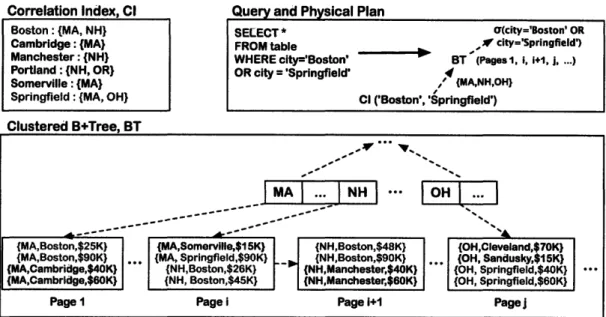
Figure 2-1 illustrates an example CI. Here, the user has a table with three attributes: state, city, and salary, with a clustered B+Tree on state. The ad-ministrator has created a CI on city. The CI maintains a correspondence be-tween each city name and the set of states it appears in. When a query with a restriction to the cities "Boston" and "Springfield" arrives, the system

gener-Query and Physical Plan

Clustered B+Tree, BT

MA _{.. NH}

" IOH ...

{MA,Boston,$25K}) (MA,Somerville,$15K) {NH,Boston,$48K) (OH,Cleveland,$70K)

{MA,Boston,$90K) ., {MA, Springfield,$90K) {NH,Boston,S90K) ,. (OH, Sandusky,$15K)

(MA,Cambridge,$40K) (NH,Boston,$26K) (NH,Manchester,$40K) (OH, Springfleld,$40K) ...

(MA,Cambridge,$60K) (NH, Boston,$45K) (NH,Manchester,$60K) (OH, Springfield,$60K)

Page 1 Page i Page 1+1 Pagej

Figure 2-1: Diagram illustrating an example CI and its use in a query plan. ates a physical query plan that uses the CI to identify the states that contain "Boston" and "Springfield" ("MA," "NH," and "OH"), and performs an in-order lookup on the clustered B+Tree to find the pages containing records from these states (1, 2, and 3 in our example). The tuples on these pages are fed to a se-lection operator, which returns only those tuples whose city matches "Boston" or "Springfield."

2.3 Bucketing correlation indices

The basic CI approach described in the previous section works well for at-tributes where the number of distinct values in the CI attribute or the clus-tered attribute is relatively small. However, for large attribute domains, the size of the CI can grow quite unwieldy (in the worst case having one entry for each tuple in the table). Keeping a CI small is important to keep the overhead of performing lookups low.

We can reduce the size of a CI by "bucketing" ranges of the CI attribute together into a single value. We can compress ranges of the clustered attribute stored in the CI similarly. A basic approach to bucketing is straightforward.

27 Boston: (MA, NH) Cambridge: (MA) Manchester: (NH) Portland :(NH, OR) Somerville: (MA)

Springfield : {MA, OH)

SELECT* O(city='Boston' OR

FROM table .if city='Springfield')

WHERE city='Boston' BT (Pages 1 i, i+1, j, ...)

OR city = 'Springfield' _,4

, {MANH,H}gfield')

CI ('Boston', 'Springfield')

For example, suppose we build a CI on the attribute temperature and we have a

clustered index on the attribute humidity (these attributes are often correlated

- with lower temperatures bringing lower humidities).

Suppose the unbucketed CI looks as follows:

{12.30_{C} -- {17.5%, 18.3%}}

{12.7°_{} -{18.9%,20.1%}}

{14.40C} - {20.7%.22.0%} {14.90C} {21.3%, 22.2%} {17.80C} - {25.6%, 25.9%}

We can bucket into 1OC or 1% intervals via truncation as follows:

{12 - 13C} {17 - 18%, 18 - 19%,20 - 21%} {14 - 150C} -

{20

{17 - 18C} - {25 - 26%}

Note that we only need to store the lower bounds of the intervals in the buck-eted example above. We omit a detailed algorithm for performing this trunca-tion, but we observe that the bucketing scheme could be as simple as taking an integer floor or as complex as arbitrary user-defined stored procedures.

The effect of this truncation is to decrease the size of the CI while decreasing its effectiveness, since now each CI attribute value maps to a larger range of clustered index values (requiring us to scan a larger range of the clustered in-dex for each CI lookup). In this thesis, we consider simple fixed-width binning schemes such as the one shown in the example above. 2 In § 5.2.3, we present

2_{Note that a poor bucketing can destroy correlations, since two CI values with very different}

clustered attribute sets may be placed into the same bucket. In this scenario, the CI must scan a large range of the clustered attribute space whenever we look up either CI attribute value. Hence, it is attractive for future work to look at adaptive binning techniques that merge together CI attribute buckets only when there is significant overlap in their clustered attribute sets.

experimental results to illustrate the effectiveness of the simple approach in one of our data sets.

2.4 Discussion

CIs capture the correlation between the CI attribute and the clustered at-tribute. If two attributes are highly correlated, each value of the CI attribute will co-occur in a tuple with only a few values in the clustered attribute, whereas if they are poorly correlated, the CI attribute will co-occur with many clustered attribute values.

Intuitively, correlated indices will be most effective when:

* There is a strict functional dependency between the unclustered attribute and the clustered attribute (that is, there is a many to one relationship, such that the unclustered attribute perfectly predicts the clustered at-tribute value). For example, in the United States, a zip code is a perfect predictor of a state. "Soft" functional dependencies should also perform well; for example, though a city name does not perfectly predict a state (since there is a Boston, M1A and a Boston, NH), city is often sufficient to predict state.

* The number of tuples across all clustered values to which an unclustered value maps is small. For example, in a nationwide database, city name is a good predictor of county, and there are many cities and counties. If a clustered index on county exists, it is likely that the index will also be useful for answering queries over city name, since the number of tuples for each county will not be large compared to the size of the database. As a counter-example, consider the TPC-H benchmark attribute "return-date," which indicates when a product was returned. It is perfectly cor-related with the attribute "returncode" that indicates whether or not a

product has been returned (returndate is null when no return has hap-pened, and non-null when it has). However, this correlation may not be useful, since the domain of returncode is so small that a very large frac-tion of the database has to be scanned whenever a clustered index on returncode is used.

It is also instructive to to compare the performance of CIs to unclustered B+Trees on the CI attribute. Clearly, using the correlation index will cause the system to read more tuples than it would read using an unclustered index. However, the CI can be much less expensive than an unclustered B+tree be-cause every tuple that is retrieved in an unclustered index requires a random disk I/O, whereas the CI scans all tuples with a given value from the clus-tered index, which keeps tuples with the same value together on the same disk page(s). We formalize this intuition in Chapter 3 where we model and compare the performance of unclustered B+Trees and CIs. 3

3It is interesting to note that it is possible to use an unclustered index in conjunction with a clustered index in much the same way we use a CI. This is true since if there is a correlation between the unclustered attribute and the clustered attribute, lookups of a particular value in the unclustered index will tend to be grouped onto a few pages of the clustered index. One way to view a CI is as a more compact representation of of an unclustered index used in this way.

Chapter 3

Cost

Model

So far in the thesis, we have given some intuition for when a CI might be less expensive than an unclustered index or a sequential scan; however, we have not provided a formal analysis for when this will be true. In this chapter, we describe an analytical cost model that we use to compare the absolute costs of the different access methods over an unclustered attribute. In particular, we examine an unclustered B+Tree index, a full table scan, and a CI over a given pair of attributes. Our goal is to compute the expected runtime of a lookup given parameters characterizing the underlying hardware and basic statistics extracted from the data.

3.1 Preliminaries

In the following discussion, we assume a table with attributes A, and A,. The field A, serves as the clustered attribute for the table, and the field A, is the unclustered attribute upon which we query. Our model assumes that the table is stored as a heap file sorted on A, for fast sequential scans. Thus, to read all of the tuples corresponding to a clustered attribute value, we look up the file offset corresponding to the value and perform a disk seek. We then read the relevant tuples sequentially.

Table 3.1: Table statistics used by the cost model.

tups-per-page Number of tuples that fit on one page.

c_tups Average number of tuples appearing with each Ac value.

c-per_u Average number of distinct Ac values for each Au value.

totaltups Total number of tuples in the table.

nlookups Number of A, values to look up in one query.

queries have not recently executed. We do not charge the B+Tree or CI access methods for reading index pages, since the upper levels of an active index are likely to be cached in a warm system. We assume that the cache initially holds none of the table pages. After a page has been accessed once, we do not charge an operator to read it a second time.

In Table 3.1, we summarize the statistics that we calculate over each table. Additionally, in Table 3.2, we describe the hardware parameters we use, along with typical values measured on our experimental platform. Most model pa-rameters are straightforward, and we describe in Chapter 4 how to measure them automatically.

We assume that all of the access methods are disk-bound. We do not model the CPU costs associated to traversing a B+Tree nor filtering tuples in the CI, and the cost of the sequential scan is independent of the number of values we look up. Through CPU profiling of the implementation that we present in Chapter 5, we have validated that our assumption is reasonable.

3.2

Cost

of sequential scan

The sequential scan operator is the simplest access method to model. Given our model parameters, the number of pages in a table is total_tups/tups_per_page.

The cost of scanning a table is then

costsc = (sequential page cost) ( totaltups tupsper-page)

We note here that our model is oblivious to external factors such as disk fragmentation. We found that this may not be true, for example, with sequen-tial scans over tuples stored in Berkeley DB B+Tree files, which tend to be highly fragmented. This factor is entirely implementation-specific, so we do not attempt to model it and we control for it in our experiments by defragmenting each file before a query begins.

3.3

Cost

of unclustered B+Tree

In our model, every tuple read via an unclustered B+Tree index causes a ran-dom seek. Given that we expect utups tuples to be associated to each Au value, the basic cost of looking up n-lookups values using a B+Tree is simply

cost btree = (random seek _cost) (u-tups) (n _lookups)

However, we must be careful about charging too much when the same pages are likely to be accessed more than once.

In addition to modeling the behavior of random disk accesses, it is important to model the effect of the database system's buffer pool on access costs. We have chosen not to adopt a complicated caching model, which would obscure the primary effects that we wish to compare between unclustered B+Trees and CIs. Instead, we propose the following simple model that captures the first-order effects of the buffer pool.

Suppose at the beginning of a query that we have a buffer pool of unlimited size that has cached none of the heap pages storing table data. The first time we request any heap page, we incur the cost of one disk read; subsequently, requests for that page are free. Furthermore, assume that the B+Tree samples

pages uniformly at random from the heap with replacement.

Theorem 3.3.1. Under our caching model, the expected number of cache hits

after p requests in a file with n pages is

(3.1)

Proof Let Hi be an indicator variable that is 1 if request i hits the cache, and

let Ci be a random variable representing the number of pages in the cache immediately before request i. Then, the expected number of cache hits after p requests is EP, Hi. Manipulating this expression, we have:

P[ ]

E Hi

=

ZE[H

]

P

=ZZ

XPr(Ci = x)

Now, let us consider E[Ci], the expected number of pages in the cache at request

i. We wish to define a recurrence by relating the number of cached pages at step i to the number of cached pages at step i - 1. Let us denote the page requested

at step i by Ri. The number of pages in the cache will increase by one after a request iff that request misses the cache. Using this fact, by our model we have

34

(n - 1)p+_l

1+ p - n + -(-1P+

that

E[C1] = E[Ci-1] + P(RE misses the cache)

= E[Ci•1] + 1 - P(Rz hits the cache)

= E[Ci_1] +

1-n

= 1+ (n n1)E[

This recurrence has the straightforward solution

E[Cj]

=

-n

((

i

72)

Substituting this expression back into our original calculation, we conclude that P[ H

E =1

-n (

n-1

Finally, we incorporate the caching model into our expected B+Tree cost.

Finally, we incorporate the caching model into our expected B+Tree cost. n- 1

Instead of performing a random seek for each result tuple, we now perform one random seek only for each predicted disk read:

disk.reads = (utups) (nlookups) - cache hits costbtee = (random_seek _cost) (disk _reads)

We have assumed that each tuple read via an unclustered B+Tree index causes a random seek - for example, if values were inserted in the B+tree in some secondary sort order. If the database system has more information about the distribution of values across pages (e.g. via histogram statistics in the system catalog), it can take the statistics into account by varying the

ran-dom-seekcost for B+Tree operations.

3.4 Cost of correlation index

Having developed a general caching model in the previous section, we now describe the expected cost of a correlation index lookup. We will see that we can apply our previous caching result almost directly, with one simple modification for the CI access pattern.

Suppose as usual that the CI has a set of A, values to look up. For each A, value, we must visit c.peru different clustered attribute values. We will need to perform one random seek to reach each of these clustered attribute values, followed by a scan of all of the pages for that A, value. In terms of the parameters we are given, the number of pages for a given Ac value is

ctups/tups_perpage.

Now, we must take into account cache hits as before. The key difference while modeling the CI is that our former assumption of an access pattern sam-pling pages uniformly at random is false - each clustered attribute that we visit results in the CI reading a contiguous segment of pages (a "superpage"),

To modify our assumption, suppose we know that there are cpages =

ctups/tups perpage pages associated to each clustered attribute value. Then,

there are now only total _tups/tups_per_page/cpages superpages in the file, and we can apply our caching model to the superpages.

Summarizing our ideas, the expected number superpages that we visit is determined by the following expressions.

c_tups

cpages =

tupsper.page

n_superpages = (n

n_lookups) (cper_u)

-

cache_hits

Combining these expressions, the overall cost of a CI lookup is cost ci = (n _superpages) (random_seek_cost

+ (sequentialpage_cost) (cpages))

Similar to our assumption that each secondary B+Tree tuple causes a ran-dom seek, we choose not to model the overlap between the sets of Ac keys as-sociated to two particular Au values. In other words, if one A, value maps to n different A, values on average, then it is not true in general that two Au values map to 2n different Ac values. Our model may overestimate the number of A, values involved, and thus the cost of CI.

We have chosen to omit this statistic in the interest of a simpler model, but we observe here that the desired overlap can easily be measured from the table by sampling pairs of uncorrelated attribute values and computing the average overlap between the resulting sets of Ac values.

3.5 Discussion

We have presented a series of expressions that estimate the cost of lookups us-ing a sequential scan, an unclustered B+Tree, and a CI. While the expressions

are fairly simple, they involve disparate sets of parameters that make compari-son inconvenient. For this reacompari-son, we now provide some intuition for situations where a CI might be more or less expensive than a sequential scan or B+Tree.

Sequential scan: The CI access pattern can be thought of as a subset of a

se-quential scan - that is, the CI will always read segments of a file in the same order as a sequential scan would, but it will jump over some stretches of the file. The CI reads fewer tuples than the sequential scan, but it still incurs some cost from disk seeks. Thus, there exists a trade-off in our model between re-ducing the number of tuples that the CI reads and the number of extra seeks that it performs.

In general, the CI will beat a sequential scan when the selectivity is high, and it is reasonable to expect the performance of CI to degrade to that of the sequential scan when the selectivity becomes low (indeed, the CI access pattern becomes more and more like a sequential scan). However, it is worth noting that it is possible for the CI to be more expensive than a sequential scan by a constant factor for low selectivities, because there is a noticeable overhead associated with seeking (even if the seeks are in-order and do not skip large distances in the file).

Unclustered B+Tree: The difference between the performance of CIs and B+Trees

is less straightforward to grasp. There are essentially two trade-offs that may apply to a particular query situation.

First, suppose that c_tups is low; that is, the average number of tuples for each clustered attribute value is small. This suggests that the number of irrel-evant tuples that a CI reads will not be too large, because the CI will not fall into reading long segments of the file with only a few matching tuples.

In this case, the primary trade-off occurs between the utups and c_peru parameters. If u_tups is high, then the B+Tree will incur a higher cost by performing a random seek for each A, value. On the other hand, if cperu is high, then the CI will need to visit a large number of clustered attribute

locations in the file (each of which also costs a random seek).

Now, suppose that cups is high, so that each A, clustered attribute value

that the CI must visit is very expensive. In this case, it is important for the CI

not to have to visit very many A, values, or rather that the correlation between

A. and Ac values be high.

Given that ctups is high, the scenario most favorable to the CI occurs when

a given A, value maps to a single A, value, but where there are many tuples

scattered throughout that Ac superpage matching A,. The CI needs merely to

scan the single superpage, while the B+Tree must perform numerous random

probes within that superpage.

The scenario least favorable to CI occurs when there are only a handful of

tuples in the file matching the A, value, but where each of the tuples co-occurs

with a different clustered attribute value. Now, the CI must scan and discard

a large number of irrelevant tuples while the B+Tree can seek to the desired

pages directly.

Chapter 4

Prediction

The introduction of a new access method to the database system complicates the job of the database administrator. Judging when a correlation index will be beneficial for a given pair of attributes is difficult to do by hand. Indeed, the administrator would need to weigh his estimation of the domain sizes of each attribute against the overall size of the table and the cost of random disk I/O.

Fortunately, given the analytical model that we have developed, we can fully automate the process of predicting when CIs will be useful. In our imple-mentation, we built a CI Advisor tool that scans existing database tables and calculates the statistics needed by the cost model. Given these statistics and measurements of underlying hardware properties, the CI Advisor can predict accurately each pair of attributes that would benefit from a CI. Presented with this information, the database administrator need only choose pairs from the list that the application is likely to query.

Since the CI Advisor computes sufficient statistics to evaluate the cost model for any set of parameters, our implementation is capable of generating plots of the expected query performance over each of the three access methods. In Chapter 5, we present the plots predicted by the CI Advisor alongside our em-pirical results. Our results suggest that the CI Advisor produces accurate esti-mates.

4.1 Parameter collection

In order to form predictions based on the cost model, the CI Advisor must refresh the statistics listed in Figure 3.1 based on the current state of the database. These include cltups and cper_u, which are based on counts of the number of distinct values in the database. We first present a naive procedure to gather the statistics. The approach is straightforward to understand, and it is possible to compute the relevant aggregates using standard SQL queries within the database system itself. Such aggregate queries may however be im-practically expensive, however, and we present a sampling-based approach in

§ 4.1.2 to reduce the overhead of parameter collection by an order of magnitude

or more. We present experimental results in § 5.3 to contrast the effectiveness of the different approaches.

The parameter total_tups is simply a count of the number of tuples in the table, which we expect the DBMS to maintain already as a routine statistic. The parameter c_tups can also be computed as totaltups divided by the num-ber of distinct values in Ac, which is also routinely maintained in the system catalog. Furthermore, the average number of tupsper page can be determined easily by dividing the size of a database page on disk by the average width of a tuple.

Our model further relies on the sequentialpagecost and randomseek _cost

-parameters that are characteristics of the underlying disk. Instead of depend-ing on the user to supply these values, our implementation measures them directly by creating large files on the target filesystem and reading them via sequential and random access patterns. Since the hard disk parameters asso-ciated with a given table file can change over time (due to external factors such as disk fragmentation), we recommend that these parameters be refreshed pe-riodically to reflect the current state of the file.

4.1.1 Computing the c-per_u parameter exactly

The c.peru parameter, the average number of distinct clustered key values for

each lookup key value, is the chief statistic that captures degrees of correlation

within our model. Unfortunately, it is also by far the most expensive statistic

to compute exactly.

For the purposes of the CI Advisor, we must compute one c.per_u value for

each ordered pair of fields in the table. To compute the set of cperu

param-eters for each pair, we perform the queries listed in Figure 4-1. For each

at-tribute G in the table T, we issue one SQL statement that groups by G. In

the inner query of the statement, the C, through C, terms produce the distinct

counts across every other attribute of T within each group of G. Then, the

outer query takes the average number of distinct counts across all groups of G

for each attribute. The final output values are the average counts of distinct Ai

values for each G value. 1

Note that each count(DISTINCT ... ) term must be processed using a

sepa-rate sort or hash operation. Thus, the number of disk output buffers in general

across all cper_u pairs will be quadratic in the number of columns, and the

performance is likely to be impractical in real applications.

foreach attribute A E T:

select avg(counts.C1), ..., avg(counts.OC)

from (select count(DISTINCT A,) AS C1,

count(DISTINCT A,) AS C,

from T

group by A) as counts

Figure 4-1: Algorithm to compute the model parameter cper_u for all pairs of

attributes in table T.

1In terms of c-peru _{parameters, the group-by attribute G corresponds to the unclustered}

4.1.2 Approximating the cper_u parameter

Our initial approach to computing exact c_per_u statistics is expensive. Previ-ous works in semantic query optimization tools, which need to gather similar statistics, have proposed analogous schemes. For example, Gryz et al. [12] sug-gest applying a linear regression statistic model over all comparable pairs of fields in each table, which they can achieve only by a similarly brute-force

ap-proach.

Since intensive aggregates are expensive for very large databases, it is nat-ural to ask if we can achieve reasonable estimates for our desired statistics via a sampling-based approach over our tables. If we can reduce the cost of deter-mining the distinct counts of each field as well as the cper_u counts, then we can reduce the execution time of the CI Advisor and improve the staleness of the cost model used for query optimization.

Before we turn to approximation, we observe that the naive approach com-puted the distinct count over A, values for each Au group, and subsequently took the average of the per-group distinct counts. Since we desire only the average value as the output, computing the distinct count for each group indi-vidually is in fact unnecessarily expensive. We now present a simplification for the exact algorithm.

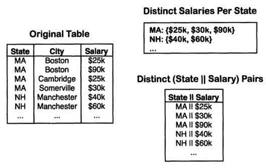
Consider the example of calculating the average number of distinct salaries per state in Figure 4-2. As opposed to counting the number of distinct salaries directly (shown above), we could alternatively enumerate the distinct pairwise values (shown below) and divide by the number of groups. In this case, there are five distinct (state II salary) pairs across two state groups, so the cperu

count is 2.5. Stating our observation more generally, let us write the number of distinct values over a pair of attributes A, and Aj within a set of tuples T as DT(Aj, Aj) and the number of distinct values over a single attribute as DT(Ai).

Original Table

State City Salary

MA Boston $25k MA Boston $90k MA Cambridge $25k MA Somerville $30k NH Manchester $40k NH Manchester $60k

-..

...

I

...

j

Distinct Salaries Per State

MA: {$25k, $30k, $90k} NH: {$40k, $60k}

Distinct (State II Salary) Pairs State I! Salary MA II $25k MA 11 $30k MA II $90k NH II $40k NH II $60k

Figure 4-2: An illustration of alternative ways to calculate cperu statistics: either by averaging the distinct salary count per state group, or by counting the number of distinct (state jI salary) pairs.

Then, it is clear that

EaEgroups

ofAo

Da(Ac)

DT(A),

Ac)

In other words, instead of computing each cper_u value explicitly using an average over an expensive grouping aggregate operation, we can alternatively calculate distinct counts for each single attribute and each attribute pairs. Then, we simply divide the distinct counts as necessary to derive each c-peru value.

Now, we describe how to apply a sampling-based approach to improve the performance of our scheme for approximate answers. In § 1.3.3, we discussed the Distinct Sampling algorithm presented by Gibbons. Of particular interest to our problem, Distinct Sampling can provide highly accurate estimates of dis-tinct counts (experimentally, often within 10%) over numerous table attributes using relatively small, constant space bounds and a single table scan. We refer the reader to [10] for a full presentation of the algorithm.

complexity, the Distinct Sampling algorithm is well-suited to computing dis-tinct value estimates over the entire set of target attributes in one pass. Thus, in order to approximate distinct count statistics efficiently, we create one Dis-tinct Sampling instance for each target attribute and attribute pair. To derive the actual c_per_u values used by the model, we calculate DT(Au, Ac)/DT(Au) as

necessary.

Our revised procedure for computing c.per_u estimates achieves a high de-gree of accuracy while reducing the calculation runtime by over an order of magnitude, which we demonstrate experimentally in § 5.3. While the num-ber of Distinct Sampling instances is still quadratic in the numnum-ber of columns, each instance requires only a small, constant amount of state and the entire operation is likely to fit in memory. Furthermore, it has the key property that the D(Aj) and D(Ai, Aj) values supplied by each Distinct Sampling instance can be maintained efficiently online in the presence of insertions. It is now possible, therefore, for the DBMS to maintain up-to-date c_peru estimates for use by the planner during query optimization, instead of relying on one-time statistics that are computed periodically and become stale.

Chapter 5

Experimental evaluation

In this section, we present an experimental validation of our results. We have developed an analytical model and an accompanying tool to identify cases where CIs are useful; however, we have not yet shown that such cases routinely exist. Additionally, we would like to argue that CIs are likely to be useful in a large fraction of pairs of attributes across a given table. The goals of our experiments are thus threefold:

1. to validate the accuracy of our analytical model

2. to establish that useful correlations are reasonably common in large data sets

3. to demonstrate that there exist cases where CIs win over both B+Trees and sequential scan and to measure the extent of that benefit.

5.1 Implementation

To conduct our experiments, we have completed an implementation of correla-tion indices that is suitable for comparison against Berkeley DB B+Trees and full table scans. We have chosen Berkeley DB as a low-overhead B+Tree library to avoid conflating unrelated system effects in a full DBMS.