HAL Id: hal-01805931
https://hal.archives-ouvertes.fr/hal-01805931
Submitted on 8 Oct 2020
HAL is a multi-disciplinary open access
archive for the deposit and dissemination of
sci-entific research documents, whether they are
pub-lished or not. The documents may come from
teaching and research institutions in France or
abroad, or from public or private research centers.
L’archive ouverte pluridisciplinaire HAL, est
destinée au dépôt et à la diffusion de documents
scientifiques de niveau recherche, publiés ou non,
émanant des établissements d’enseignement et de
recherche français ou étrangers, des laboratoires
publics ou privés.
sub-grid-scale physical parameterizations
R. Locatelli, P. Bousquet, M. Saunois, F. Chevallier, C. Cressot
To cite this version:
R. Locatelli, P. Bousquet, M. Saunois, F. Chevallier, C. Cressot. Sensitivity of the recent methane
budget to LMDz sub-grid-scale physical parameterizations. Atmospheric Chemistry and Physics,
Eu-ropean Geosciences Union, 2015, 15 (17), pp.9765 - 9780. �10.5194/acp-15-9765-2015�. �hal-01805931�
www.atmos-chem-phys.net/15/9765/2015/ doi:10.5194/acp-15-9765-2015
© Author(s) 2015. CC Attribution 3.0 License.
Sensitivity of the recent methane budget to LMDz sub-grid-scale
physical parameterizations
R. Locatelli, P. Bousquet, M. Saunois, F. Chevallier, and C. Cressot
Laboratoire des Sciences du Climat et de l’Environnement (LSCE), Gif sur Yvette, France
Correspondence to: R. Locatelli ([email protected])
Received: 25 February 2015 – Published in Atmos. Chem. Phys. Discuss.: 21 April 2015 Revised: 17 July 2015 – Accepted: 12 August 2015 – Published: 1 September 2015
Abstract. With the densification of surface observing
net-works and the development of remote sensing of greenhouse gases from space, estimations of methane (CH4) sources and
sinks by inverse modeling are gaining additional constrain-ing data but facconstrain-ing new challenges. The chemical transport model (CTM) linking the flux space to methane mixing ratio space must be able to represent these different types of atmo-spheric constraints for providing consistent flux estimations. Here we quantify the impact of sub-grid-scale physical pa-rameterization errors on the global methane budget inferred by inverse modeling. We use the same inversion setup but different physical parameterizations within one CTM. Two different schemes for vertical diffusion, two others for deep convection, and one additional for thermals in the plane-tary boundary layer (PBL) are tested. Different atmospheric methane data sets are used as constraints (surface observa-tions or satellite retrievals).
At the global scale, methane emissions differ, on aver-age, from 4.1 Tg CH4 per year due to the use of different
sub-grid-scale parameterizations. Inversions using satellite total-column mixing ratios retrieved by GOSAT are less im-pacted, at the global scale, by errors in physical parameter-izations. Focusing on large-scale atmospheric transport, we show that inversions using the deep convection scheme of Emanuel (1991) derive smaller interhemispheric gradients in methane emissions, indicating a slower interhemispheric ex-change. At regional scale, the use of different sub-grid-scale parameterizations induces uncertainties ranging from 1.2 % (2.7 %) to 9.4 % (14.2 %) of methane emissions when us-ing only surface measurements from a background (or an extended) surface network. Moreover, spatial distribution of methane emissions at regional scale can be very different, de-pending on both the physical parameterizations used for the
modeling of the atmospheric transport and the observation data sets used to constrain the inverse system.
When using only satellite data from GOSAT, we show that the small biases found in inversions using a coarser version of the transport model are actually masking a poor repre-sentation of the stratosphere–troposphere methane gradient in the model. Improving the stratosphere–troposphere gra-dient reveals a larger bias in GOSAT CH4 satellite data,
which largely amplifies inconsistencies between the surface and satellite inversions. A simple bias correction is proposed. The results of this work provide the level of confidence one can have for recent methane inversions relative to physical parameterizations included in CTMs.
1 Introduction
Inverse modeling techniques are a way to derive sources and sinks of methane using atmospheric measurements as constraints. Today, large uncertainties still affect the recent methane budget estimated by inverse modeling, even at the global scale. For example, Kirschke et al. (2013) estimated methane sources between 526 and 569 Tg CH4year−1
dur-ing the 2000–2009 period. The two major causes of uncer-tainties of methane inversions are the limited and uneven coverage of atmospheric observations and the errors made in the representation of atmospheric transport. However, the in-creasing number of satellite data retrieving greenhouse gas atmospheric columns and the densification of surface net-works in space and time gradually solve the issue related to atmospheric observations. Consequently, the quality of the representation of atmospheric transport becomes the leading issue in order to improve estimations by inverse modeling.
Indeed, inverse modeling requires a model to link methane emissions to methane mixing ratios in the atmosphere. Such a model is generally a chemical transport model (CTM) or a chemistry–climate model (CCM). Then, an atmospheric in-version scheme is applied to greenhouse gas observations to derive the optimal methane source–sink scenario which sat-isfactorily fits both atmospheric observations, given a CTM or CCM; a prior scenario of sources and sinks; and errors for observations, model and emission scenarios (Enting, 2002). The optimal character of such approaches assumes that these errors are properly estimated in magnitude and are unbi-ased. Indeed, inversions are largely sensitive to any sort of bias impacting simulated or measured methane mixing ra-tios. These biases may be related to the CTM and/or the ob-servation data sets, and they directly perturb the optimiza-tion of methane fluxes by inverse modeling. Biases in mea-surements, especially in satellite retrievals, are very likely (Frankenberg et al., 2005; Monteil et al., 2013; Houweling et al., 2014; Bergamaschi et al., 2013). For example, the first release of SCIAMACHY data in 2005 was largely biased producing very large tropical emissions (Frankenberg et al., 2005). A major revision has been done to the SCIAMACHY satellite retrievals (Frankenberg et al., 2008) based on a re-visit of the spectroscopic parameters for methane, but inver-sions using SCIAMACHY retrievals still need to carry out large bias corrections up to several tens of ppb (Bergamaschi et al., 2013; Houweling et al., 2014). Systematic errors in CTMs also have significant impacts on inverse estimates. In Locatelli et al. (2013), it was shown that transport model er-rors are responsible for an uncertainty of 27 Tg CH4year−1
in the estimations of methane fluxes by inverse modeling at the global scale. Moreover, Locatelli et al. (2015) showed that stratosphere–troposphere exchanges are systematically too fast in the version of LMDz (Laboratoire de Météorolo-gie Dynamique model with Zooming capability) using a low vertical resolution (19 levels), which could largely impact the estimation of gas fluxes, like N2O, whose stratospheric
mix-ing ratios influence tropospheric mixmix-ing ratios. Furthermore, following Patra et al. (2011), Locatelli et al. (2013) showed that a bad representation of the interhemispheric exchange in an ensemble of state-of-the-art CTMs can explain most of the discrepancies in the global methane fluxes derived by inverse modeling using these different CTMs.
Inconsistencies in inversions due to CTM errors may have multiple origins: vertical/horizontal resolution, meteorolog-ical fields used to nudge horizontal winds, sub-grid-scale physical parameterizations, advection schemes, numerical methods, etc. Among the different contributions to CTM er-rors, the quality of vertical mixing appears to be a key point to improve (Stephens et al., 2007; Geels et al., 2007; Pa-tra et al., 2011). In the vertical, in global models, Pa-transport processes such as planetary boundary layer (PBL) mixing or deep convection have to be parameterized, due to them being on sub-scales of the model grid. Here, we propose to assess the impact of different parameterizations of
sub-grid-scale transport on the inverted methane emissions for the year 2010. Consequently, we run an ensemble of inversions us-ing different versions of the LMDz model. These LMDz ver-sions differ only by the physical parameterizations they use. Two parameterizations of vertical diffusion (Louis, 1979; Ya-mada, 1983), one parameterization of the thermals (Hour-din et al., 2002) and two deep convection schemes (Tiedtke, 1989; Emanuel, 1991) are tested in three different versions of LMDz. As the impact of model parameterizations can be dif-ferent when either assimilating surface data or satellite col-umn data, we evaluate this impact for three observational systems: two surface networks and one data set of GOSAT retrievals.
As a result, this paper is not to be taken as an assess-ment of the global and regional methane budget for 2010 but more as a study on the sensitivity of this budget to atmo-spheric transport errors. In the following, Sect. 2 presents the setup of the ensemble of inversions performed. The consis-tency between surface-based and satellite-based inversions is then presented and a bias correction is proposed for the satellite data (Sect. 3). The impacts of the different param-eterizations used are then analyzed through the estimates of methane emissions at the global scale (Sect. 4) and at re-gional scales (Sect. 5).
2 Setup of variational methane inversions
2.1 PYVAR-LMDz-SACS
The PYVAR-LMDz-SACS (PYthon VARiational–
Laboratoire de Météorologie Dynamique model with Zooming capability–Simplified Atmospheric Chemistry System) system (Chevallier et al., 2005; Pison et al., 2009) is based on a variational data assimilation system to derive the optimal state of CH4 fluxes given CH4 observations
and a background estimate of CH4 fluxes. Variational data
assimilation involves minimizing a cost function J , which is a measure of both the discrepancies between measurements and simulated mixing ratios and between the background fluxes and the estimated fluxes, weighted by their respec-tive uncertainties, expressed in the covariance matrices R (observations) and B (prior fluxes), defined as follows:
J (x) = (y−Hx)TR−1(y−Hx)+(x−xb)TB−1(x−xb), (1) where x is the state vector that contains the variables to be optimized during the inversion process. In PYVAR, methane fluxes are optimized over 8-day periods in all the grid cells of the model. The vector xbrepresents the prior state of x. Likewise, the vector y contains the observations of CH4. B is
the prior error covariance matrix, and its characteristics are mainly based on the work of Cressot et al. (2014):
– its diagonal is filled in with the variances set to 70 % of
model grid cells, which contain and surround each grid cell during each month;
– its off-diagonal terms of B (covariances) are based on
correlation e-folding lengths (500 km over land and 1000 km over sea);
– no temporal correlations are considered in the B matrix.
Furthermore, the prior information included in the B matrix have several origins:
– CH4 anthropogenic emissions are based on EDGAR
v4.2-FT2010 estimates, (Olivier and Janssens-Maenhout, 2012)
– CH4 biomass burning emissions are based on the
GFED3 inventory, (Randerson et al., 2013)
– wetland emissions are based on the personal
commu-nication of J. O. Kaplan (2007) (Bergamaschi et al., 2007).
The CH4initial concentration is also optimized with a 1σ
uncertainty of ±10 ppb in the inverse process in order to not alias its error into flux errors. However, only the initial CH4 atmospheric columns at each grid cell are optimized
for saving valuable computational time. The R matrix ac-counts for all errors contributing to mismatch between mea-surements and simulated CH4 mixing ratios. R is usually
considered a diagonal matrix because considering covariance dramatically slows down the optimization and the knowledge about these covariances is too poor. The main contributions to variances are instrumental and model errors. In surface-based inversions, instrumental errors are considered equal to 3 ppb and model errors are computed at each site as the residual standard deviation (RSD) of the measurements on a smooth curve fitting them. The RSD at each site is consid-ered a proxy of the transport model errors. Previous studies using PYVAR-LMDz-SACS have used this approach (Bous-quet et al., 2006; Yver et al., 2011; Locatelli et al., 2013). In satellite-based inversions, GOSAT retrieval random errors are estimated to be about 0.6 % of satellite measurements (Cressot et al., 2014) and a transport model error of 1 % of the observation values is added according to the results of Cressot et al. (2014) on tuning of error statistics. H is the observation operator that projects the state vector x into the observation space. H is represented here by the offline ver-sion of LMDz complemented by a simplified chemistry mod-ule (SACS) to represent the main reactions of the oxidation chain of methane (Pison et al., 2009). Here, OH and O(1D) fields are prescribed. They come from a full-chemistry simu-lation of the chemistry–climate model LMDz-INCA (Szopa et al., 2013). The different characteristics of the OH field used here (for example, the global mean concentration is 11.5 × 10⁵molec cm−3between surface and 100 hPa) are in the range of the current knowledge on the radical hydroxyl
(see the ACCMIP experiment; Naik et al., 2013). No inter-annual variability is applied to the OH field in this study.
The iterative minimizing process implies calculating the gradient of the cost function, which is implemented using the adjoint technique, iteratively solved with the M1QN3 algo-rithm developed by Gilbert and Lemaréchal (1989) until the gradient norm gets reduced by more than 99 %.
We also propose an analysis of the posterior flux uncer-tainties based on the work of Cressot et al. (2014). Indeed, our inversion setup is similar to that of Cressot et al. (2014), in which error statistics in methane inversions were inferred from different satellite and surface measurements, using the same transport model. Consequently, we apply here the un-certainties reductions found in Cressot et al. (2014) to our inversions to provide an estimate of the posterior flux uncer-tainties (see Sect. 5.2).
2.2 Three different versions of LMDz: LMDz-TD, LMDz-SP and LMDz-NP
LMDz is the general circulation model (GCM) of the IPSL Earth system model (Hourdin et al., 2006, 2012b). Here we use an offline version of LMDz implemented in the varia-tional inverse system described in Sect. 2.1. The computa-tion of air mass fluxes used by the offline model is performed using the full LMDz GCM nudged on the analyzed horizon-tal components of the wind from ERA-Interim (Dee et al., 2011). Only the mass balance equation is solved within the variational system, based on the stored air mass fields. In the following, LMDz refers to the offline version of the GCM embedded in the variational system.
In this study, we use three different versions of LMDz us-ing different physical parameterizations (TD, LMDz-SP and LMDz-NP) to simulate the atmospheric transport. LMDz-TD uses the physical parameterizations included in the original version of the inverse system of Chevallier et al. (2005): vertical diffusion is parameterized by a local ap-proach from Louis (1979), and deep convection processes are parameterized by the Tiedtke (1989) scheme. LMDz-SP uses also a local approach to parameterize vertical diffusion, but the Emanuel (1991) scheme parameterizes deep convection. LMDz-NP uses a combination of the Yamada (1983) scheme and the thermal plume model of Hourdin et al. (2002) to sim-ulate atmospheric mixing in the boundary layer. Atmospheric transport by deep convection is parameterized according to Emanuel (1991).
The horizontal resolution of these three different versions of LMDz is 3.75◦×1.875◦, and the vertical discretization has 39 layers. Some results coming from an old version of LMDz-TD using 19 layers and a horizontal resolution of 3.75◦×2.5◦are also presented in Sect. 3.
More details on the characteristics of these three versions of LMDz concerning the modeling of atmospheric trans-port and the impact of the different versions of LMDz on the methane concentrations can be found in Locatelli et al.
(2015). Briefly, LMDz-TD is characterized by a low vari-ability in the PBL due to an overestimation of the PBL mix-ing. It leads to an underestimation of the strong gradient observed near sources. On the other hand, LMDz-NP sim-ulates the diurnal cycle of the PBL quite well. The modeling of large-scale atmospheric transport has also been improved with the Emanuel (1991) deep convection scheme. The inter-hemispheric (IH) exchange, which is known to be too fast in LMDz-TD, agrees better with the indirectly measured IH ex-change when using the Emanuel (1991) scheme, as is done in LMDz-SP and LMDz-NP. However, the Tiedtke (1989) convection scheme is still used in the scientific community, which justifies its inclusion as well in this work. Finally, it is important to remember that these three different versions of LMDz simulate different CH4lifetimes (Locatelli et al.,
2015). LMDz-NP derives a lifetime 0.2 years longer than LMDz-TD, which consequently contributes to uncertainties in the estimation of methane sources and sinks by inverse modeling based on these different versions of LMDz.
2.3 Three different observation data sets
Different observation data sets exist to constrain methane at-mospheric inversions. Surface observations have been assim-ilated for years, mostly for background or coastal locations. However, more and more continuous and/or continental sites have appeared in the recent years, which largely increase the space and time density of surface observations. These ob-servations are precise and accurate although unevenly dis-tributed in space and time at the surface. Since 2003, satellite data for total methane weighted columns also exist, largely increasing spatiotemporal coverage of observations but at the cost of a lower precision of individual measurements.
In this study, two surface observation data sets (Sect. 2.3.1) and one GOSAT data set (Sect. 2.3.2) are used to constrain our inversions.
2.3.1 Two surface observation data sets
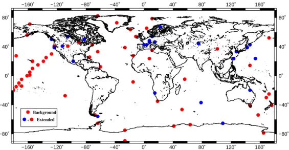
Two networks of surface stations have been used in the dif-ferent inversions of this study: the “background” and the “ex-tended” networks. Red circles in Fig. 1 represent the location of surface stations in the “background” network. The ground” (BG) network is mainly representative of “back-ground” air since most of the surface stations of this network are located far away from the main methane sources. The “extended” (EXT) network is an extension from the back-ground network, where 24 stations are added to the “back-ground” network (blue circles in Fig. 1). These additional stations have been selected for their continental footprint, closer to methane emissions than most of the background sites and therefore providing more direct information on methane emissions. However, being closer to emission areas, and generally located inland, they show more variable mix-ing ratios and are more sensitive to transport errors (Locatelli
et al., 2013). In the following, we use BG and EXT to respec-tively refer to surface measurements in the background and extended configuration of the surface network.
Inversions using these surface observations data sets have been run between 2006 and 2012, but we mainly present re-sults for 2010 to be consistent with the satellite inversions.
2.3.2 One satellite data set: GOSAT
Methane total weighted columns retrieved by GOSAT are also used in our study to constrain methane inversions. Ver-sion 4.0 of the TANSO-FTS XCH4 proxy retrievals
per-formed at the University of Leicester (Parker et al., 2011) are used with associated averaging kernels and a priori profiles. In the “proxy” method, it is considered that the CO2and CH4
spectral absorption bands are close enough to assume that light path perturbations affecting CO2total-column mixing
ratio are similar to those affecting CH4 total-column
mix-ing ratio. Thus, the ratio between the measured CH4 and
CO2vertical mixing ratio is not affected by any perturbations
due to aerosol scattering and clouds. Consequently, the total column of CH4(XCH4) is computed according to XCH4=
[CH4]meas
[CO2]meas×XCO2mod, where [CH4]meas and [CO2]meas are
respectively the CH4 and CO2 measured mixing ratio, and
XCO2modis a model-derived estimate of XCO2coming from
Chevallier et al. (2010)
In the following this data set is referred to as PR-LEI, which stands for “Proxy-Leicester”.
Data from July 2009 to June 2011 are used in the inverse procedure to extract the inferred methane fluxes for the year 2010 with limited time-side effects.
3 Consistency between surface-based and satellite-based inversions
The use of total-column CH4 retrievals from satellite is
fundamental for global inversions as it provides constraints within regions not sampled by surface stations. In particular, satellite data provide information in tropical regions, which are known to largely contribute to the global methane budget and where few surface measurements are available. However, random and systematic errors may be significant in satellite data sets. For example, Houweling et al. (2014) and Berga-maschi et al. (2013) have shown that SCIAMACHY satellite retrievals were usable in methane inversions only if a bias correction algorithm was added. Monteil et al. (2013) also showed inconsistencies between surface and GOSAT inver-sions, which could be explained by space- or time-dependant biases in the GOSAT retrievals. Discrepancies in the model-ing of methane vertical transport in the atmosphere could be another reason for this. Here, using the different versions of the LMDz model, we estimate the inconsistencies between surface-based and satellite-based inversions and we
investi-−160˚ −160˚ −120˚ −120˚ −80˚ −80˚ −40˚ −40˚ 0˚ 0˚ 40˚ 40˚ 80˚ 80˚ 120˚ 120˚ 160˚ 160˚ −80˚ −80˚ −40˚ −40˚ 0˚ 0˚ 40˚ 40˚ 80˚ 80˚ Background Extended +
Figure 1. Location of the surface stations in the “background” (red circles only) and “extended” network (blue and red circles).
90S 60S 30S EQ 30N 60N 90N LATITUDE −40 −20 0 20 40 60 80 100
CH4 simulated − CH4 measured (in pbb)
90S 60S 30S EQ 30N 60N 90N LATITUDE −40 −20 0 20 40 60 80 100
CH4 simulated − CH4 measured (in pbb)
LMDz−TD LMDz−SP
LMDz−NP
LMDz−19
Figure 2. Latitudinal distribution of the bias between simulated methane mixing ratio using an optimized flux distribution coming from a satellite-based inversion and methane mixing ratio measured at different surface stations.
gate the impact of the representation of vertical transport on these inconsistencies.
Four inversions are performed using GOSAT data with-out any bias correction using the three versions of LMDz (LMDz-TD, LMDz-SP, LMDz-NP as described in Sect. 2.2) and the former 19-layer model version (LMDz-19) related to LMDz-TD (Chevallier et al., 2005). The optimized atmo-sphere is then sampled at surface stations and compared to surface observations for the four different versions of the LMDz model (Fig. 2). Methane surface mixing ratios simu-lated from optimized fluxes using GOSAT retrievals do not fit methane mixing ratios directly measured at surface stations (Fig. 2). The different 39-layer versions of the LMDz model show a bias of about +40 ppb, with a small latitudinal depen-dency. This means that, at the surface, the optimized atmo-spheric methane concentrations seen by GOSAT are on aver-age 40 ppb higher than the observed concentrations. Such a
bias can be due to satellite retrievals and/or transport model errors. For comparison, Monteil et al. (2013) found lower but still significant global mean biases of +6.9 and +16.9 ppb in two different GOSAT inversions. Little information is given on the latitudinal distribution of these biases, even though they also seem slightly larger in the Southern Hemisphere than in our study. After analyzing the scaling of the opti-mized initial condition, we found that around 15–20 ppb of the 40 ppb is explained by an increase in the initial condition, the rest being explained by an increase in the CH4emissions.
The similarity of biases derived by LMDz-TD, LMDz-SP and LMDz-NP (Fig. 2) highly suggests that sub-grid-scale parameterizations of vertical transport only play a minor role in inconsistencies between surface and simulated (based on satellite retrievals constraints) methane mixing ratio. Monteil et al. (2013) found similar results performing different sensi-tivity tests to explain inconsistencies between surface-based and satellite-based inversions. As a result, we can conclude that parameterizations of deep convection and diffusion are likely not the cause of these inconsistencies.
Interestingly, we find a very different result with the 19-layer version of LMDz (LMDz-19). Indeed, LMDz-19 de-rives a smaller bias (up to +15 ppb in the high latitudes of the Southern Hemisphere decreasing to down to −10 ppb in the Northern Hemisphere). 19 differs from LMDz-TD only by a coarser vertical resolution. Therefore, a higher vertical resolution seems to degrade the bias of GOSAT in-versions, despite the improvement in the large-scale trans-port shown in Locatelli et al. (2015) for this new version of LMDz.
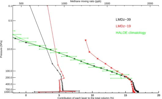
In order to understand this large difference between the two vertical resolutions of the LMDz model, we compare the simulated vertical profiles of methane mixing ratios us-ing LMDz-TD with 19 (LMDz-19) and 39 (LMDz-39) ver-tical levels (Fig. 3). Both simulated profiles use the
corre-0 5 10 15 20
0 5 10 15 20
Contribution of each layer to the total column (%)
500 1000 Methane mixing ratio (ppb) 1500 2000
0.1 0.5 10.0 100.0 200.0 400.0 700.0 1000.0 Pressure (hPa) LMDz−39 LMDz−19 HALOE climatology .
Figure 3. Vertical profiles of methane mixing ratio in ppb (lines with stars) for LMDz-39 (red) and LMDz-19 (black) and compared with HALOE climatology (green). These profiles have been averaged between 60◦N and 60◦S for 2010. Only the contribution (in percent) of each layer of the satellite retrievals to the total column (lines with crosses) is also shown for the two versions of the model. The computation of the model contributions to the total column does not account for the averaging kernel of the satellite retrievals
sponding optimized methane fluxes derived by inversions using the same atmospheric constraints (GOSAT PR-LEI). Figure 3 shows that the CH4profile is very sensitive to the
vertical resolution. The largest differences are found in the stratosphere: LMDz-19 simulates much higher stratospheric methane mixing ratios compared to LMDz-39. However, and consistent with mass balance, LMDz-19 tropospheric mix-ing ratios are smaller than LMDz-39. As found in Locatelli et al. (2015), the two versions of the model have very differ-ent abilities to reproduce stratosphere–troposphere exchange (STE). STE is particularly fast in LMDz-19 compared to LMDz-39, due to a coarser resolution inducing more verti-cal diffusion. This induces stronger methane mixing ratio in the stratosphere in 19. One could think that LMDz-19 simulates a more consistent methane vertical distribution than LMDz-39 as biases in Fig. 2 are smaller for LMDz-19 than for LMDz-39. However, we have compared the mod-eled methane mixing ratio vertical gradients with the clima-tology from the HALOE instrument (Grooß and Russel III, 2005), and we have found extremely similar gradients be-tween LMDz-39 and HALOE data. Indeed, the methane gra-dient between 200 and 3 hPa is 2.2, 5.5 and 5.3 ppb hPa−1for LMDz-19, LMDz-39 and HALOE, respectively. As a result, we find that the relative contribution of each vertical layer to the total column is very different in 39 and LMDz-19 (lines with cross markers in Fig. 3). Stratospheric (tro-pospheric) layers in LMDz-39 contribute much less (more) than in LMDz-19. Consequently, the inverse system derives lower methane fluxes with LMDz-19 to simulate a lower tro-pospheric methane mixing ratio, compensating for the
over-contribution of the stratospheric methane mixing ratio to the total column. The relatively small bias found in the valida-tion of LMDz-19 satellite-based fluxes by surface measure-ments is unfortunately due to an inadequate representation of the troposphere–stratosphere methane mixing ratio gradi-ent. LMDz-39 derives a stronger bias between simulated and surface measurements, but it can be assert that this bias is not due to errors in the modeling of the troposphere–stratosphere gradient, which is improved compared to LMDZ-19. One way to sort out this issue would be to compare to another model such as TM5 model (with 25 vertical levels), which was found to simulate a slower STE than LMDz-19 in Pa-tra et al. (2011) and infers a global mean bias of +6.9 and
+16.9 ppb depending on the GOSAT data set version. Overall, to determine the reason for such biases in satellite inversions still needs more attention on the model side, but most probably also on the data side.
To overcome these model–data inconsistencies, satellite-based inversions are performed in two steps. Firstly, we run inversions using GOSAT data without adding any bias corrections. Secondly, we remove the latitudinal bias found when we compute the difference of the concentrations sim-ulated at each surface stations using the optimized methane fluxes coming from the first inversion with the surface ob-servations considered unbiased. One could argue that the constant part of the bias (∼ 40 ppb) could be absorbed by the initial conditions. This is indeed partly the case for 15– 20 ppb. But the remaining bias translates into additional sur-face emissions, which justifies removing the bias and per-forming a second inversion.
Background Extended PR−LEI 525 530 535 540 545 Inverted CH 4
fluxes in Tg per year
Physics using the Tiedtke scheme (TD) Standard Physics (SP)
New Physics (NP)
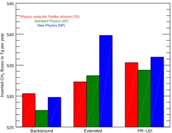
Figure 4. Methane flux estimates (in Tg CH4year−1) for 2010 at the global scale for each inversion (surface inversions using the background and the extended networks, and inversions using proxy products provided by the University of Leicester relative to GOSAT). Inversions using LMDz-TD, LMDz-SP and LMDz-NP as CTM are plotted in red, green and blue, respectively.
In the following, in addition to surface-based inversions, we focus on and present only results associated with these two-step satellite-based inversions.
4 Impact of physical parameterizations on global methane fluxes
Figure 4 displays the sensitivity of the global methane budget to physical parameterizations by showing the global methane estimates from nine inversions using the three different ver-sions of the model (Sect. 2.2) and the three different data sets (Sect. 2.3). Using the BG, EXT, and PR-LEI data sets to constrain methane inversions, we find that the spread (maximum − minimum) in derived methane emissions due to changes in physical parameterizations is respectively 2.7, 7.5, and 2.1 Tg CH4 in 2010. This represents respectively
0.5, 1.4 and 0.4 % of methane global emissions. However, these spreads are lower than when considering changes in atmospheric observations: using TD, SP and NP model ver-sions with the different data sets, we find spreads of 5.0, 6.7 and 10.3 Tg CH4. Therefore, the choice of atmospheric
ob-servations gives more spread in the results than changing model parameterizations, at least in our case. This is un-derstandable, as changing the physical parameterization only accounts for part of the total transport uncertainty. Indeed, the parameterization-based spreads of 2.1 to 7.5 Tg CH4are
much lower than the 27 Tg CH4year−1found in the
pseudo-experiment of Locatelli et al. (2013), which was assumed as an estimate for “total” transport model errors. “Total” here refers to all the possible causes of transport errors. The use of different physical parameterizations within the same CTM
integrated in the same inverse system has a significant impact on global methane emissions, although logically smaller than using different CTMs as done in Locatelli et al. (2013). In-deed, here we only test a few parameterizations of the ver-tical transport in one model. Transport models can also dif-fer in their horizontal resolution and horizontal advection, in their meteorological forcings and the way they constrain atmospheric transport, and in the coupling between their dif-ferent characteristics.
The largest spread (7.5 Tg CH4) for one given data set
is found for the EXT inversions. This is especially due to the EXT-NP inversion, which estimates global methane emissions of 539.8 Tg CH4 in 2010 compared to 532.3 and
533.3 Tg CH4for EXT-TD and EXT-SP, respectively. In
par-ticular, this large estimation is due to a specific region: China. The impact of the parameterizations on the methane flux es-timates for China is further discussed in Sect. 5.
We find that, at the global scale, the spread in GOSAT in-versions (2.1 Tg CH4) is lower than both BG (2.7 Tg CH4)
and EXT (7.5 Tg CH4) surface-based inversions. First,
sub-grid-scale parameterizations in CTMs mainly impact the modeling of vertical transport. An inaccurate representation of methane vertical distribution has larger impacts on simu-lated mixing ratios at the surface than on the simusimu-lated total column. Indeed, a simulation of surface methane mixing ra-tios, which takes place at a specific level of the atmosphere, could miss or underestimate a methane plume if, for exam-ple, methane is transported too quickly into the upper atmo-sphere. However, the simulated total column would not miss this methane plume since it would stay in the atmospheric column, even if the methane plume is simulated at a wrong level. Secondly, surface sources induce weaker signatures in the total-column amounts than in surface concentrations (Rayner and O’Brien, 2001), which could result in a smaller sensitivity of the inverse system to the total column than to surface measurements.
Discrepancies in global methane estimates derived by in-verse modeling are usually largely explained by large-scale characteristics of the modeling of interhemispheric (IH) ex-changes. For example, the overestimation of the north–south gradient in methane mixing ratios in the a priori simulations of the TM5 model have been assumed to be caused by too slow IH exchanges in TM5 (Houweling et al., 1999; Berga-maschi et al., 2009; Monteil et al., 2013). Furthermore, in Pa-tra et al. (2011), LMDz-TD (using a coarser horizontal and vertical resolutions than the version of LMDz-TD used here) is in the range of CTMs simulating a too fast IH exchange, which has been shown to induce a positive (negative) bias in methane emissions in the Northern (Southern) Hemisphere (Locatelli et al., 2013) after inversion.
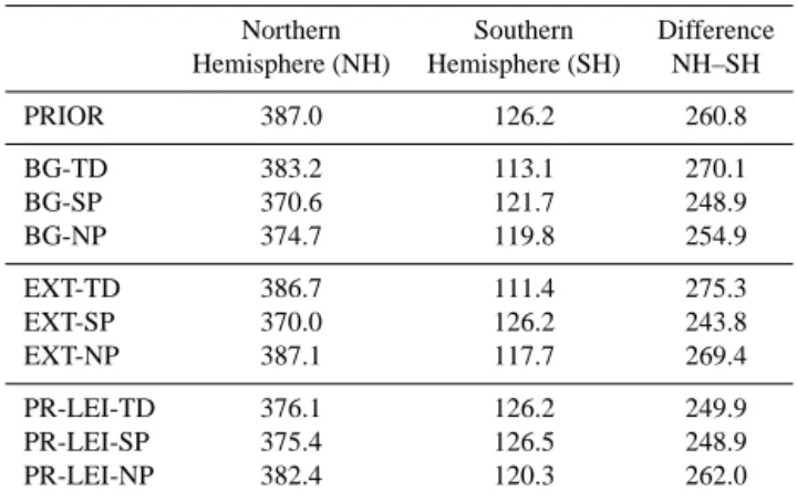
In order to investigate the representation of IH exchange in our inversions, we present in Table 1 the methane estimates in the Northern and the Southern Hemispheres, as well as the IH methane emission gradient for the common year (2010) of the different inversions. Whatever the constraints used in our
Table 1. Annual hemispheric methane fluxes (Tg CH4year−1) for
the common year of simulation (2010).
Northern Southern Difference
Hemisphere (NH) Hemisphere (SH) NH–SH PRIOR 387.0 126.2 260.8 BG-TD 383.2 113.1 270.1 BG-SP 370.6 121.7 248.9 BG-NP 374.7 119.8 254.9 EXT-TD 386.7 111.4 275.3 EXT-SP 370.0 126.2 243.8 EXT-NP 387.1 117.7 269.4 PR-LEI-TD 376.1 126.2 249.9 PR-LEI-SP 375.4 126.5 248.9 PR-LEI-NP 382.4 120.3 262.0
inversions, the hemispheric differences simulated by LMDz-TD are larger compared to those simulated by LMDz-SP. In-deed, BG, EXT, and PR inversions using LMDz-TD derive hemispheric differences of 21.2, 31.5 and 1.0 Tg CH4higher,
respectively, than in inversions using LMDz-SP. These re-sults confirm the conclusion of Locatelli et al. (2015), who showed that LMDz-SP simulates IH exchange slower than LMDz-TD based on an analysis of SF6simulations. Indeed,
LMDz-SP simulating slower IH exchange finds, on aver-age, higher (smaller) methane mixing ratios in the North-ern (SouthNorth-ern) Hemisphere than in LMDz-TD. In response, the inverse system using LMDz-SP derives smaller (higher) methane emissions in the Northern (Southern) Hemisphere to fit the observed mixing ratio. This leads to a smaller hemi-spheric difference in methane emissions compared to what the inverse system derives when it uses LMDz-TD.
Concerning LMDz-NP, results are slightly different. In surface inversions, the hemispheric differences simulated by NP are also smaller than those simulated by LMDz-TD, even if the difference is smaller between LMDz-NP and LMDz-TD than between LMDz-SP and LMDz-TD. How-ever, these results are in agreement with the study of Locatelli et al. (2015), which shows that the thermal plume model im-plemented in LMDz-NP was responsible for a faster IH ex-change in LMDz-NP than in LMDz-SP. Thus, it is not sur-prising to simulate a hemispheric difference of 6.0 Tg CH4
(BG inversions) and 25.6 Tg CH4(EXT inversions) higher in
LMDz-NP than in LMDz-SP. Moreover, the larger difference in EXT compared to BG inversions can be explained by the higher number of stations located closer to methane sources, where the thermal plume model strongly affects the bound-ary layer mixing (Locatelli et al., 2015).
However, the higher hemispheric difference simulated by PR-LEI-NP was not expected from the study of Locatelli et al. (2015). Indeed, PR-LEI-NP simulates a hemispheric difference of 262.0 Tg CH4, which is surprisingly higher than
PR-LEI-TD (249.9 Tg CH4). Large methane emissions are
derived in tropical regions for the year 2010. These re-gions are across the Equator and experience important ver-tical mixing during the year (e.g., monsoon in India). There-fore, they are sensitive to the parameterization of this trans-port. A small but incorrect repartition of emissions between the Northern and Southern Hemisphere can strongly af-fect the hemispheric difference computed here. Moreover, satellite inversions generally derive stronger methane emis-sions in the tropics than surface-based inveremis-sions (Bergam-aschi et al., 2013; Monteil et al., 2013; Houweling et al., 2014). For example, Houweling et al. (2014) found a shift in the emissions from the extra-tropics to the tropics of 50 ± 25 Tg CH4year−1. Thus, one can expect that the
hemi-spheric difference can be changed in satellite-based inver-sions because emisinver-sions can easily be attributed to the South-ern or NorthSouth-ern Hemisphere. However, surface inversions do not have enough constraints to derive accurate tropical emissions which are expected to be high due to strong wet-lands and biomass burning methane emissions. The “miss-ing” amount of methane emissions in tropical regions de-rived by surface inversions are generally shifted to the extra-tropics, which lead to less ambiguous definition of the inter-hemispheric gradient since emissions are clearly attributed to one of the two hemispheres. Moreover, we expect that PR-LEI-NP would simulate a smaller hemispheric difference for a year without such large emissions in the tropics (Houwel-ing et al., 2014).
Overall and across the different data sets assimilated, the largest spread in methane global emission estimations due to parameterization errors reaches 7.5 Tg CH4year−1,
repre-senting 1 % of the total global of methane emissions. The choice of the deep convection scheme has a significant im-pact on the relative distribution of methane emissions be-tween extra-tropical and tropical regions because deep con-vection strongly impacts large-scale atmospheric transport. Versions of LMDz using the deep convection of Emanuel (1991), like LMDz-SP and LMDz-NP, produce a smaller interhemispheric gradient in methane emissions, improving one of the PYVAR inverse system’s flaws identified in Patra et al. (2011) and Locatelli et al. (2013). Among data sets, the impact of parameterization uncertainties on methane emis-sion estimations is smaller when using satellite total-column data compared to surface observations, suggesting that errors related to the modeling of vertical transport have less impact on estimations when considering total-column data.
5 Impact of physical parameterizations on regional methane flux estimates
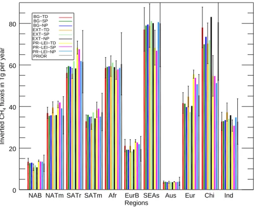
Figure 5 gives a representation of methane flux estimations derived by the nine inversions for 11 continental regions in 2010. Estimations using TD (SP and LMDz-NP) are plotted with different colors (see figure’s legend). The prior estimates for each region are plotted in grey with
NAB NATm SATr SATm Afr EurB SEAs Aus Eur Chi Ind Regions 0 20 40 60 80 Inverted CH 4
fluxes in Tg per year
PRIOR PR−LEI−TD PR−LEI−SP PR−LEI−NP EXT−TD EXT−SP EXT−NP BG−TD BG−SP BG−NP
Figure 5. Estimations of methane fluxes (in Tg CH4year−1) for 11 regions in three versions of the model (LMDz-TD, LMDz-SP and
LMDz-NP) and based on three different observation constraints (BG, EXT and PR-LEI). Prior error bars are overplotted on grey bars, which represent the prior estimations. Posterior error bars are plotted for LMDz-TD inversions only, and they have been estimated based on the work of Cressot et al. (2014). See Sect. 2.1 for more information on the analysis of posterior uncertainties. NAB: North America boreal; NATm: North America temperate; SATr: South America tropical; SATm: South America temperate; Afr: Africa; EurB: Eurasia boreal; SEAs: Southeast Asia; Aus: Australia; Eur: Europe; Chi: China; Ind: India
the associated prior error bars. Posterior error bars are plotted for LMDz-TD inversions only, based on the posterior (resid-ual) errors computed by Cressot et al. (2014) with the same setup and same model (see Sect. 2.1). Comparing emission estimates derived by the different inversions allows us to quantify the impact of sub-grid-scale parameterizations on regional inverted estimates (Sect. 5.1) and to assess its sig-nificance compared to total model errors, to residual errors returned by the inversion, and to the choice of observation data set (Sect. 5.2).
5.1 Quantification of the impact of physical parameterizations on regional methane flux estimates
5.1.1 Surface-based inversions (BG and EXT data sets)
In the BG configuration of surface-based inversions (the first three bars for each region), larger differences are found be-tween inversions using different deep convection schemes than between inversions using different parameterizations of boundary layer mixing. In tropical regions, where deep convection is predominant, like in South America tropical, Southeast Asia or India, it is expected that SP and
BG-NP, which both use the deep convection scheme of Emanuel (1991), derive similar estimates, while BG-TD, which uses the deep convection scheme of Tiedtke (1989), derives slightly different estimations. For example, SP and BG-NP derive estimates of 79.0 and 79.2 Tg CH4year−1,
respec-tively, in Southeast Asia, compared to 76.5 Tg CH4year−1
for BG-TD. However, these changes remain small compared to the residual uncertainties (plotted for LMDz-TD inver-sions in Fig. 5). For extra-tropical regions, where deep con-vection is less directly predominant, like in North Amer-ica temperate, Europe or China, the representation of inter-hemispheric exchange can have large impacts on regional estimates. Indeed, BG inversions are mainly constrained by remote stations (see Sect. 2.3.1), where simulated con-centrations are largely impacted by the representation of large-scale transport (like interhemispheric exchange). How-ever, as mentioned in Sect. 4, the deep convection scheme of Emanuel (1991) has improved the representation of in-terhemispheric exchange in LMDz. Thus, LMDz-SP and LMDz-NP both using the Emanuel (1991) scheme derive similar estimates in regions like North American temperate, Europe or China. Flux estimations for boreal regions (like North America boreal and Eurasia boreal) are also strongly
dependent on the modeling of large-scale atmospheric trans-port since they are far from the main sources of methane. Thus LMDz-SP and LMDz-NP logically derive similar esti-mates in these two boreal regions.
When the extended data set (EXT inversions) is com-bined with the thermal plume model and the Yamada (1983) scheme, LMDz-NP appears to have large impacts. Indeed, this scheme plays a key role in the mixing in the boundary layer and can produce large differences in methane mixing ratio simulated for stations located close to high methane sources as in the EXT network. Thus, large impacts are found in China (five stations have been added close to China in the EXT network), where EXT-NP derives emissions of 74.7 Tg CH4year−1, significantly higher compared to 68.2
and 67.2 Tg CH4year−1 for EXT-SP and EXT-TD,
respec-tively. tropical regions (like in South America tropical) are also affected by the thermal plume model, even if the rea-sons are less obvious than in China, although the thermals play an important role at the base of deep convection lay-ers (Locatelli et al., 2015). However, there are still very few stations constraining tropical emissions in the EXT network.
5.1.2 GOSAT-based inversions (PR-LEI data sets)
However, in PR-LEI inversions, GOSAT data bring strong constraints in tropical regions, where methane sources are supposed to be large. Thus, it is not surprising to see large impacts on tropical region estimates in satellite-based in-versions due to the implementation of the thermal plume model (see the rightmost three bar plots for each re-gion in Fig. 5). Indeed, PR-LEI-TD and PR-LEI-SP derive methane emissions of 68.3 and 67.0 Tg CH4year−1in
South-east Asia, while PR-LEI-NP derives methane emissions of 80.7 Tg CH4year−1in the same region, out of the uncertainty
bounds given for PR-LEI-TD inversion. In South America, PR-LEI-TD and PR-LEI-SP derive larger methane emissions (68.4 and 67.7 Tg CH4year−1) compared to PR-LEI-NP,
which derives methane emissions of 62.0 Tg CH4year−1.
As a consequence, satellite-based inversions derive different spatial distribution in methane emissions between the differ-ent tropical regions (compared to surface-based inversions), although their total methane emissions in the tropics remain close.
5.1.3 Quantification for all regions
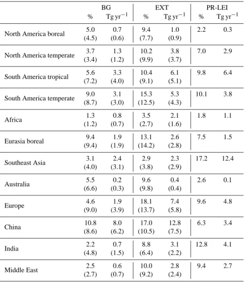
More quantitatively, Table 2 summarizes the spread (differ-ence between the maximum and the minimum of methane emission estimations) in BG, EXT and PR-LEI inversions due to changes in physical parameterizations. The spread is expressed in percent and in Tg CH4year−1. The numbers are
relative to the common year of inversions, which is 2010. However, average spreads between 2007 and 2011 are also shown for BG and EXT inversions (inside the parentheses in Table 2) since surface-based inversions have been run
for several years (2006–2012). First, one can notice that the spreads (in percent) at regional scales caused by changes in sub-grid-scale parameterizations appear larger compared to what was found at the global scale (see Sect. 4). Indeed, at regional scales, spreads range from 1 to 11 % (0.2 to 8.0 Tg CH4year−1), 3 to 18 % (0.4 to 12.8 Tg CH4year−1)
and 2 to 17 % (0.1 to 12.4 Tg CH4year−1) for BG, EXT
and PR-LEI inversions, respectively. Across the networks, the largest spreads (in Tg CH4year−1) are found in China,
Southeast Asia, Europe, South America tropical and South America temperate. Furthermore, spreads in surface-based inversions are larger in EXT compared to BG configuration of the surface network, similar to what we found at the global scale. Indeed, constraints added in EXT inversions are lo-cated closer to large methane mixing ratio gradients, which makes EXT inversions more sensitive to the modeling of the boundary layer mixing. Yet, skills of the different LMDz versions (LMDz-TD, LMDz-SP and LMDz-NP) to simulate PBL mixing can be highly different (Locatelli et al., 2015). Thus, the different configurations of the inverse system in-duce larger spreads in EXT compared to BG inversions. On average, the mean regional spread is 5, 11 and 8 % for BG, EXT and PR-LEI inversions, respectively. This gives a mean error of 8 % at regional scales considering the three types of inversions.
5.2 Significance of the impact of physical parameterizations at regional scales
A question arising from the previous section is the signifi-cance of the spread due to physical parameterizations com-pared to others errors: total transport error, residual error from the inversion and spread in methane emissions due to the choice of the observing network. Thus, we compare here the impact of physical parameterization uncertainties on methane inversions with these three sources of errors.
5.2.1 Physical parameterizations versus total transport error
Similar to results found for the global scale, spreads at regional scales when using different parameterizations in LMDz are smaller than spreads between inversions using different atmospheric transport models as in Locatelli et al. (2013). Indeed, in Locatelli et al. (2013), spreads between in-versions using different CTMs range from 23 % for Europe to 48 % for South America, with an average of 33 %. Here, we found that the mean error in methane estimates due to parameterization errors is 8 % at regional scales (Sect. 5.1). Consequently, if one assumes that the spread given in Lo-catelli et al. (2013) is representative of the total error due to the modeling of transport, errors related to physical param-eterizations explain, on average 24 % (corresponding to the ratio of 8/33) of the total transport model errors, but it can reach more than 50 % in some specific regions. Therefore,
Table 2. Spreads of regional methane flux (maximum − minimum of CH4emissions) in BG, EXT and PR-LEI inversions due to changes in physical parameterizations. The spread is expressed in percent and in Tg CH4year−1. The numbers are relative to the common year
of inversions, which is 2010. However, average spreads between 2007 and 2011 are also shown for BG and EXT inversions (inside the parentheses) since surface-based inversions have been run for several years.
BG EXT PR-LEI
% Tg yr−1 % Tg yr−1 % Tg yr−1
North America boreal 5.0 0.7 9.4 1.0 2.2 0.3
(4.5) (0.6) (7.7) (0.9)
North America temperate 3.7 1.3 10.2 3.8 7.0 2.9
(3.4) (1.2) (9.9) (3.7)
South America tropical 5.6 3.3 10.4 6.1 9.8 6.4
(7.2) (4.0) (9.1) (5.1)
South America temperate 9.0 3.1 15.3 5.3 10.1 3.8 (8.7) (3.0) (12.5) (4.3) Africa 1.3 0.8 3.5 2.1 1.8 1.1 (1.2) (0.7) (2.7) (1.6) Eurasia boreal 9.4 1.9 13.1 2.6 7.5 1.5 (9.4) (1.9) (14.2) (2.8) Southeast Asia 3.1 2.4 2.9 2.3 17.2 12.4 (4.0) (3.1) (3.8) (2.9) Australia 5.5 0.2 9.6 0.4 2.6 0.1 (6.6) (0.3) (9.8) (0.4) Europe 4.6 1.9 18.1 7.4 9.6 4.8 (9.0) (3.9) (13.7) (5.8) China 10.8 8.0 17.0 12.8 6.3 3.4 (8.6) (6.2) (10.5) (7.5) India 2.2 0.7 8.8 3.1 12.8 4.1 (4.8) (1.5) (6.4) (2.2) Middle East 2.5 0.6 10.0 2.8 9.4 2.7 (2.7) (0.7) (9.2) (2.4)
the different parameterizations used within LMDz span rel-atively more of the transport error at regional scales than at the global scale.
5.2.2 Physical parameterizations versus residual errors
One can compare the spreads in methane emission estimates due to parameterization uncertainties in different regions in Fig. 5 to the amplitudes of posterior (residual) uncertain-ties estimated by Cressot et al. (2014). A spread in methane inversion estimates that is larger than the amplitude of the posterior uncertainties is found for three regions only: South America tropical, Europe and China. Consequently, one can interpret that the impact of parameterization uncertainties in these three regions is meaningful. An improvement of the representation of sub-grid processes could significantly in-crease the confidence in methane emission estimates in these regions. In the other regions, the spreads in inverted estimates
are found to be similar to (Eurasia boreal, North America temperate, South America temperate) or smaller than (Africa and India) the amplitudes of posterior uncertainties, indicat-ing that changes due to the use of different parameterizations are less meaningful for these regions.
5.2.3 Physical parameterizations versus the choice of observation networks
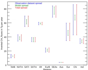
As already mentioned regarding the global scale, the spread in methane inverted regional estimates is in general smaller when one considers inversions constrained by the same ob-servation data set (Fig. 6). Comparing the spread in inver-sions using a same observation data set but different verinver-sions of LMDz (green bar plots in Fig. 6) with inversions using the same version of LMDz but different observation data sets (blue bar plots) shows that the choice of observation data set has a larger impact on inverted regional estimates. Spreads
NAB NATm SATr SATm Afr EurB SEAs Aus Eur Chi Ind Regions 0 20 40 60 80 Inverted CH 4
fluxes in Tg per year
Observation dataset spread Model spread
Total spread
Figure 6. Spreads (maximum − minimum) in regional methane es-timates (in Tg CH4year−1) due to the choice of the observation data
set (blue error bars) and due to the choice of the model version (green error bars). The total spreads in the nine inversions run in this work are plotted in red.
in inversions based on different versions of LMDz are sim-ilar (or slightly smaller) to spreads in inversions based on different observation data sets in South America temperate, Africa, Eurasia boreal, India and Australia. But, in all the others regions, the spreads in inversions based on different observation data sets are much larger. This is especially ob-vious in Europe, China and South America tropical. Indeed, information provided by the different data sets is different but can also be differently interpreted by the different versions of LMDz. A good example of this assessment is found in tropi-cal regions for inversions constrained by the PR-LEI data set. The inverse system based on LMDz-NP derives a very dif-ferent spatial distribution: larger emissions in Southeast Asia but lower emissions in South America tropical compared to inversions based on LMDz-TD and LMDz-SP.
Overall, we find that, if the choice of the observation data set used to constrain the inversion generally remains a larger source of uncertainty than the change in physical parameteri-zations for one given data set, both can generate significantly different spatial distributions of methane emissions, espe-cially within the tropics and for Europe and China. For ex-ample, the partition of methane emissions within the tropics can shift from Southeast Asia to South America and methane emission estimates derived by BG and PR-LEI inversions differ by 15 and 22 Tg CH4year−1in Europe and China,
re-spectively (Fig. 5).
6 Conclusions
This study presents the sensitivity of the recent methane bud-get estimated by the PYVAR inversion system to different
LMDz sub-grid-scale physical parameterizations for verti-cal transport, combined with different observation data sets. Three versions of LMDz (TD, SP and LMDz-NP) have been used within the PYVAR system to simulate at-mospheric transport of methane emitted at the surface. Three methane observation data sets (two surface data sets and one GOSAT data set) have been assimilated to constrain these different atmospheric inversions. Finally, the comparison be-tween these nine inversions quantifies the impact of LMDz sub-grid-scale parameterizations on methane inverted esti-mates.
Satellite-based inversions generate atmospheric mixing ra-tios, which are inconsistent with surface observations when no bias correction is applied. These inconsistencies are not related to the physical parameterizations of the vertical trans-port for LMDz. The relative agreement between methane concentrations simulated by the former version of LMDz and GOSAT data masks a poor representation of the methane gra-dient at the tropopause in the former version of the LMDz model. However, our results based on different new ver-sions of LMDz, properly reproducing the vertical gradient of methane in the upper troposphere/lower stratosphere, sug-gest a large bias in the GOSAT data (∼ 40 ppb), with a small latitudinal dependency. This bias is corrected to analyze and compare the different inversions performed.
At the global scale, we find that the spread due to phys-ical parameterization uncertainties is 0.5, 1.4 and 0.4 % of global methane emissions. Moreover, the analysis of the north–south gradient in inferred emissions confirms that the Emanuel (1991) deep convection scheme improves the repre-sentation of IH exchange, as already mentioned in Locatelli et al. (2015).
At regional scales, the spreads due to physical parameteri-zation are larger than at the global scale (5–11 %) but remain generally lower than the spread due to the choice of observa-tion data set and always lower (24 % on average) than the to-tal uncertainty due to the modeling of atmospheric transport as estimated by Locatelli et al. (2013). Comparison of these spreads to the residual regional inversion uncertainties given in Cressot et al. (2014) indicates that they are significant for a few key regions of the methane cycle: South America, China and Europe. Indeed, changing the parameterizations can lead to significantly different spatial partitions of methane emis-sions for (or between) these regions. One important addi-tional result is that the thermal plume model combined with the vertical diffusion scheme of Yamada (1983) implemented in LMDz-NP largely impact regional estimations, especially when considering atmospheric constraints located close to high methane sources (like in tropical regions for satellite-based inversions).
After the quantification of transport model errors in global and regional methane flux estimates based on a TransCom intercomparison (Locatelli et al., 2013) and the evaluation of new parameterizations in LMDz to simulate trace gas con-centrations (Locatelli et al., 2015), this paper goes one step
further in the understanding and the quantification of causes and impacts of model errors in methane inversions. In these different studies, precisions have been given on the degree of confidence in the global and regional methane estimations using inverse modeling relative to transport model errors. At the global scale, the impact of transport model errors (5 % of global methane emissions) and physical parameterizations errors (0.8 %) is acceptable. However, the picture is differ-ent at regional scales, with a possible significant impact of transport errors on the attribution of regional methane emis-sion estimated by inverse modeling. A striking finding of our work is the possibility to change the partition of methane tropical emissions depending on the combination of obser-vation data set and physical parameterizations used, even af-ter correcting probable biases in satellite data sets. Our work provides elements to understand why the different inversions recently published lack regional consistency with each other in their attribution of the renewed increase in atmospheric methane since 2007. Our results indicate a need for more work to be carried out to improve transport models in order to reduce transport errors. A way to achieve this is, for one, to strengthen collaborations between experts in atmospheric dynamics and experts in tracer transport and, for another, to develop measurement campaigns and use specific tracers in order to better evaluate transport models on the other hand. Finally, inconsistencies between surface-based and satellite-based inversions need to receive more attention in the future.
Acknowledgements. This work is supported by the DGA (Direction Générale de l’Armement) and CEA (Centre à l’Energie Atomique et aux Energies Alternatives).
We would like to thank Vanessa Sherlock, Yi Yin, Frédéric Hour-din and Catherine Rio for fruitful discussions. We would like also thank Sébastien Leonard for his IT support.
The authors wish to thank R. Parker and H. Boesch (EOS, Uni-versity of Leicester) for providing the GOSAT Proxy XCH4 data set. This product was developed partly with funding from the ESA GHG-CCI project and the UK National Centre for Earth Observa-tion.
We acknowledge the contributors to the World Data Centre for Greenhouse Gases for providing their data of methane and methyl chloroform atmospheric mole fractions. The authors thank in particular A. J. Gomez-Pelaez (AEMET), R. Prinn (AGAGE), R. Weiss (AGAGE), P. Krummel (CSIRO), D. Worthy (EC), S. Piacentino (ENEA), Y. Fukuyama (JMA), Y. Tohjima (NIES), E. Dlugokencky (NOAA) and K. Uhse (UBA). Moreover, the authors wish to thank the respective funding organizations/institutions for their long-term support of these measurement programs.
Edited by: P. Jöckel
References
Bergamaschi, P., Krol, M., Dentener, F., Vermeulen, A., Meinhardt, F., Graul, R., Ramonet, M., Peters, W., and Dlugokencky, E. J.: Inverse modelling of national and European CH4emissions
us-ing the atmospheric zoom model TM5, Atmos. Chem. Phys., 5, 2431–2460, doi:10.5194/acp-5-2431-2005, 2005.
Bergamaschi, P., Frankenberg, C., Meirink, J. F., Krol, M., Dentener, F., Wagner, T., Platt, U., Kaplan, J. O., Körner, S., Heimann, M., Dlugokencky, E. J., and Goede, A.: Satellite chartography of atmospheric methane from SCIA-MACHY on board ENVISAT: 2. Evaluation based on inverse model simulations, J. Geophys. Res.-Atmos., 122, D02304, doi:10.1029/2006JD007268, 2007.
Bergamaschi, P., Frankenberg, C., Meirink, J. F., Krol, M., Vil-lani, M. G., Houweling, S., Dentener, F., Dlugokencky, E. J., Miller, J. B., Gatti, L. V., Engel, A., and Levin, I.: In-verse modeling of global and regional CH4 emissions using SCIAMACHY satellite retrievals, J. Geophys. Res.-Atmos., 114, D22301, doi:10.1029/2009JD012287, 2009.
Bergamaschi, P., Krol, M., Meirink, J. F., Dentener, F., Segers, A., van Aardenne, J., Monni, S., Vermeulen, A. T., Schmidt, M., Ramonet, M., Yver, C., Meinhardt, F., Nisbet, E. G., Fisher, R. E., O’Doherty, S., and Dlugokencky, E. J.: Inverse modeling of European CH4emissions 2001–2006, J. Geophys. Res., 115,
D22309, doi:10.1029/2010JD014180, 2010.
Bergamaschi, P., Houweling, S., Segers, A., Krol, M., Frankenberg, C., Scheepmaker, R. A., Dlugokencky, E. J., Wofsy, S. C., Kort, E. A., Sweeney, C., Schuck, T., Brenninkmeijer, C., Chen, H., Beck, V., and Gerbig, C.: Atmospheric CH4in the first decade of
the 21st century: Inverse modeling analysis using SCIAMACHY satellite retrievals and NOAA surface measurements, J. Geophys. Res.-Atmos., 118 7350–7369, doi:10.1002/jgrd.50480, 2013. Bousquet, P., Hauglustaine, D. A., Peylin, P., Carouge, C., and
Ciais, P.: Two decades of OH variability as inferred by an in-version of atmospheric transport and chemistry of methyl chlo-roform, Atmos. Chem. Phys., 5, 2635–2656, doi:10.5194/acp-5-2635-2005, 2005.
Bousquet, P., Ciais, P., Miller, J. B., Dlugokencky, E. J., Hauglus-taine, D. A., Prigent, C., Van der Werf, G. R., Peylin, P., Brunke, E.-G., Carouge, C., Langenfelds, R. L., Lathiere, J., Papa, F., Ramonet, M., Schmidt, M., Steele, L. P., Tyler, S. C., and White, J.: Contribution of anthropogenic and natural sources to atmospheric methane variability, Nature, 443, 439– 443, doi:10.1038/nature05132, 2006.
Bousquet, P., Ringeval, B., Pison, I., Dlugokencky, E. J., Brunke, E.-G., Carouge, C., Chevallier, F., Fortems-Cheiney, A., Franken-berg, C., Hauglustaine, D. A., Krummel, P. B., Langenfelds, R. L., Ramonet, M., Schmidt, M., Steele, L. P., Szopa, S., Yver, C., Viovy, N., and Ciais, P.: Source attribution of the changes in atmospheric methane for 2006–2008, Atmos. Chem. Phys., 11, 3689–3700, doi:10.5194/acp-11-3689-2011, 2011.
Chevallier, F.: On the parallelization of atmospheric inversions of CO2 surface fluxes within a variational framework, Geosci. Model Dev., 6, 783–790, doi:10.5194/gmd-6-783-2013, 2013. Chevallier, F., Fisher, M., Peylin, P., Serrar, S., Bousquet, P.,
Bréon, F.-M., Chédin, A., and Ciais, P.: Inferring CO2sources
and sinks from satellite observations: Method and applica-tion to TOVS data, J. Geophys. Res.-Atmos., 110, D24309, doi:10.1029/2005JD006390, 2005.
Chevallier, F., Bréon, F.-M., and Rayner, P. J.: Contribution of the Orbiting Carbon Observatory to the estimation of CO2
sources and sinks: Theoretical study in a variational data as-similation framework, J. Geophys. Res.-Atmos., 112, D09307, doi:10.1029/2006JD007375, 2007.
Chevallier, F., Feng, L., Bösch, H., Palmer, P. I., and Rayner, P. J.: On the impact of transport model errors for the estimation of CO2 surface fluxes from GOSAT observations, Geophys. Res.
Lett., 37, L21803, doi:10.1029/2010GL044652, 2010.
Chevallier, F., Palmer, P. I., Feng, L., Boesch, H., O’Dell, C. W., and Bousquet, P.: Toward robust and consistent re-gional CO2flux estimates from in-situ and spaceborne
measure-ments of atmospheric CO2, Geophys. Res. Lett., 41, 1065–1070,
doi:10.1002/2013GL058772, 2014.
Cressot, C., Chevallier, F., Bousquet, P., Crevoisier, C., Dlugo-kencky, E. J., Fortems-Cheiney, A., Frankenberg, C., Parker, R., Pison, I., Scheepmaker, R. A., Montzka, S. A., Krummel, P. B., Steele, L. P., and Langenfelds, R. L.: On the consistency between global and regional methane emissions inferred from SCIA-MACHY, TANSO-FTS, IASI and surface measurements, Atmos. Chem. Phys., 14, 577–592, doi:10.5194/acp-14-577-2014, 2014. Dee, D. P., Uppala, S. M., Simmons, A. J., Berrisford, P., Poli, P., Kobayashi, S., Andrae, U., Balmaseda, M. A., Balsamo, G., Bauer, P., Bechtold, P., Beljaars, A. C. M., van de Berg, L., Bid-lot, J., Bormann, N., Delsol, C., Dragani, R., Fuentes, M., Geer, A. J., Haimberger, L., Healy, S. B., Hersbach, H., Holm, E. V., Isaksen, L., Kallberg, P., Kohler, M., Matricardi, M., McNally, A. P., Monge-Sanz, B. M., Morcrette, J.-J., Park, B.-K., Peubey, C., de Rosnay, P., Tavolato, C., Thépaut, J.-N., and Vitart, F.: The ERA-Interim reanalysis: configuration and performance of the data assimilation system, Q. J. Roy. Meteorol. Soc., 137, 553– 597, doi:10.1002/qj.828, 2011.
Emanuel K. A. L.: A Scheme for Representing Cumulus Con-vection in Large-Scale Models, J. Atmos. Sci., 48, 2313–2329, doi:10.1175/1520-0469(1991)048<2313:ASFRCC>2.0.CO;2, 1991.
Enting, I. G.: Inverse problems in atmospheric constituent transport, CUP, Cambridge, UK, 2002.
Fortems-Cheiney A., Chevallier, F., Pison, I., Bousquet, P., Szopa, S., Deeter, M. N., and Clerbaux, C.: Ten years of CO emis-sions as seen from Measurements of Pollution in the Tro-posphere (MOPITT), J. Geophys. Res.-Atmos., 116, D05304, doi:10.1029/2010JD014416, 2011.
Frankenberg, C., Meirink, J. F., van Weele, M., Platt, U., and Wagner, T.: Assessing Methane Emissions from Global Space-Borne Observations, Science, 308, 1010–1014, doi:10.1126/science.1106644, 2005.
Frankenberg, C., Bergamaschi, P., Butz, A., Houweling, S., Meirink, J. F., Notholt, J., Petersen, A. K., Schrijver, H., Warneke, T., and Aben, I.: Tropical methane emissions: A re-vised view from SCIAMACHY onboard ENVISAT, Geophys. Res. Lett., 35, L15811, doi:10.1029/2008GL034300, 2008. Geels, C., Gloor, M., Ciais, P., Bousquet, P., Peylin, P., Vermeulen,
A. T., Dargaville, R., Aalto, T., Brandt, J., Christensen, J. H., Frohn, L. M., Haszpra, L., Karstens, U., Rödenbeck, C., Ra-monet, M., Carboni, G., and Santaguida, R.: Comparing at-mospheric transport models for future regional inversions over Europe – Part 1: mapping the atmospheric CO2 signals,
At-mos. Chem. Phys., 7, 3461–3479, doi:10.5194/acp-7-3461-2007, 2007.
Gilbert J.-C. and Lemaréchal, C.: Some numerical experiments with variable-storage quasi-Newton algorithms, Math. Program., 45, 407–435, doi:10.1007/BF01589113, 1989.
Grooß, J.-U. and Russell III, James M.: Technical note: A strato-spheric climatology for O3, H2O, CH4, NOx, HCl and HF
derived from HALOE measurements, Atmos. Chem. Phys., 5, 2797–2807, doi:10.5194/acp-5-2797-2005, 2005.
Hourdin, F. and Armengaud, A.: The Use of Finite-Volume Methods for Atmospheric Advection of Trace Species, Part I: Test of Various Formulations in a General Circulation Model, Mon. Weather Rev., 127, 822–837, doi:10.1175/1520-0493(1999)127<0822:TUOFVM>2.0.CO;2, 1999.
Hourdin, F., Couvreux, F., and Menut, L.: Parameterization of the Dry Convective Boundary Layer Based on a Mass Flux Representation of Thermals, J. Atmos. Sci., 59, 1105–1123, doi:10.1175/1520-0469(2002)059<1105:POTDCB>2.0.CO;2, 2002.
Hourdin, F., Musat, I., Bony, S., Braconnot, P., Codron, F., Dufresne, J.-L., Fairhead, L., Filiberti, M.-A., Friedlingstein, P., Grandpeix, J.-Y., Krinner, G., LeVan, P., Li, Z.-X., and Lott, F.: The LMDZ4 general circulation model: climate performance and sensitivity to parametrized physics with emphasis on tropical convection, Clim. Dynam., 27, 787–813, doi:10.1007/s00382-006-0158-0, 2006.
Hourdin, F., Foujols, M.-A., Codron, F., Guemas, V., Dufresne, J.-L., Bony, S., Denvil, S., Guez, J.-L., Lott, F., Ghattas, J., Braconnot, P., Marti, O., Meurdesoif, Y., and Bopp, L.: Impact of the LMDZ atmospheric grid configuration on the climate and sensitivity of the IPSL-CM5A coupled model, Clim. Dynam., 40, 2167–2192, doi:10.1007/s00382-012-1411-3, 2012a.
Hourdin, F., Grandpeix, J.-Y., Rio, C., Bony, S., Jam, A., Cheruy, F., Rochetin, N., Fairhead, L., Idelkadi, A., Musat, I., Dufresne, J.-L., Lahellec, A., Lefebvre, M.-P., and Roehrig, R.: LMDZ5B: the atmospheric component of the IPSL climate model with revisited parameterizations for clouds and convection, Clim. Dynam., 40, 2193–2222, doi:10.1007/s00382-012-1343-y, 2012b.
Houweling, S., Kaminski, T., Dentener, F., Lelieveld, J., and Heimann, M.: Inverse modeling of methane sources and sinks using the adjoint of a global transport model, J. Geophys. Res., 104, 26137, doi:10.1029/1999JD900428, 1999.
Houweling, S., Dentener, F., and Lelieveld, J.: Simulation of prein-dustrial atmospheric methane to constrain the global source strength of natural wetlands, J. Geophys. Res.-Atmos., 105, 17243–17255, doi:10.1029/2000JD900193, 2000.
Houweling, S., Röckmann, T., Aben, I., Keppler, F., Krol, M., Meirink, J. F., Dlugokencky, E. J., and Frankenberg, C.: Atmo-spheric constraints on global emissions of methane from plants, Geophys. Res. Lett., 33, L15821, doi:10.1029/2006GL026162, 2006.
Houweling, S., Aben, I., Breon, F.-M., Chevallier, F., Deutscher, N., Engelen, R., Gerbig, C., Griffith, D., Hungershoefer, K., Macatangay, R., Marshall, J., Notholt, J., Peters, W., and Serrar, S.: The importance of transport model uncertainties for the esti-mation of CO2sources and sinks using satellite measurements,
Atmos. Chem. Phys., 10, 9981–9992, doi:10.5194/acp-10-9981-2010, 2010.