Optimizing Partition Trees for Multi-Object Segmentation with Shape Prior

(1)

HAL Id: hal-01182776

https://hal.inria.fr/hal-01182776

Submitted on 3 Aug 2015

HAL is a multi-disciplinary open access

archive for the deposit and dissemination of

sci-entific research documents, whether they are

pub-lished or not. The documents may come from

teaching and research institutions in France or

abroad, or from public or private research centers.

L’archive ouverte pluridisciplinaire HAL, est

destinée au dépôt et à la diffusion de documents

scientifiques de niveau recherche, publiés ou non,

émanant des établissements d’enseignement et de

recherche français ou étrangers, des laboratoires

publics ou privés.

Optimizing Partition Trees for Multi-Object

Segmentation with Shape Prior

Emmanuel Maggiori, Yuliya Tarabalka, Guillaume Charpiat

To cite this version:

Emmanuel Maggiori, Yuliya Tarabalka, Guillaume Charpiat. Optimizing Partition Trees for

Multi-Object Segmentation with Shape Prior. 26th British Machine Vision Conference, Sep 2015, Swansea,

United Kingdom. �hal-01182776�

(2)

MAGGIORI ET AL.: OPTIMIZING PARTITION TREES FOR SEGMENTATION

Optimizing Partition Trees for Multi-Object

Segmentation with Shape Prior

Emmanuel Maggiori1 [email protected] Yuliya Tarabalka1 [email protected] Guillaume Charpiat2 [email protected]

1_{Inria Sophia Antipolis Méditerranée}

Titane team

Sophia Antipolis, France

2_{Inria Saclay}

TAO team Orsay, France

Abstract

A partition tree is a hierarchical representation of an image. Once constructed, it can be repeatedly processed to extract information. Multi-object multi-class image segmen-tation with shape priors is one of the tasks that can be efficiently done upon an available tree. The traditional construction approach is a greedy clustering based on color simi-larities. However, not considering higher level cues during the construction phase leads to trees that might not accurately represent the underlying objects in the scene, inducing mistakes in the later segmentation. We propose a method to optimize a tree based both on color distributions and shape priors. It consists in pruning and regrafting tree branches in order to minimize the energy of the best segmentation that can be extracted from the tree. Theoretical guarantees help reducing the search space and make the optimization efficient. Our experiments show that we succeed in incorporating shape information to restructure a tree, which in turn enables to extract from it good quality multi-object seg-mentations with shape priors.

1 Introduction

The multi-object segmentation of images is one of the great challenges in computer vision. It consists in the simultaneous partitioning of an image into regions and in the assignment of labels to each of the segments. It contemplates the existence of many objects of possibly different classes in the same image.

In the last years, hierarchical partitions have been intensively used in different domains. The overall idea is to represent an image as a tree of hierarchical partitions, which is later processed to extract meaningful information. The construction of a high quality hierarchical representation is useful per se, given that it allows to repeatedly explore the data at different scales and for different purposes, at a low computational cost. Visual browsing [21], object localization [29] and depth ordering [19] are some of the activities that can be efficiently done upon an already available hierarchical representation. Binary partition trees (BPTs) [21] are a particularly efficient structure for this purpose. In our context, multi-object segmentations can be extracted from such trees by selecting scales in different branches.

c

2015. The copyright of this document resides with its authors. It may be distributed unchanged freely in print or electronic forms.

(3)

The introduction of shape descriptors into segmentation significantly improves its quality [5]. However, it is difficult to optimize energies that involve shape priors because of their non-local nature [14]. BPTs can be easily augmented to include shape information, but their traditional greedy construction approach does not yield a good utilization of the shape constraints.

In this work we exploit the idea of iteratively optimizing the structure of BPTs to produce better partitions with shape priors. Our contribution is two-fold:

• we propose a framework for multi-class multi-object segmentation with shape priors based on optimized BPTs,

• our technique enhances BPTs so that they can better represent the underlying scenes.

2 Related work

A number of techniques to include shape features in segmentation have been presented. We here deal with discriminative features (e.g. compactness, ellipticity) rather than strict tem-plate matching. In this direction, a number of works have managed to express certain features in submodular energy terms that can be minimized by s-t cuts (star-shape [28], compactness [6,8]), though this is not feasible for any feature. The trust regions framework [10] has been adapted for certain high order priors (volume and shape moments [10], convexity [11]), though it requires a linear approximation of the energy around the current solution, which might not be straightforward for other priors (e.g. rectangularity index). Moreover, these techniques do not contemplate the occurrence of multiple object instances. It is required to isolate every object (with prior knowledge on its location) and segment it individually, otherwise the existence of multiple instances is penalized by the shape prior itself.

Regarding BPTs, recent works have included shape descriptors into the structure [26,29]. However, due to the traditional greedy construction approach, it is very likely that nodes in the BPT will not represent complete significant objects [16, 29]. Enhanced construction functions (e.g., [13,24,29]) can only alleviate the effect. Shape information cannot be used at construction: the ultimate shape of an object in a branch cannot be predicted by a portion of it. As a result, the criteria used at construction and at processing are different (as in [26,29]), which limits the feasibility of the tool as it is to perform segmentation with shape prior.

Possibly the most related work has been done in the area of computational phylogenetics, on the construction of phylogenetic trees [15]. Several traditional optimization algorithms have been applied by performing local transformations on the tree structures to maximize the so-called parsimony [9]. We have incorporated the idea of regrafting tree branches. Our optimization objective is however different, and our context requires to define moves that preserve the parent, child and spatial adjacency relations of BPTs.

3 Segmentation as an optimization problem

Let I = (Ij)16 j6nbe an input image containing n pixels. We suppose we are given a set of

possible object classes, as well as priors for each class. Multi-label segmentation consists in the partitioning of the pixels into a non-overlapping set of regions R = (Ri), together with

(4)

MAGGIORI ET AL.: OPTIMIZING PARTITION TREES FOR SEGMENTATION E(R, L) = EC(I, R, L) + |R|

∑

i=1 ES(Ri, Li), (1)

where EC expresses the color prior (quantifying how much the segmentation fits the image

colors), and ES, the shape prior. We have here assumed equal class occurrence probabilities.

The reader is referred to the supplementary material for a formulation in the general case. For each object class, we suppose we are given training examples, from which the color distribution can be estimated and used as a prior. Given a candidate segmentation (R, L), let us denote by L_{R( j)}the label of the region containing a pixel j. The color prior is:

EC(I, R, L) = n

∑

j=1

− log P(LR( j)|Ij). (2)

One way of obtaining the posterior P(L_{R( j)}|Ij) is to train classifiers based on the samples’

colors, using support vector machines (SVM), and to extend them to output probability esti-mates as usual in classification problems [30].

Similarly, the shape prior term is defined as follows:

ES(Ri, Li) = −|Ri| log P(Li|Si), (3)

|Ri| being the area of region Ri, and P(Li|Si) being the probability of assigning the label Li

to the region Ri, given a vector Siof shape features of that region. Traditional regularization

(such as boundary length [18]) can be incorporated as part of this term. The weight on the area makes the per-pixel contribution of the color prior and the per-region contribution of the shape prior equally important.

We wish to enrich the nodes of BPTs by including shape information of the regions. Given that the optimization of the trees will involve recomputing region descriptors, we must design a pool of features that can be computed efficiently from children nodes. We propose to store the convex hull of the region at every node. When two regions are merged, the convex hull of the new region can be computed by merging the convex hulls of its children. This can be done in linear time in the size of the input polygons by using rotating calipers [25]. Many useful shape descriptors can be derived from the convex hull. Solidity is the ratio between the area of a shape and the area of its convex hull, and is useful to measure the convexity of the object [31]. The minimum area enclosing rectangle (sized w × h) of a region Ris efficiently computed from the convex hull [25], and other descriptors are derived after it, such as rectangularity index (|R|/(h · w)) and elongatedness (w/h) [31]. In a balanced tree, which is enforced by our construction function, convex hulls incur in an O(n log(n)) increase of the storage required and their computation does not increase the complexity of tree con-struction (proofs in suppl. material). Another useful shape descriptor is compactness [17], related to the resemblance to a circle. It is typically defined as δ R2/(4π|R|), where δ R is the perimeter of R. However, this formulation imposes difficulties in a discrete environment [17] due to the fact that the error in the estimation of δ R does not converge. In [24] the authors proved the robustness of computing compactness as |R|2/(2πIg), Igbeing the moment of

in-ertia of the shape with respect to its centroid. Given that the centroid and moment of inin-ertia of a region can be computed in constant time from the children, we propose this method to measure compactness in BPTs.

Let us suppose a probability density function p(s|L) is available for every feature and class. These densities can be obtained by smoothing histograms of training samples [23]. Let us call S = s1, ..., sma vector of shape features. Assuming features’ conditional

(5)

(a) BPT and segmentation by pruning. (b) Faulty BPT, an object (bcde)

not represented in a single node.

Figure 1: Binary partition trees.

P(L|S) ∝ m

∏

k=1 P(L|sk) = m

∏

k=1 p(sk|L) ∑ Lj∈L p(s_k|Lj) . (4)

Combining Eq. (1), (2) and (3), the energy criterion to minimize is formulated as:

E(R, L) = − |R|

∑

i=1 j∈R

∑

i log P(Li|Ij) + |Ri| log P(Li|Si) ! . (5)

4 Building and processing a partition tree

In this section we show how to build a first candidate solution to the problem (5), in a bottom-up manner, before presenting our optimization approach (Section5).

4.1 Building a partition tree

Our initialization involves the construction of a BPT, without any introduction of shape infor-mation. BPTs are built by using a bottom-up region merging approach [2]. At each iteration, the two most similar regions are merged into a bigger one and a node representing the new region is added to the BPT, connected to its two corresponding children (see Fig.1a). The final tree contains exactly 2n − 1 nodes, where the root node will represent the whole image, the following level the subdivision of the image into two disjoint regions, and so on. The complexity of BPT construction is O(n log(n)M) [12], n being the initial number of nodes and M the maximum number of neighbors of a region during the construction. Given that typically M n, the algorithm is quasilinear in practice.

To measure the color similarity between regions we propose to use the mean of Earth Mover’s Distances [20] among histograms of every color channel, denoted by EMD(Ri, Rj).

The time to compare histograms is constant w.r.t. region areas. To cope with internal class variability (e.g., objects composed by areas of different colors) we include a term that acts as a clustering force for similarly classified regions. Our dissimilarity function between regions Riand Rjis then as follows:

D(i, j) = min(|Ri|, |Rj|)(− log P(Li= Lj) + λ EMD(Ri, Rj)). (6)

The front factor is a typical weight on the area that enforces the balancing of the trees [4]. The first term is the probability of assigning the same class to the two regions: P(Li= Lj) =

∑

Lk∈L

P(Lk|Ri)P(Lk|Rj), where P(Lk|Ri) can be estimated either by averaging pixel

(6)

region, conditioned by the fact that every pixel must be labeled equally. Parameter λ controls the influence of each component.

4.2 Best segmentation representable by a given tree

Given that a BPT represents a hierarchy of possible segmentations, we now need to find for any BPT the best possible segmentation that it contains w.r.t. criterion (5). This can be interpreted as a horizontal s-t cut on the tree (see Fig.1a), i.e. with a source at every leaf and a sink at the root [22]. Let us denote τ a tree and C(τ) the energy of the cut on τ with minimal (5) among all possible cuts. Our task is to find such a minimal cut.

Considering that the branches in the tree are independent, the globally optimal cut can be found by a dynamic programming algorithm [22]. Let us denote E (R) = min

L∈LE({R}, {L}) the

lowest possible energy of a region R. The tree is traversed in a bottom-up manner. Whenever a region R is visited, the following property is evaluated:

E(R) 6 C(Rle f t) +C(Rright), (7)

where R_{le f t} and R_right are the children of R. If the property does not stand, we set C(R) =

C(Rle f t) +C(Rright) and keep the best cuts of both children. Otherwise, we set C(R) = E(R)

and replace the cuts by R with label L. This is performed in linear time in the image size, since only one BPT traversal is required, and guarantees the optimal cut.

4.3 Issues with unoptimized trees

Even though the globally optimal cut on a BPT can be found efficiently, the organization of the nodes in the tree structure restricts the possible cuts that can be done on them. In Fig.1(b) a toy example illustrates this issue. Let us suppose that an aerial shot of a city captures a house with a non-uniform roof. During the construction of the tree, a and b are merged together because they feature the lower dissimilarity among every pair of regions. It is a typical situation that parts of a roof might be more contrasting among themselves than with other objects [1]. We must point out that at the moment a and b were merged, it was impossible to know that b would eventually form a more significant object under a different sequence of merges. The resulting tree does not allow to perform any cut that would include the whole building into the same object, even using strong shape priors, given that it is split through different branches. This is why we now propose to optimize the tree itself.

5 Optimizing the tree for better segmentation

To optimize the BPTs we follow a local search approach, in which a solution is iteratively modified by performing local transformations on the trees, named moves.

We propose a move that performs a prune-and-paste of a branch into another part of the tree. The pruned node must be pasted in a spatially adjacent location. Fig.2(a) illustrates such a move: α is the paste place and β is the pruning place. We denote by LCA(α, β ) their lowest common ancestor in the tree. The move creates a new node αβ in the paste side that comprises α and β . In the pruned side, the tree is collapsed after β is removed. In a balanced tree, which is enforced by (6), the number of possible moves is bounded by O(n log(n)) (cf . suppl. mat.). The neighborhood system is much richer than, for instance, MRFs on the pixel grid, considering that it comprises pairs of adjacent regions at several scales.

(7)

(a) Prune-and-paste move. (b) Alternative paste places (see text).

Figure 2: Family of moves to optimize BPTs.

We store at each node R the branch cost C(R) of the best possible cut within its branch. When applying a move as depicted in Fig.2(a), it is necessary to recompute the branch cost Ctill the ancestry of α and β only. The rest of the branches are unaffected, as observed in (7). Among the ancestry, only the nodes below LCA(α, β ) require to recompute their models (shape and color features), given that further up the regions represented by the nodes do not change. Thus we recompute the features (and thus E (R) and C(R)) only in that part of the tree, and for the nodes in the tree above LCA(α, β ) we recompute only their branch cost C(R), which simply involves reassessing (7) without reevaluating E (R) nor their features.

In a balanced tree there are at most O(log(n)) ancestors of α and β , and, as stated before, for some of these ancestors the model of the regions must be updated. If we denote by K the complexity of updating a model (i.e. merging two children), the computation of the new costs C is O(K log(n)). Usually K log(n), therefore the time is O(log(n)) in practice.

5.1 Properties of the moves

We will now explore some properties of the prune-and-paste move. In particular, we will show that to find all possible energy decreasing moves we do not need to exhaustively eval-uate the energy gain of every possible move.

Let us consider the situation of Fig.2(b). In the second tree, a node was pasted at the position τi. We wish to compare the effect of pasting higher instead (as in the third tree). Let

us denote by τi< τjthe is-a-descendant-of relation.

Proposition 1. Given a tree τ, suppose a node Rmis pasted at τi< τ1leading to a new tree

ϕ . Let us consider an alternative move that pastes Rm at τj, with τi< τj< τ1, producing

a tree ψ. In the cases where either C(ϕ1) − C(τ1) 6 0 or C(Rm) > C(ϕ1) − C(τ1), then

C(ψ1) > C(ϕ1).

The proposition states that, if a move reduces the energy in the branch, a higher paste place will not do better. Under certain assumptions, if the move increases the energy, pasting higher will also increase it (cf . suppl. material). Intuitively, pasting lower is more general.

Proposition 2. Let us consider a case where Prop.1hypotheses do not apply. There might then exist a higher paste place τα so that C(ψ1) < C(ϕ1). Let us suppose that instead of

pasting at τα we paste at τβ, with τα < τβ < τ1, leading to a tree ρ. Then C(ρ1) would

monotonously decrease as the paste place τβ is located higher.

When the hypotheses of Prop.1do not apply, there might exist a favorable paste place higher in the branch. However, we know that the higher it is, the most beneficial it can be (proof in suppl. material). As a result, we can just consider the highest possible paste place

(8)

MAGGIORI ET AL.: OPTIMIZING PARTITION TREES FOR SEGMENTATION (a) Input (457 × 454). (b) Method [11]. (c) [11], on user-supplied windows. (d) BPT. (e) Optimized BPT. Input. Gorelick et al ω = 0.01. Gorelick et al ω = 0.001. BPT opt. (f) Amplified fragment.

Figure 3: Multiple convex objects (cell nuclei). Gorelick et al. [11] and BPT optimization.

(right below the LCA). However, any paste place between the location of the original cut and the LCA would lead to the same energy (cf . suppl. material). These cases happen when it is preferable to cut the pruned node apart. The higher we paste Rm, the less we condition the

way the rest of the tree must be cut.

Following these properties, an exhaustive search of energy decreasing moves can be done as follows: for every possible pruning place we check the gain of the moves for only the lowest paste places. In some cases, we do an additional check with the paste place at some point between the cut and the LCA.

5.2 Optimization approach

We propose the following optimization scheme, which must be iterated: 1) Construct a heap of all moves according to the branch cost variation ∆C. 2) a) Either apply the best move, or

b) apply the best k moves (when still appropriate).

The first step involves exploring the whole search space, featuring an O(n log2(n)) com-plexity. Moves are tested to measure the energy gain but are not applied. Propositions (1-2) can be used to reduce the execution time of this step, and the evaluations of energy gain can be done in parallel.

In the second step, energy decreasing moves are applied. As soon as a move is applied, the tree is restructured and the effect of some other moves might be altered. New energy decreasing moves might also arise. 2a) just applies the best move and reiterates. As a short-cut, we can just update the entries in the heap of the moves that might have been affected. This option is still costly because ∆C must be recomputed for any move that could have been possibly affected, even though in practice this might be the case for just a few of them. This approach guarantees to apply the best move each time. Considering the fact that there might be many unrelated energy decreasing moves in the tree, 2b) proposes to apply a number k of best moves, but verifying for each move that ∆C did not increase as a result of the previous transformations done on the tree. This approach will apply a number of independent moves first, ignoring the fact that some new energy decreasing moves might arise, which will be dealt with in the next iteration. The loop stops when there are no more moves whose ∆C is negative.

6 Experiments

In a first series of experiments we constrain our method to binary segmentation with con-vexity shape prior, in order to compare it with a recent state-of-the-art technique designed

(9)

(a) Input (225×180). (b) Reference:tiles,roads,

internal roads,veget.,shadow.

(c) SVM.A = 0.64, D = 0.8. (d) GC.A = 0.68, D = 0.81.

(e) TC.A = 0.71, D = 0.71. (f) TSC.A = 0.65, D = 0.50. (g) Opt.k=1 A = 0.79, D = 0.89. (h) Opt.k=30 A = 0.79, D = 0.90.

0 50 100 150 200 250 7.5 8 8.5 9 9.5 10 10.5x 10 4 Iteration Energy k=1 k=30 k=50

(i) Evolution of the energy.

0 50 100 150 200 250 0.6 0.65 0.7 0.75 0.8 Iteration Accuracy k=1k=30 k=50 SVM GC TC

(j) Evolution of overall accuracy.

0 50 100 150 200 250 0.45 0.5 0.55 0.6 0.65 0.7 0.75 0.8 0.85 0.9 0.95 Iteration Overlap k=1_k=30 k=50 SVM GC TC

(k) Evolution of building’s overlap.

k Time[s] Time[s] (Props.1-2) 1 707 334 30 23.08 9.02 50 12.47 4.69 (l) Execution time.

Figure 4: Experimental results for the satellite image over New York City (see text).

for this purpose. In a second series of experiments we move to multi-object multi-class seg-mentation in remote sensing imagery and compare the behavior of our algorithm against the usual techniques used in the domain.

An algorithm for a soft convexity shape prior in image segmentation was presented by Gorelick et al. [11]. Fig.3(a) shows a slice of a laser scanning microscopy image of brain tissue, where we wish to identify cell nuclei (green markers). If we apply [11] to the whole image with all the markers, the result is inaccurate because their method is not designed to segment more than one object at a time (Fig.3b). In Fig.3(c) we overlap the result of applying [11] to different fragments of the image that include each individual object (ω = 0.01 [11]). The technique individually outlines each of the nuclei in the absence of the rest, but prior knowledge on their location is required.

We constructed a BPT on this image (λ in Eq.6is set to 1 in all the experiments). As expected, the best-cut segmentation without optimizing the tree (Fig.3d) is not competitive, because many tree nodes do not satisfactorily represent objects. We ran our BPT optimiza-tion approach with a data term learned from markers’ histograms and with density funcoptimiza-tions favoring solidity and compactness for the foreground class, which convey the notion of con-vexity. We sample moves that involve regions of at least ten pixels. In this case we apply all energy decreasing moves in the queue at every iteration, which are in practice less than 10. We did not impose hard constraints on the marker locations. After optimizing the BPT with the method proposed in Sec.5, each object is segmented individually and adjacent objects are delineated separately (Fig.3e). Our approach also produces accurate boundaries despite the low foreground/background contrast. The method in [11] tends to either oversmooth the boundary to enforce convexity, or produce a very non-convex object, depending on the parameter ω (see the amplified nucleus in Fig.3f).

(10)

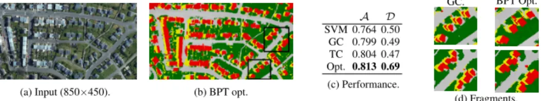
(a) Input (850×450). (b) BPT opt.

A D SVM 0.764 0.50 GC 0.799 0.49 TC 0.804 0.47 Opt. 0.813 0.69 (c) Performance. GC. BPT Opt. (d) Fragments.

Figure 5: Experimental results for the satellite image over Brest (see text for details).

images of urban scenes extracted from Google Maps. Figs.4(a) and5(a) show two color images acquired over New York City and the area of Brest, respectively. For both images, the manual segmentation was based on cadastral records available through OpenStreetMap. The list of the considered object classes is given in Fig.4(b) (no instance of the internal road class is present in the Brest image). In the particular case of buildings, cadastral information was used to delineate every object independently even when they are spatially adjacent.

To evaluate the performance of the proposed method, we use two criteria: 1) Overall accuracy A, defined as the proportion of correctly classified pixels.

2) Building’s overlap D. For every building in the manually segmented image, we search for the most overlapping building region in the segmentation map in terms of Dice’s coeffi-cient [7]. The criterion D is estimated by averaging the computed coefficients.

An SVM with a Gaussian radial basis function kernel was used for the data term, tuned by tenfold cross-validation [27]. The criterion (5) involved area, rectangularity and elon-gatedness shape descriptors. The distributions were trained on a set of sample objects from an adjacent image. In the area covered by these objects, 100 random pixels per class were selected to train the SVM.

We compared the performance of the proposed approach with the following methods: 1) SVM; 2) graph cut with α-expansion [3] (GC); 3) cut on the BPT, regularized by the number of regions without using shape priors (TC) [22]; 4) cut on the same BPT with our shape formulation (5), but without tree optimization (TSC). Figs.4(c–f) illustrate the out-put of these techniques for the image of New York. Figs.4(g–h) depict the results obtained by applying our optimization method with different values of k (see Sec. 5.2). The SVM classification exhibits many issues, notably the assignment of some roof parts to the wrong class. GC and TC smooth the results though do not correct the main mistakes in the classifi-cation. In the initial cut with shape priors on the unoptimized tree (TSC), some regions are enhanced but some others are significantly deteriorated with respect to the previous methods. This is due to the faulty tree construction that does not represent the entire objects in unique nodes. Figs.4(g–h) show that the optimization of the tree copes with these issues, not only enhancing the initial cut on the tree but also outperforming the other techniques.

The evolution of the energy (5), the accuracy A and the building’s overlap D with re-spect to the number of iterations are depicted in Figs.4(i–k). As expected, the energy curve becomes less smooth as k goes larger. For values of k small enough, the segmentation maps are almost identical. This validates the fact that many branch moves are independent and can be applied prior to reconstructing the heap.

BPT for this image is constructed in 1.25 seconds on an 8-CPU 2.7 GHz processor. The optimization time, summarized in Fig.4(l), is considerably faster with Props.1-2.

Fig.5illustrates experimental results for the image of Brest. Our method was executed with k = 600. Fig.5(b) shows the obtained segmentation map. Two fragments of the map (boxed in Fig.5(b)) are amplified for comparison in Fig.5(d). These results validate the

(11)

previous observations. The BPT is built in 13 seconds and the optimization takes 84 seconds using Props.1-2(against 214 s).

7 Conclusion

We have presented an algorithm to optimize BPTs with the ultimate goal of extracting accu-rate multi-class multi-object image segmentations with shape priors. We prune and regraft tree branches at different scales in order to minimize the energy of the best segmentation that can be extracted from a tree. Our theoretical study permits to reduce the space of branch moves.

If we see our contribution from the perspective of hierarchical partitions, we can state that our method produces better trees that represent entire objects in single nodes, a major concern reported in the BPT literature. If we see it from the perspective of class multi-object image segmentation, we can state that we have succeeded in incorporating shape information throughout the segmentation process.

In addition to being an advantageous data structure per se (because it can be reused for different goals), BPTs are a good departure point for optimization, since they allow to perform moves of variable region sizes. In an MRF approach defined on the pixel grid, each time we perform a move we would have to search for a relevant region to perform a label switch (e.g., by using minimum spanning forests). A BPT dynamically stores a set of candidate adjacent regions at different scales.

In the future, we intend to study possible extensions of the family of branch moves and their associated theoretical guarantees. We also plan to extend the number of shape features and to add hierarchical features, in order to incorporate further priors in tree enhancement and segmentation.

References

[1] Huseyin Gokhan Akcay and Selim Aksoy. Building detection using directional spatial constraints. In IGARSS, pages 1932–1935, 2010.

[2] J-M Beaulieu and Morris Goldberg. Hierarchy in picture segmentation: A stepwise optimization approach. IEEE TPAMI, 11(2):150–163, 1989.

[3] Yuri Boykov, Olga Veksler, and Ramin Zabih. Fast approximate energy minimization via graph cuts. IEEE TPAMI, 23(11):1222–1239, 2001.

[4] Felipe Calderero and Ferran Marques. Region merging techniques using information theory statistical measures. IEEE TIP, 19(6):1567–1586, 2010.

[5] Daniel Cremers, Florian Tischhäuser, Joachim Weickert, and Christoph Schnörr. Dif-fusion snakes: Introducing statistical shape knowledge into the Mumford-Shah func-tional. IJCV, 50(3):295–313, 2002.

[6] Piali Das, Olga Veksler, Vyacheslav Zavadsky, and Yuri Boykov. Semiautomatic seg-mentation with compact shape prior. Image and Vision Computing, 27(1):206–219, 2009.

(12)

[7] L. Dice. Measure of the amount of ecological association between species. Ecology, 26(3):297–302, 1945.

[8] Gareth Funka-Lea, Yuri Boykov, Charles Florin, M-P Jolly, Romain Moreau-Gobard, Rana Ramaraj, and Daniel Rinck. Automatic heart isolation for ct coronary visualiza-tion using graph-cuts. In IEEE Int. Symp. Biomedical Imaging: Nano to Macro, pages 614–617, 2006.

[9] Gonzalo Giribet. Efficient tree searches with available algorithms. Evolutionary bioin-formatics online, 3:341, 2007.

[10] L. Gorelick, F.R. Schmidt, and Y. Boykov. Fast trust region for segmentation. In CVPR 2013, pages 1714–1721, June 2013.

[11] Lena Gorelick, Olga Veksler, Yuri Boykov, and Claudia Nieuwenhuis. Convexity shape prior for segmentation. In ECCV, pages 675–690, 2014.

[12] T Kurita. An efficient agglomerative clustering algorithm for region growing. In IAPR Workshop on Machine Vision Applications, pages 210–213, 1994.

[13] Camille Kurtz, Nicolas Passat, Pierre Gancarski, and Anne Puissant. Extraction of complex patterns from multiresolution remote sensing images: A hierarchical top-down methodology. Pattern Recognition, 45(2):685–706, 2012.

[14] Victor Lempitsky, Andrew Blake, and Carsten Rother. Image segmentation by branch-and-mincut. In ECCV, pages 15–29, 2008.

[15] Fulu Li and Andrew Lippman. Random tree optimization for the construction of the most parsimonious phylogenetic trees. In CISS, pages 757–762, 2009.

[16] Huihai Lu, John C Woods, and Mohammed Ghanbari. Binary partition tree for semantic object extraction and image segmentation. IEEE Trans. Circuits and Systems for Video Technology, 17(3):378–383, 2007.

[17] Raul S Montero and Ernesto Bribiesca. State of the art of compactness and circularity measures. Int. Mathematical Forum, 4(27):1305–1335, 2009.

[18] Claudia Nieuwenhuis, Eno Töppe, and Daniel Cremers. A survey and comparison of discrete and continuous multi-label optimization approaches for the Potts model. IJCV, 104(3):223–240, 2013.

[19] Guillem Palou and Philippe Salembier. Occlusion-based depth ordering on monocular images with binary partition tree. In ICASSP 2011, pages 1093–1096. IEEE, 2011.

[20] Yossi Rubner, Carlo Tomasi, and Leonidas J Guibas. A metric for distributions with applications to image databases. In ICCV, pages 59–66, 1998.

[21] Philippe Salembier and Luis Garrido. Binary partition tree as an efficient representation for image processing, segmentation, and information retrieval. IEEE TIP, 9(4):561– 576, 2000.

[22] Philippe Salembier, Samuel Foucher, and Carlos López-Martínez. Low-level process-ing of PolSAR images with binary partition trees. In IGARSS, 2014.

(13)

[23] Bernard W Silverman. Density estimation for statistics and data analysis. CRC press, 1986.

[24] James Tilton and Edoardo Pasolli. Incorporating edge information into best merge region-growing segmentation. In IGARSS, 2014.

[25] Godfried T Toussaint. The rotating calipers: An efficient, multipurpose, computational tool. In ICCTIM, pages 215–225, 2014.

[26] Silvia Valero, Philippe Salembier, and Jocelyn Chanussot. Object recognition in ur-ban hyperspectral images using binary partition tree representation. In IGARSS, pages 4098–4101, 2013.

[27] Vlamimir Vapnik. Statistical learning theory. Wiley New York, 1998.

[28] Olga Veksler. Star shape prior for graph-cut image segmentation. In ECCV, pages 454–467, 2008.

[29] Veronica Vilaplana, Ferran Marques, and Philippe Salembier. Binary partition trees for object detection. IEEE TIP, 17(11):2201–2216, 2008.

[30] Ting-Fan Wu, Chih-Jen Lin, and Ruby C Weng. Probability estimates for multi-class classification by pairwise coupling. JMLR, 5:975–1005, 2004.

[31] Mingqiang Yang, Kidiyo Kpalma, Joseph Ronsin, et al. A survey of shape feature extraction techniques. Pattern recognition, pages 43–90, 2008.