HAL Id: hal-01453253
https://hal.archives-ouvertes.fr/hal-01453253
Submitted on 2 Feb 2017
HAL is a multi-disciplinary open access
archive for the deposit and dissemination of
sci-entific research documents, whether they are
pub-lished or not. The documents may come from
L’archive ouverte pluridisciplinaire HAL, est
destinée au dépôt et à la diffusion de documents
scientifiques de niveau recherche, publiés ou non,
émanant des établissements d’enseignement et de
A polytope-based approach to measure the impact of
events against critical infrastructures
Gustavo Daniel Gonzalez Granadillo, Joaquin Garcia-Alfaro, Hervé Debar
To cite this version:
Gustavo Daniel Gonzalez Granadillo, Joaquin Garcia-Alfaro, Hervé Debar. A polytope-based approach
to measure the impact of events against critical infrastructures. Journal of Computer and System
Sciences, Elsevier, 2017, 83 (1), pp.3 - 21. �10.1016/j.jcss.2016.02.004�. �hal-01453253�
A polytope-based approach to measure the impact of events against
critical infrastructures
G. Gonzalez-Granadillo1, J. Garcia-Alfaro1, H. Debar1
aInstitut Mines-Telecom, Telecom Sudparis, CNRS SAMOVAR UMR 5157
9 rue Charles Fourier, 91011 EVRY, France E-mails:{First Name.Last Name}@telecom-sudparis.eu
Abstract
This paper provides a method to calculate the impact of cyber attacks and security countermea-sures in a multi-dimensional coordinate system. The method considers the simulation of services, attacks and countermeasures in at least one dimensional coordinate system, the projection of which originates geometrical figures (e.g., lines, squares, rectangles, hyper-cubes). Such geometrical fig-ures are measured through geometrical operations (i.e., length, area, volume, hyper-volume), so that we determine the impact of complex attacks arriving on the system, as well as the impact of the implementation of single and/or multiple countermeasures selected to mitigate the effects of such detected attacks. As a result, we are able to measure the size of a cyber event (e.g., attack, countermeasure) over a particular system or service, making it possible to determine the percentage of the system that is under attack and the percentage of the attack that is mitigated by a given countermeasure. Suck measurements allow security administrators to determine residual risks, and potential collateral damages. A case study of a critical infrastructure is provided to show the applicability of the model.
Keywords: Geometrical Model, Polytope, Impact Measurement, Multiple Dimensions, Critical
Infrastructures, SCADA
1. Introduction
Assessing the impact of cyber attacks and countermeasures is a very challenging process that requires identifying all vulnerable elements that interact with the target system. However, the risk of potential cyber attacks cannot be accurately described unless the consequences of such attacks are properly identified and quantified. Cyber attacks may cause direct impacts that include economic loss, reputation loss, legal exposure, regulation compliance loss, potentially social impact, and even infrastructure destruction.
Estimating the impact of current cyber attacks should consider two aspects. First, the im-pact of potential mitigation actions must be considered in the simulation and analysis of cyber attack impacts. Second, the estimation of such impacts must be analyzed with respect to time, geographic space and affected elements. For small organizations, this estimation can be straightfor-ward, however, for critical infrastructures, it may pose a serious challenge. Therefore, it is of great importance to be able to quantify these impacts through the analysis of historical data or using simulation models that employ engineering, economic, or agent-based frameworks [1].
In this paper we propose a method to calculate the impact of cyber attacks and security coun-termeasures in a multi-dimensional coordinate system. The method considers ‘events’ and ‘services’ as inputs, and the impact of such events over the services as outputs. Events, e.g., attacks and countermeasures, are modeled as elements that are granted privileges over the assets of the services under multiple conditions, such as temporal conditions (e.g., granted privileges only during working hours), spatial conditions (e.g., granted privileges when connected within the company premises), and historical conditions (e.g., granted privileges only if previous instances of the same equivalent events were already conducted).
In addition, the method considers the processing of services, attacks and countermeasures in a multi-dimensional coordinate system, the projection of which originates instantiated models (e.g., n-cube, n-orthotope). Such instances are measured through geometrical operations (i.e., length, surface area, volume, hyper-volume), so that we determine the impact of complex events affecting the services. As a result, we are able to determine the portion of the service that is under attack, as well as, the portion of the attack that is controlled by a given security measure. By doing this, we automatically calculate the residual risk (the percentage of the attack that is left untreated by any countermeasure), and the potential collateral damage (the percentage of the service that is not under attack but is affected by a given countermeasure).
The rest of the paper is structured as follows: Section 2 introduces the polytope concept. Section 3 describes our proposed geometrical model and provides some examples of the possible system dimensions of the coordinate system. Section 4 presents the geometrical figures resulting from the projection of our proposed model. Section 5 discusses the geometrical operations used to measure the impact of the analyzed events. Section 6 discusses the methodology used for the model verification and validation. A case study of a critical infrastructure is presented in Section 7 to show the applicability of our model in a scenario of complex cyber attacks. Section 8 presents related works. Conclusions and Future work are presented in Section 9.
2. Polytope
In Euclidean geometry, a polytope is a geometric object with flat sides, and may exist in a general number of dimensions n as an n-dimensional polytope or n-polytope. For example, a two-dimensional polygon is a 2-polytope, and a three-two-dimensional polyhedron is a 3-polytope [2].
A polytope comprises elements of different dimensionality such as vertices1, edges2, faces3, cells4,
facets5, ridges6, etc [3] . An n-dimensional polytope is bounded by a number of (n-1)-dimensional
facets. These facets are themselves polytopes, whose facets are (n-2)-dimensional ridges of the original polytope. Ridges are once again polytopes whose facets give rise to (n-3)-dimensional
1Vertex is a special kind of point that describes the corners or intersections of geometric shapes.
2Edge is a particular type of line segment joining two vertices in a polygon, polyhedron, or higher-dimensional
polytope.
3Face is a flat (planar) surface that forms part of the boundary of a solid object; in more technical treatments of
the geometry of polyhedra and higher-dimensional polytopes.
4Cell is a polyhedral element (3-face) of a 4-dimensional polytope or 3-dimensional tessellation, or higher. Cells
are facets for 4-polytopes and 3-honeycombs.
5Facet is a feature of a polyhedron, polytope or related geometric structure, generally of dimension one less than
the structure itself.
6Ridge is a (n-2)-face of an n-polytope (also subfacet). A ridge is seen as the boundary between exactly two facets
boundaries of the original polytope, and so on. These bounding sub-polytopes may be referred to as faces, or specifically j-dimensional faces or j-faces. A 0-dimensional face is called a vertex, and consists of a single point. A 1-dimensional face is called an edge, and consists of a line segment. A 2-dimensional face consists of a polygon, and a 3-dimensional face, sometimes called a cell, consists of a polyhedron.
Polygons and Polyhedrons can be of different kinds (e.g., regular, convex, non-convex). Due to the characteristics of our coordinate system, we constrain our research to regular and closed
polytopes with right angles (equal to 90 degrees). We exclude open and irregular objects, as
well as triangles, spheres, and stars, since the projection of the entities in our coordinate system does not make possible the design of such polytopes. In addition, since the projections in our coordinate system only generates polytopes with right angles, we discard from our research rhombus, trapezoids, parallelograms, rhomboids, and other polygons with angles different from 90 degrees.
We study two basic types of polytopes: n-cubes, and n-orthotopes [3, 4] .
n-cube: It is an n-dimensional analogue of a square (n = 2) and a cube (n = 3), which has a closed, compact, convex figure whose 1-skeleton consists of groups of opposite parallel line segments aligned in each of the space’s dimensions, perpendicular to each other and of the same length. An n-cube is also called an n-dimensional hyper-cube or an n-dimensional cube.
n-orthotope: It is the generalization of a rectangle in higher dimensions, formally defined as the Cartesian product of intervals [5]. A 3-orthotope is a rectangular parallelepiped, also called a cuboid. We discard from our research the rhombohedron (a special case of parallelepiped with six rhombus faces), and all similar parallelotopes, since the projection of the axes in our coordinate system will only generate geometrical figures with right angles.
Depending on the number of dimensions, an n-cube or an n-orthotope can be one of the following: Zero dimension: A point is a hyper-cube and/or orthotope of dimension zero.
One dimension: If one moves this point one unit length, it will sweep out a line segment, which is a unit hyper-cube and/or orthotope of dimension one.
Two dimensions: If one moves this line segment in a perpendicular direction from itself; it sweeps out a 2-dimensional square or rectangle.
Three dimensions: If one moves the square one unit length in the direction perpendicular to the plane it lies on, it will generate a 3-dimensional cube. Similarly, if one moves the rectangle one unit length in the direction perpendicular to the plane it lies on, it will generate a 3-dimensional orthotope (also known as right rectangular prism, cuboid, rectangular cuboid, hyper-rectangle, orthogonal parallelepiped, or rectangular parallelepiped).
Four dimensions: If one moves the cube one unit length into the fourth dimension, it generates a 4-dimensional unit hyper-cube (a unit tesseract). Similarly, if one moves the cuboid one unit length into the fourth dimension, it generates a 4-dimensional unit orthotope.
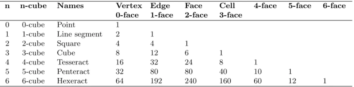
Table 1 details information about the characteristics of hyper-cubes from the zero dimensional cube up to the six-dimensional hybercube.
The information about the elements composing a hyper-cube (e.g., number of edges, faces, cells) is used in the calculation of geometrical operations (see Section 6). It is also possible to project an n-cube inside a regular 2n-gonal polygon by a skew orthogonal projection. Table 2 shows the orthographic projection from the line segment to the 6-cube.
Table 1: Hyper-cube elements
n n-cube Names Vertex 0-face Edge 1-face Face 2-face Cell 3-face
4-face 5-face 6-face 0 0-cube Point 1
1 1-cube Line segment 2 1
2 2-cube Square 4 4 1
3 3-cube Cube 8 12 6 1
4 4-cube Tesseract 16 32 24 8 1
5 5-cube Penteract 32 80 80 40 10 1
6 6-cube Hexeract 64 192 240 160 60 12 1
Table 2: n-cube orthographic projections
Line Segment Square Cube Tesseract Penteract Hexeract
It is important to note, however, that the orthographic projection of instances in more than three dimensions results into complex figures that only provides a general overview of the size and density of the represented event. It is therefore difficult to show unions and intersections from the projected events unless we restrain the graphical representation up to three dimensions.
3. Geometrical Model
In analogy with access control models [6, 7, 8], we identify three dimensions that contribute directly to the execution of a given attack e.g., User account (subject), Resource (object), and Channel (the way to execute actions, e.g., connect, read, write, etc). In addition, we use the notion of contexts proposed in the Organization based Access Control (OrBAC) model [8, 9, 10], to extend the approach into an n dimensional system, where every context will be a new dimension, such as temporal conditions (e.g., granted privileges only during working hours), spatial conditions (e.g., granted privileges when connected within the company premises), and historical conditions (e.g., granted privileges only if previous instances of the same equivalent events were already conducted). For instance, in order to access a web-server (resource) of a given organization, an external user (user account) connects remotely (spatial condition) to the system by providing his/her login and password (channel) at a given date (temporal condition). This section details five dimensions of our coordinate system. For simplicity and visualization purposes, we use a three-dimensional system to project the geometrical instances. However, it is important to note that the size of the system
is not limited to a fixed number of dimensions. Organizations must define their own dimensions to model services, and events (i.e., attacks and countermeasures).
3.1. Coordinate System
Our geometric model is proposed to represent services, attacks and countermeasures in an n-dimensional coordinate system, n being the number of dimensions (e.g, user account, channel, resource, etc). There is no limit in the number of axis composing our coordinate system. It can be a mono dimensional system (considering only one dimension), or a multi-dimensional system (considering two or more dimensions). The remaining of this section gives examples of the possi-ble dimensions that can be used to simulate attacks and countermeasures. More details of each dimension can be found in [11, 12]
3.2. User Account
A user account is a unique identifier for a user in a given system that allows him/her to connect and interact with the system’s environment. A user account is the equivalent of a ‘subject’ in an access control policy. User accounts are associated to a given status in the system, from which their privileges and rights are derived (e.g., system administrator, standard user, guest, internal user, nobody).
3.3. Resource
A resource is either a physical component (e.g., server, printer, Policy Enforcement Point-PEP) or a logical component (e.g., files, records, database) of limited availability within a computer system. Resources can be classified according to the type of user’s privilege (e.g., kernel, user), or according to the transitions performed (e.g., read, write, execute). A resource is the equivalent of an ‘object’ in an access control policy. Access to resources are either permitted or prohibited depending on the nature of the resource itself and the rights and privilege of the user that request the access.
3.4. Channel
In order to have access to a particular resource, a user must use a given channel. This latter can be an IP address, a port number, a communication protocol, an access credential, etc. A channel is the equivalent to an action in an access control policy. We consider the IP address [13, 14, 15, 16] and the port number [17, 18] to represent channels in TCP/IP connections. However, each organization must define the way its users connect to the system and have access to the organization’s resources. 3.5. Time
It expresses that a given action made by a given user on a given object is authorized only at a given time, after or before a given time, or during a given time interval. The temporal conditions can correspond to the connection time, detection time, time to react, time to completely mitigate the attack, recovery time, etc. It can refer to a day of the week, or to a time of the day. For instance, an internal user of a telecom organization may be allowed to access the database only during the working hours i.e., between 8:00AM and 19:00PM for example. Time is the equivalent to a ‘temporal context’ in an access control policy.
3.6. Location
Knowing the location from where the user makes the request can be useful to quantify the events. We can distinguish two different types of locations: physical and logical. The former corresponds to the physical location of the user, namely his/her office, a security area, a specific building, the country, etc. The latter corresponds to the ‘logical location’ he/she stands in e.g., a PC, a network or sub-network, the cell in the case of radio communication such as in UMTS, etc. Location is the equivalent to a ‘spatial context’ in an access control policy.
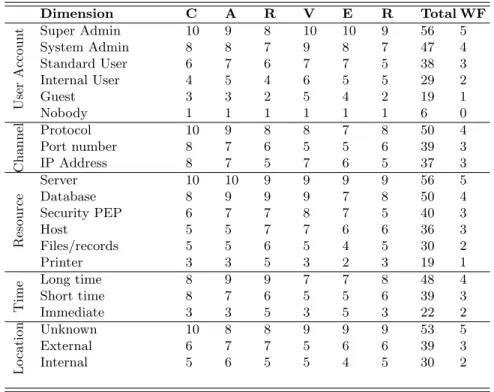
Each dimension contributes differently in the impact calculation. This contribution represents the criticality of a given element in the execution of an attack. Following the CARVER methodol-ogy [19, 20] which considers six criteria (i.e., criticality, accessibility, recuperability, vulnerability, effect, recognizability), we assign numerical values on a scale of 1 to 10 to each element within the dimension. Table 1 shows an example of this methodology implemented in the aforementioned dimensions.
Table 3: Intra-dimension Weighting Factor
Dimension C A R V E R Total WF User Accoun t Super Admin 10 9 8 10 10 9 56 5 System Admin 8 8 7 9 8 7 47 4 Standard User 6 7 6 7 7 5 38 3 Internal User 4 5 4 6 5 5 29 2 Guest 3 3 2 5 4 2 19 1 Nobody 1 1 1 1 1 1 6 0 Channel Protocol 10 9 8 8 7 8 50 4 Port number 8 7 6 5 5 6 39 3 IP Address 8 7 5 7 6 5 37 3 Server 10 10 9 9 9 9 56 5 Resource Database 8 9 9 9 7 8 50 4 Security PEP 6 7 7 8 7 5 40 3 Host 5 5 7 7 6 6 36 3 Files/records 5 5 6 5 4 5 30 2 Printer 3 3 5 3 2 3 19 1 Time Long time 8 9 9 7 7 8 48 4 Short time 8 7 6 5 5 6 39 3 Immediate 3 3 5 3 5 3 22 2 Lo cation Unknown 10 8 8 9 9 9 53 5 External 6 7 7 5 6 6 39 3 Internal 5 6 5 5 4 5 30 2
4. Resulting Geometrical Figures
A variety of geometrical figures (e.g., line segment, rectangle, square, cube) result from the analysis of the entities’ information included in a system, an attack or a countermeasure. The remaining of this section details all the different cases.
4.1. One dimension
When we have information of one dimension of our coordinate system (e.g., resources, channels, users), we project the information to obtain lines. An entity in the system represents a line segment with an origin and an end point. In order to plot an entity in the system, we need to find its coordinate. For this, we affect each entity with its associated weighting factor. This latter indicates the size of the segment, thus, the impact of the entity over the system. For instance, one regular user with limited privileges is given a weighting factor WF=2, whereas, an administrator with more privileges is given a weighting factor WF=5. The regular user will be represented in our coordinate system as a straigh line composed of two segments, whereas the administrator will be represented as a straight line composed of five segments.
These kinds of figures result when attacks or countermeasures affect one axis of our coordinate system. As a result, entities are plotted as lines in one of the axis. Several cases originate while plot-ting entities in one axis. Lines can be continuous or discontinuous. For instance, let us consider an attack that compromises a list of resources (R1:R10). Since the list includes consecutive resources, the resulting figure will be a continuous line. However, if the resource list includes discontinuous elements (e.g., R1, R7, R10), the resulting figure will be a discontinuous line composed of three segments. We discard curved lines from our research, since it is not possible to obtain them in our coordinate system.
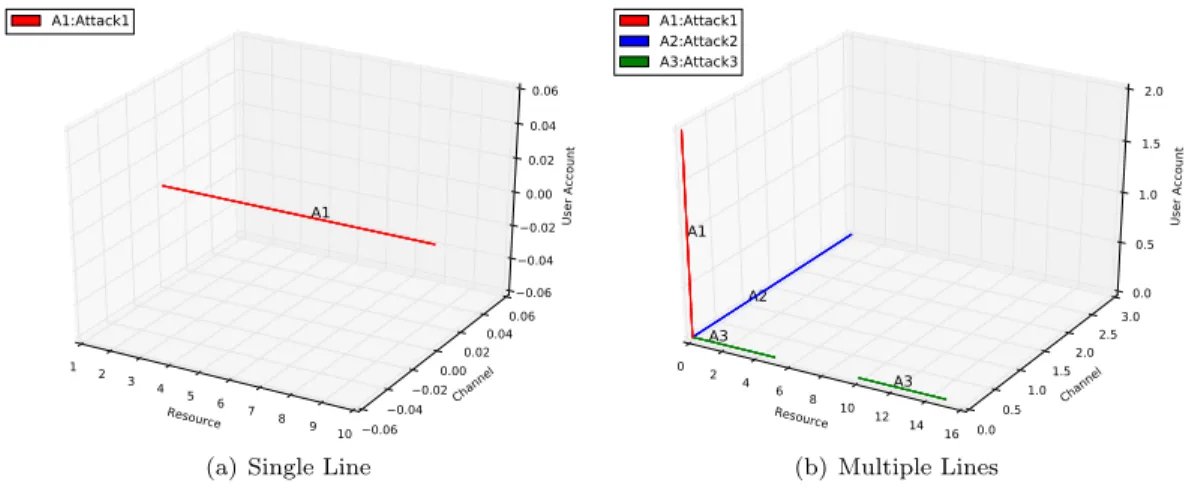
Multiple line segments originate when we detect multiple attacks against one particular dimen-sion, or when we implement countermeasures to protect one of the dimensions of our system. For instance, having attack A1 against resource R1, attack A2 against user U1, and attack A3 against channel Ch1, the resulting figure will be three disjoint lines with the same origin and with different projections.
Figure 1(a) depicts an example of an attack over a single resource (i.e., R1), with a weighting factor WF=5. Since R1 is the first entity in the resource axis, its RCU coordinate will be (0:5, 0:0, 0:0), which results into a single continuous line segment.
Resource 1 2 3 4 5 6 7 8 9 10 Channel 0.060.04 0.020.00 0.020.04 0.06 User Account 0.06 0.04 0.02 0.00 0.02 0.04 0.06 A1 A1:Attack1
(a) Single Line
Resource 0 2 4 6 8 10 12 14 16 0.00.51.0 Channel 1.52.0 2.53.0 User Account 0.0 0.5 1.0 1.5 2.0 A1 A2 A3 A3 A1:Attack1 A2:Attack2 A3:Attack3 (b) Multiple Lines
Figure 1: Graphical representation of single and multiple lines
A variant of this case will be if the incident affects several resources that do not follow a consecutive order (e.g., R1, R14, R45), in such a case, the incident will be represented graphically
as a discontinuous line composed of three segments.
Figure 1(b) shows the graphical representation of three disjoint line segments. The user axis represents a continuous line (i.e., U1) with WF=2 and RCU (0:0, 0:0, 0:2). The channel axis represents a continuous line segment (i.e., Ch1) with WF=3 and RCU (0:0, 0:3, 0:0). The resource axis represents a discontinuous line segment (i.e., R1, R3) with WF=5 and RCU (0:5&10:15, 0:0, 0:0).
4.2. Two dimensions
When we have information of two dimensions of our coordinate system (e.g., resources, channels, users), we project the information to obtain surfaces. These latter can be continuous or discon-tinuous. For instance, an attack that compromise resources R1:R10, using channel Ch2, will be represented as one continuous surface. However, if the same attack compromises resources R1, and R3, using channel Ch2, the graphical representation will be a discontinuous surface composed of two sections.
Surfaces are of two types: (1) squares, a parallelogram of four sides of equal lengths and angles of equal sides, and (2) rectangles, a parallelogram with four angles of equal sides. We discard rhomboids, rhombus, trapezoids, and other kinds of parallelograms, since they are non-right angled geometrical figures.
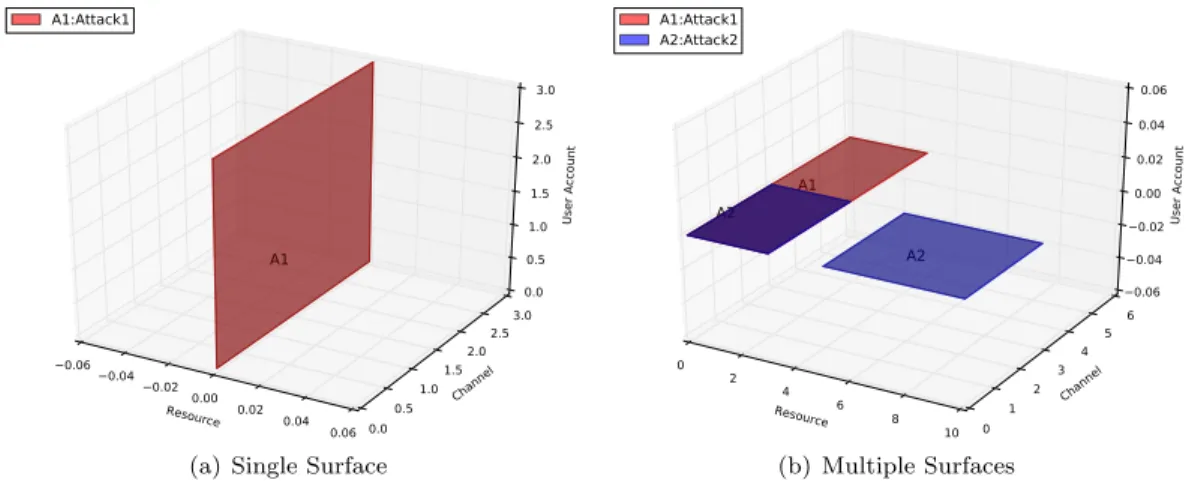
Surfaces are generated when attacks and/or countermeasures affect only two axes of our coor-dinate system. Figure 2(a) depicts the graphical representation of user U1 and channel Ch1, both entities with WF=3 (RCU 0:0, 0:3, 0:3). Since there are equal number of segments affected in each of the two axes, its projection results into a square. A variant case exists when the incident affects several entities that do not follow a consecutive order of elements, in such a case, the incident will be represented graphically as multiple surfaces (squares or rectangles).
Resource 0.06 0.04 0.02 0.00 0.02 0.04 0.06 Channel 0.00.5 1.01.5 2.02.5 3.0 User Account 0.0 0.5 1.0 1.5 2.0 2.5 3.0 A1 A1:Attack1
(a) Single Surface
Resource 0 2 4 6 8 10 Channel 0 1 2 3 4 5 6 User Account 0.06 0.04 0.02 0.00 0.02 0.04 0.06 A1 A2 A2 A1:Attack1 A2:Attack2 (b) Multiple Surfaces
Figure 2: Graphical representation of single and multiple surfaces
Figure 2(b) depicts an example of two attacks (A1 and A2) that affect RCU(0:3, 0:6, 0:0), and RCU(0:3& 5:10, 0:3, 0:0) respectively, where the ‘&’ symbol denotes a conjunctive. There is no information about the users that are affected in the incident, only the information about resources and channels is plotted. Since attack A2 covers two disjoint resources, its representation
results into two disjoint rectangles (in purple), whereas attack A1 is represented as one continuous rectangle. Considering that both attacks have some entities in common, their representation appears as partially joint surfaces.
4.3. Three dimensions
The projection of at least one entity in three dimensions results into a cube (a squared paral-lelepiped), when the length of each dimension is exactly the same, and parallelepipeds, otherwise. Cubes and parallelepipeds can be continuous or discontinuous. For instance, an attack that compro-mise resources R1:R2, users U1:U2 using channel Ch1, all elements with weighting factor WF=2 will be represented as one continuous parallelepiped. However, if the same attack compromises resources R1, and R3, user U1 and channel Ch2, all elements with weighting factor WF=2 , the graphical representation will be two disjoint cubes.
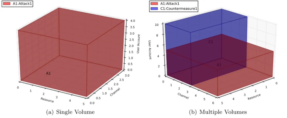
Multiple cubes and/or parallelepipeds originate when we detect one attack that affects a list of discontinuous elements from three dimensions of our coordinate system, or multiple attacks and/or countermeasures simultaneously simulated. Figure 3(a) shows the graphical representation of an incident affecting resource R1 (WF=5), channel Ch1 (WF=3), and user U1 (WF=4). The projection of these axes results into a parallelepiped. A variant of this case, results when the incident affects two or more disjoint elements, in such a case the incident is represented as multiple volumes (cubes or parallelepipeds).
Resource 0 1 2 3 4 5 Channel 0.00.5 1.01.5 2.02.5 3.0 User Account 0.0 0.5 1.0 1.5 2.0 2.5 3.0 3.5 4.0 A1 A1:Attack1
(a) Single Volume
Resource 0 1 2 3 4 5 Channel 0 1 2 3 4 5 6 User Account 0 2 4 6 8 10 A1 C1 A1:Attack1 C1:Countermeasure1 (b) Multiple Volumes
Figure 3: Graphical representation of single and multiple volumes
Figure 3(b) shows the graphical representation of multiple volumes. This case generally re-sults when plotting simultaneously several attacks and/or countermeasures that share one or more entities.
4.4. Analysis of Geometrical Figures
Events can be represented graphically as lines, surfaces (square, rectangle), and/or volumes (cube, parallelepiped). We constraint the graphical representation up to three dimensions, so that we can clearly represent the size of multiple events arriving simultaneously in the system, and therefore, we can show the overlap of joint events. We discard the representation of n-hypercubes
and n-orthotopes since their construction is complex and the visualization of multiple events in more than three dimensions will not allow security administrators to identify overlapping areas that may require updating security measures or implementing new ones.
It is important to note, however, that we can plot different geometrical figures in the same
coordinate system. If we consider, for instance, attack A1 that affects a given user; attack A2 that
affects a user and a resource; and countermeasure C1 that affects a user, a channel and a resource;
we will have as output, a line, a surface and a volume respectively. In terms of the impact of each event, the higher the number of affected dimensions, the higher the size of the event, and thus, the higher its impact. An attack that is represented as a surface will generally have a higher priority than another attack that is represented as a line. Similarly, an attack that is represented as a volume, will have a higher priority than another one represented as a surface or a line.
The representation of security measures has a double effect: On the one hand, if the counter-measure is too small compared with the attack, the residual risk will be too high, since a big portion of the attack will be untreated by the countermeasure; on the other hand, if the countermeasure is too big with respect to the attack, the potential collateral damage will be too high, since a big portion of the system or service that is not under attack will be affected by the countermeasure. It is therefore important to accurately measure the size of each event while plotting them in the co-ordinate system, since that will set up the reaction strategies that will be implemented to mitigate the effects of a given attack.
The fact that a security measure is too big with respect to the attack does not imply that the attack is totally covered. The coverage of events with respect to the service is a measurement that is automated in our approach. Such coverage is of vital importance in the evaluation and analysis of multiple countermeasures against complex cyber attacks. We propose to use two axioms in order to compute the risk mitigation level of multiple security measures. When two or more countermea-sures are analyzed, we should consider the costs and benefits of their implementation.
Axiom 1 The cost of a combined countermeasure is equal to the sum of all individual
counter-measure’s cost (Equation 1), where ARC is the countermeasure cost and C1, C2 are the individual
countermeasures.
ARC(C1∪ ... ∪ Cn) = ARC(C1) + ... + ARC(Cn) (1) This axiom is used for joint and disjoint countermeasures, with a pessimistic approach, since the enforcement of multiple countermeasures generally implies higher costs of implementation, consult-ing, maintainconsult-ing, etc, compared to the costs incurred out of the enforcement of a single solution. In other words, if the solution is effective for a higher cost, it will still be effective if the cost is lesser than the one estimated.
Axiom 2 The Risk Mitigation (RM) for a combined solution is calculated by adding the effec-tiveness of countermeasures over the different surfaces they cover. For two disjoint countermeasures
(e.g., C1,C2), RM is calculated as the sum of the individual coverage (Cov) times its associated
effectiveness (EF), i.e., RM (C1∪ C2) = Cov(C1)× EF1+ Cov(C2)× EF2. However, for two joint
countermeasures, RM can be calculated as the sum of their individual Coverage (Cov) times the Ef-fectiveness Factor minus the Coverage of their intersection times the minimum EfEf-fectiveness Factor (Equation 2).
RM (C1∪ C2) = Cov(C1) × EF1+ Cov(C2) × EF2
−Cov(C1∩ C2) × min{EF1, EF2}
(2)
A countermeasure coverage represents the level of action that a security solution may have on a system’s attack surface. This latter is defined in [21, 22, 23] as the subset of the system’s resources that a malicious entity may use to send/receive data into/from the system to attack the system. Thus, the more exposed the system’s surface, the more attack opportunities and hence, the more likely the system will be a target of attack [24, 25].
The union of two or more countermeasures results in an index that ranges from the maximum
coverage of the group of countermeasures (e.g., max{Cov(C1) ,..., Cov(Cn)} in its lower bound,
to the sum of the individual countermeasures (e.g., PCov(C1),...,Cov(Cn)) in its upper bound.
The intersection of two or more countermeasures is an index that ranges from zero in its lower bound, to the minimum coverage of the group of countermeasures in its upper bound (e.g., min
{Cov(C1),...,Cov(Cn)}).
Two cases can be distinguished in the calculation of the coverage for a combined countermeasure (e.g., joint and disjoint surfaces).
Disjoint Countermeasures: Two or more countermeasures are disjoint if they have no
elements in common. Therefore, having two disjoint countermeasures (C1, C4), the coverage
of the union is calculated as Cov(C1∪ C4) = Cov(C1) + Cov(C4), and the coverage of the
intersection is equal to zero.
Joint Countermeasures: Two or more countermeasures are joint if they have at least one element in common. One countermeasure can be partially or totally covered by another one. For partially covered countermeasures, the union of the combined solution is calculated as the sum of the individual surfaces minus their intersection (Equation 3), and the coverage of the intersection is approximated as the average of the lower and upper bounds (Equation 4).
Cov(C1∪ C2) = Cov(C1) + Cov(C2) − Cov(C1∩ C2) (3)
Cov(C1∩ C2) ∼=
Cov(C1∩ C2)LOW+ Cov(C1∩ C2)U P
2 (4)
The lower bound of the intersection between two countermeasures is equal to zero if the sum
of their coverage is lesser or equal to one; and it gets the value of (Cov(C1) + Cov(C2) − 1)
otherwise (Equation 5). Cov(C1∩ C2)LOW = if Cov(C1) + Cov(C2) 6 1 → 0 if Cov(C1) + Cov(C2) > 1 → Cov(C1) + Cov(C2) (5)
The upper bound of the intersection between two countermeasures is equal to the total cov-erage of the smallest countermeasure (Equation 6).
Cov(C1∩ C2)U P = min {Cov(C1), Cov(C2)} (6) When analyzing multiple geometrical figures we need to first identify if they are joint or disjoint. In case they are joint, we need to determine the coverage level. If this latter is 100%, it means that one event is totally covered by another, but it will never means that both events will have the same impact. For this, it is necessary to select one geometrical operation (discussed in Section 5) to be computed for both events, and then, if the results are the same (even if the events are disjoint), we
can say that both events have the same impact. For instance, let us assume that attack A1 affects
user U1:U5 (all of them regular users with weighting factor WF=1), and attack A2affect user U100
(an administrator with WF=5). The length of both attacks will be 5 units, and therefore, they will be considered as events with the same impact over the system.
If two or more attacks are partially covered, we need to compute the overlapping area in order to determine the impact of the joint attack over the system. The same applies for countermeasures. However, if one attack and one countermeasure are partially joint, we compute the overlapping area to determine the percentage of the attack that is covered by the countermeasure, as well as, the residual risk and the potential collateral damage.
The ultimate goal of this graphical representation is to avoid overlapping problems while plotting multiple events in the same coordinate system. This is solved by using the aforementioned axioms in the evaluation of multiple security countermeasures. By doing this, we can set up appropriate reaction strategies that mitigate the effects of complex and multiple cyber attacks, while keeping, at the same time, the best financial response for the organization.
5. Geometrical Operations
This section details the calculation of the measurements (i.e., length, area, volume, hyper-volume) [26, 27, 28] of the different geometrical figures described in the previous section. Such measurement allows us to calculate the impact of each event in the system.
5.1. Length L(X)
Working on one dimension, we can calculate the length (L) of each entity as the product of the number of elements and their associated weighting factor. Results are expressed in unit(s), using Equation 7.
L(X) = Q(E) × W F (E) (7)
where Q(E) is the number of elements that belong to the entity, and W F (E) is the weighting factor of the element.
For instance, an attack “A1” that affects resources (R1:R10), all with a weighting factor WF=5, will have a segment length equals to L(A1)= 50 units. Another example can be an attack that affects users (U1, U3, U7), weighting factor WF=2, WF=3, and WF=5 respectively. The length of the attack is therefore L(A1)= (1 × 2)+(1 × 3)+(1 × 5)= 10 units.
We discard the arc length from this type of operations, since we can only obtain straight lines from the geometric figures of our approach. Curved lines are not possible to be drawn in tour coordunate system. Geometrical operations (e.g., union, intersection) are possible if the concerned entities belong to the same axis, otherwise, no possible operation can be made. However, if one
entity (e.g. A1) is projected in one axis, and another entity (e.g., A2) is projected in two or three axis (including the axis of A1), it is still possible to perform geometrical operations as long as as long as we calculate the perimeter (P) of the geometrical figure using one of the following equations:
P (Square) = 4L(X) (8) P (Rectangle) = 2L1(X) + 2L2(X) (9) P (Cube) = 12L(X) (10) P (Cuboid) = 4L1(X) + 4L2(X) + 4L3(X) (11) P (Hyper − cube) = En× L(X) (12) P (Hyper − cuboid) = 4(L1(X) + L2(X) + ... + Ln(X)) (13)
where L is the length of one side of the entity (using Equation 1); L1, L2, L3, ..., Ln the length of
each side of the entity; and En is the number of edges of the hyper-cube. For instance, a tesseract
(4-cube) has 32 edges, whereas a penteract (5-cube) has 80 edges.
Let us consider that attack A1 against user U1 is projected as a continuous line, and counter-measure C1 is used to protect resources (R1:R3) and users (U1:U5). The resulting figure of C1 is a surface. Assuming that all affected elements have the same weighting factor (WF=2), we calculate the area of both entities (i.e., A1, and C1). For A1, the area will be A(A1)= (1 × 2) = 2 units. Since C1 is a rectangle, the length will be L(C1)= 2(3 × 2) + 2(2 × 2) = 20 units.
5.2. Area A(X)
We calculate the surface area of a square or a rectangle as the product of its length and its width (we exclude the area of circles, ellipses, trapezoids, parallelograms, and all irregular polygons, since
it is not possible to obtain such geometric figures in our approach). Results are expressed in units2,
using Equation 14.
A(X) = (Q(E)Axis1× W F (E)Axis1) × (Q(E)Axis2× W F (E)Axis2) (14)
For instance, an attack A1 that affects resources R1, R3 (WF=5) and channel Ch1, Ch2 (WF=3)
will have an area equal to A(A1)= (2×5) × (2×3) = 60 units2. Geometrical operations are possible
if the entities are represented within the same axes. For instance, if attack A1 affects users and channels, a valid countermeasure should apply to at least one of the affected users and channels.
A variant of the previous case results when having attack A1 (with the same characteristics as presented previously) and countermeasure C1 that protects resources R1:R5 (WF=4), channels Ch1:Ch5 (WF=3), and users U1:U5 (WF=2). In this case, the attack is represented in two dimen-sions (as a rectangle), and the countermeasure is represented in three dimendimen-sions (as a cuboid). It is still possible to perform geometrical operations as long as we calculate the surface area (A) of the geometrical figure using one of the following equations:
A(Square) = L2(X) (15) A(Rectangle) = L1(X) × L2(X) (16) A(Cube) = 6L2(X) (17) A(Cuboid) = 2(L1(X) × L2(X)) + 2(L1(X) × L3(X)) + 2(L2(X) × L3(X)) (18) A(n − cube) = F n × L2(X) (19) A(n − orthotope) = 2(L1(X) × L2(X)) + L1(X) × L3(X) + ... + L1(X) ×Ln(X) + L2(X) × L3(X) + ... + Ln−1× Ln) (20)
Note that from Equation 13, F n refers to the number of faces of the hyper-cube. For instance, a tesseract (4-cube) has 24 faces, whereas a penteract (5-cube) has 80 faces.
Following the previous example, the area of countermeasure C1 (cuboid) is calculated using Equation 12.
L1(X) = (Q(E)Axis1×W F (E)Axis1)×(Q(E)Axis2×W F (E)Axis2) = (5×4)×(5×3) = 300units
L2(X) = (Q(E)Axis2× W F (E)Axis2) × (Q(E)Axis3× W F (E)Axis3) = (5 × 3) × (5 × 2) = 150units
L3(X) = (Q(E)Axis1× W F (E)Axis1) × (Q(E)Axis3× W F (E)Axis3) = (5 × 4) × (5 × 2) = 200units
As a result, the area of countermeasure C1 is equivalent to A(C1)= 2(300×150) + 2(150×200)
+2(300×200) = 270,000 square units (units2), and its length is equivalent to L(C1) = 4(300) +
4(150) + 4(200) = 2,600 units. Note that the surface area of a line can be calculated as the length (L) of the line times one unit (empty axis are filled with one unit).
5.3. Volume V(X)
The volume of a given entity is calculated as the product of their elements and their associated
weighting factor, as shown in Equation 21. We exclude the volume computation of cylinders,
pyramids, cones, spheres, ellipsoids, and all irregular prisms, since it is not possible to obtain such
geometrical figures from our approach. Results are expressed in cubic units (units3).
V (X) = (Q(E)Axis1× W F (E)Axis1) × (Q(E)Axis2× W F (E)Axis2)
×(Q(E)Axis3× W F (E)Axis3) (21)
For instance, an attack A1 that affects resources R1, R3, (WF=5), channel Ch2 (WF=3), and
users U1, U2, U3 (WF=2), will have a volume equal to V(A1) = (2×5)×(1×3)×(3×2)= 180 units3.
A variant of this case results when having an entity (e.g., attack) represented in three dimensions (volume) and another entity (e.g., countermeasure) represented in one, two, four or more dimensions. It is still possible to perform geometrical operations as long as we calculate the volume (V) of the geometrical figure using one of the following equations:
V (Cube) = L3(X) (22)
V (Cuboid) = L1(X) × L2(X) × L3(X) (23)
V (n − cube) = Cn× L3(X) (24)
V (n − orthotope) = L1(X) × L2(X) × L3(X) + L1(X) × L2(X) × L4(X) + ... + L1(X) × L2(X)
Note that from Equation 18, Cn refers to the number of cells of the hyper-cube. For instance, a tesseract (4-cube) has eight cells, whereas a penteract (5-cube) has 40 cells.
Having attack A1 affecting elements: R1:R3 (WF=4), Ch1:Ch4 (WF=3), U1:U12 (WF=1), and T1:T6 (WF=2), T being a fourth dimension (e.g., time); we use Equation 18 to calculate the
volume of Attack A1 (a 4-hyper-cube) as: V(A1)= 8(3×4)3 = 13,824 units3. The area of attack
A1 is calculated using Equation 13 as A(A1)=24(3×4)2 = 3,456 units2, and the length of attack
A1 is calculated using Equation 4 as L(A1) = 12(4×3) = 144 units.
Regarding geometrical operations, intersection is possible if the entities are represented within the same axes and there is at least one element in common in each axis. Otherwise, only the union of entities can be calculated.
Note that the volume of a line, square and rectangle can be calculated as the total surface area (A) of the line, square and rectangle times one unit (empty axis are filled with one unit).
5.4. Hyper-volume
The measurement of a hyper-cube or an orthotope can be performed through the calculation of
their hyper-volume [27] (in unitsn), volume (in units3), area (in units2), or length (in units). The
hyper-volume of an entity ‘E is calculated as the product of their elements and their associated weighting factor (for each axis), as shown in Equation 26. We exclude from this operation, the hypervolume of hyperprisms, hypercylinder, and irregular orthotopes, since it is not possible to
obtain such figures from our approach. Results are expressed in unitsn.
H(X) = (Q(E)Axis1× W F (E)Axis1) × ... × (Q(E)AxisN −1× W F (E)AxisN −1)
×(Q(E)AxisN× W F (E)AxisN) (26)
For instance, an attack A1 that affects resources R1, R3, (WF=5), channel Ch2 (WF=3), users U1, U2 (WF=2), at Time T1, T2, T5 (WF=4), will have a hyper-volume equal to H(A1) = (2×5)
× (1×3) × (2×2) × (3×4)= 1,440 units4.
A variant of this case originates when having an entity (e.g., attack) represented in a given dimension (4 dimensions) and another entity (e.g., countermeasure) represented in a different di-mension (e.g., 2, 5 or more didi-mensions). In such a case we need to normalize all entities to work in the same dimensional coordinate system as explained before.
It is still possible to perform geometrical operations as long as we calculate the hyper-volume (H) of the geometrical figure using one of the following equations:
H(n − cube) = Ln(X) (27)
H(n − orthotope) = L1(X) × L2(X) × ... × Ln(X) (28)
Note that the hyper-volume of the rest of the geometrical figures is calculated as its
correspond-ing volume times one unitn−3 (empty axis are filled with one unit).
In a 4-dimensional coordinate system, for instance, attack A1 affects resource R1, channel Ch1, user U1, at Time T1. Assuming that all the elements have a weighting factor WF=2, Attack A1 is
therefore represented as a tesseract (4-cube), whose hyper-volume is calculated as: H(A1)=(1×2)4
= 16 units4. The volume of the same attack is calculated as V(A1)=8×(1×2)3 = 64 units3, its
total area corresponds to A(A1)=24×(1×2)2 = 96 units2, and its length is equivalent to L(A1) =
5.5. Analysis of Geometrical Operations
As previously described, we propose to compute the impact of events over services based on
their size in the coordinate system. The size of an event depends on the number of affected
elements and the importance of such elements to the execution of the organization’s objectives. Such importance is measured based on a multi-criteria methodology that considers the criticality, accessibility, recuperability, vulnerability, effect, and recongnizability.
Vulnerable elements are organized in one or more axes of the coordinate system. Therefore, if affected elements belong to only one axis, we propose to compute their length; if they belong to two axes, we propose to compute their area in the plane; if they belong to three axes, we propose to compute their volume; and if they belong to four or more axes, we propose to compute their hyper-volume. We do not consider the computation of the following measurements [29]: Angles (measurement of a change in direction or orientation, e.g., radian), weight (the amount of matter mass in an object, e.g., Kilogram), time (the duration of an event, e.g., seconds), temperature (the average energy per degree of freedom of a system, e.g., kelvin), since they do not provide a comparable measurement of the impact of the different events, and most of them cannot be computed due to the constraints and characteristics of the geometrical figures.
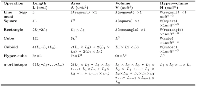
Table 4 summarizes the different measurements propose to compute the impact of events over services.
Table 4: Summary of Geometrical Operations
Operation Length Area Volume Hyper-volume L (unit) A (unit2) V (unit3) H (unitn)
Line Seg-ment
L L(segment) ×1 A(segment) ×1 V(segment) ×1 unitn−3
Square 4L L2 A(square) ×1 V(square)
×1unitn−3
Rectangle 2L1+2L2 L1× L2 A(rectangle) ×1 V(rectangle) ×1unitn−3 Cube 12L 6L2 L3 V(cube) ×1unitn−3 Cuboid 4(L1+L2+L3) 2(L1× L2) + 2(L1× L3) + 2(L2× L3) L1 × L2 × L3 V(cuboid) ×1unitn−3 Hyper-cube En×L Fn×L2 Cn×L3 Ln n-orthotope 4(L1+L2+...+Ln) 2(L1× L2 + L1× L3 +...+ L1× Ln + L2× L3 +...+ Ln−1× Ln) L1× L2× L3 + L1× L2 × L4 +...+ L1 × L2×Ln + L2×L3×L4 +...+ Ln−2× Ln−1× Ln L1× L2× ... × Ln
En: number of edges of the hyper-cube F n: number of faces of the hyper-cube Cn : number of cells of the hyper-cube
Results are expressed in unitsn, n being the number of axes that contain the affected elements.
For instance, lengths are expressed in units, since only one axis is affected; areas are expressed in
units2, since two axes are affected; volumes are expressed in units3, since three axes are affected.
Hypervolumes, however, can be expressed in units4, units5, ..., unitsn, depending on the number
It is important to note that even though the graphical representation of events and services is limited to three dimensions, we do not constrain the number of axes in the impact calculation, which could go up to the nth dimension, as long as we have information of the affected dimensions. We can compare the impact of two events based on their size. However, we need to use the
same unit-scale in the analysis. For instance, if attack A1 is a cube, whose size is expressed in
units3, and attack A2 is a hyper-cube whose size is expressed in units4, we can refer to Table 4
to use the appropriate equations to normalize both attacks into the same unit system. We can
for instance, compute the volume (units3) of the hyper-cube, or the hyper-volume (units4) of the
cube. Regardless of the selected approach, we need to normalize the results before analyzing them. Once the normalization process takes place, we can compare attacks and countermeasures in size and, therefore, in terms of their impact on the system.
After determining the size of events, we can assign priorities, for instance, we can decide which attack should be treated first and which one later. We can also decide if two or more attacks need to be treated simultaneously. In addition, we can identify which countermeasure is more suitable to react against the group of detected attacks, or if it is necessary to implement more than one security measure to mitigate them all.
The benefits of quantifying the size of services and events are multiple. first, we can compute the impact of events over the system. Second, we can analyze multiple events and assign priorities to those with higher impact. Third, we can set up reaction strategies that may include the selection of multiple countermeasures against a given attack scenario. Forth, we can propose geometrical equations to compute the union and intersection of multiple events based on their size and not on estimated values. Fifth, we can accurately identify the size of the system under attack, the residual risk and the potential collateral damage.
6. Model Verification and Validation
Model verification is defined as the process of determining that a model implementation and its associated data accurately represent the developer’s conceptual description and specifications, whereas model validation is defined as the process of determining the degree to which a simulation model and its associated data are an accurate representation of the real world from the perspective of the intended uses of the model [30].
Before running test cases for verification and validation (V&V) we defined the following list of functional requirements for our model:
R-1: the model must perform all computations in a reasonable time, R-2: the model must be able to scale,
R-3: the model must generate a graphical representation of services, R-4: the model must generate a graphical representation of events, R-5: the model must compute the impact of events,
R-6: the model must be able to automatically compute the coverage of selected events, R-7: the model must compute the risk mitigation level of countermeasures,
R-8: the model must compute the residual risk,
R-9: the model must compute potential collateral damage.
In order to ensure that the model has been built according to the requirements and design specifications, and that it meets the user’s needs, we performed a general working pattern for the verification and validation of functional requirements based on different approaches from the literature [31, 32, 33]. We applied the following methodology to our model:
1. Syntactic functionality check: It checks the existence of a piece of code that should implement the functionalities needed to cover the defined requirement. For instance, let us consider the requirement R-6 “The model must be able to automatically compute the coverage of selected events”. This functionality is implemented by two methods: (i) ComputeAttackCoverage(), which uses the classes IndividualAttackCoverage, and CombinedAttackCoverage to compute the percentage of a service that is compromised by an attack or a group of attacks; and (ii) ComputeCountermeasureCoverage(), which uses the classes IndividualCountermeasureCover-age, and CombinedCountermeasureCoverage to compute the percentage of an attack (or a group of attacks) that is mitigated by individual or combined countermeasures.
2. Semantic functional check: It checks that the corresponding implementation of the require-ment is correct with respect to its semantic (i.e., the model behaves as it is supposed to do for the given inputs). This can be done by using black box tests on the subset of identi-fied methods/classes and comparing expected input/output pairs with actual input/output pairs. Input should be selected in order to test valid values, invalid values, boundary con-ditions, exceptional cases etc. Considering again R-6, we check the implementation of the method ComputeCountermeasureCoverage() by creating different objects (valid, not valid, empty, etc..), writing by hand the expected corresponding coverage result and then checking the actual results produced by the module. Results show that for valid input (i.e., numerical and positive values of the quantities and weighting factor of users, channels, resources and all other elements composing the coordinate system), the model provides a positive and numeri-cal value (between zero and one) of the coverage of selected events, however, for invalid input (e.g., alphabetical characters, negative values, especial characters, etc.), as well as empty in-put, the model provides an error message indicating that it is unable to process the input information.
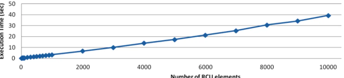
3. Effectiveness functional check: The aim of this check is to verify the “goodness” of the imple-mentation with respect to some specified quality parameters (e.g., performance, scalability, accuracy). The test definition deeply depends on the nature of the implementation and can be different case by case. We performed a set of test cases (human tests e.g., code inspection, design inspection, etc., and computer-based tests e.g., black box test, white box test, etc.), where we checked the effectiveness of the model. For instance, we run over 500 tests to eval-uate the performance of our model (in terms of processing time) by changing the number of elements to be computed from 1 to 10,000. Results are shown in Figure 4.
In order to compute the user’s request, the system needs to undertake three steps: (i) Obtain the input elements e.g., Resources (R), Channels (C), Users (U) that match with the user’s request; (ii) Compute the impact of the event; (iii) plot the graphical representation of the event. Figure 4 shows that the performance of the model goes from 0.36 seconds when plotting an event that affects a single resource, channel and user (i.e., R1,C1,U1), to 39.35 seconds when plotting an event that affects 10,000 resources, channels and users (i.e., R1:R10000, C1:C10000, U1:U10000). As a result, we can observe that the system does not degrade with high volumes of data, keeping the processing time under reasonable values.
7. Use case: Energy Distribution
We study the infrastructure environment of an Energy Distribution organization. The envi-ronment consists of a distributed network of Remote Terminal Units (RTU) in energy stations of medium voltage (MV = 20,000 Volts) and high voltage (HV = 150,000 Volts), that acquire data from electrical equipments (e.g., PLC, sensors, etc), and send them to the Supervisor Terminal Unit (STU) of the headquarters.
The system uses Supervisory Control and Data Acquisition (SCADA) protocols. The SCADA network is composed of over 13,000 energy stations, 6,000 of which are controlled by the central system.
The operating environment consists of three main parts, namely:
1. Supervisor Terminal Unit (STU): the component used to acquire data from remote stations; 2. Gateway Front-End (FE) RTU: the components that allow communications through different
types of media;
3. Remote Terminal Units (RTU): remote systems for the acquisition and control of electrical equipment.
The main STU communicates with the FE RTUs, which in turn establish the connection with the RTU substation of energy. The geographical connection between the FE RTU and the RTU occurs with different types of media (e.g., fiber optic, leased line, PSTN, GSM). At the same time the RTU of substation can communicate with each other through links, geographical Hyperlan, or LTE to exchange status, receive alarms or to send commands.
The Human Machine Interface (HMI) is linked to the SCADA system’s databases and software programs, to provide trending, diagnostic data, and management information such as scheduled maintenance procedures, logistic information, detailed schematics for a particular sensor or machine, and expert-system troubleshooting guides. In the absence of security compromise, operators review the security status of the Monitored System (SCADA and ICT environment). Security status indicators may note the presence of one or more system vulnerabilities due to known software security flaws as posted by publicly available vulnerability advisory services. Attack paths from hypothetical attack sources to known mission critical systems are analyzed and the impact on critical business functions (e.g., energy distribution) is assessed resulting in a quantified risk assessment. 7.1. Simulation Environment
The simulation environment of the organization (Sim-Env for short) contains physical and virtual machines, and emulates as much as possible the geographical wide area (WAN) links between Servers and Remote Substations using real and emulated WAN router devices. The real SCADA applications are running on devices, therefore, the Sim-Env performs the same Command and
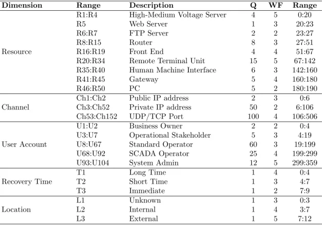
Control functionality that the Energy Distribution System has within the critical infrastructure electrical distribution equipment. The Sim-Env includes real (non-operative) Servers/Hosts and real remote stations. For testing purposes, a list of the elements composing each dimension of our coordinate system is provided in Table 5.
Table 5: Coordinate System Information
Dimension Range Description Q WF Range
R1:R4 High-Medium Voltage Server 4 5 0:20
R5 Web Server 1 3 20:23
R6:R7 FTP Server 2 2 23:27
R8:R15 Router 8 3 27:51
Resource R16:R19 Front End 4 4 51:67
R20:R34 Remote Terminal Unit 15 5 67:142
R35:R40 Human Machine Interface 6 3 142:160
R41:R45 Gateway 5 4 160:180
R46:R50 PC 5 2 180:190
Ch1:Ch2 Public IP address 2 3 0:6
Channel Ch3:Ch52 Private IP address 50 2 6:106
Ch53:Ch152 UDP/TCP Port 100 4 106:506
U1:U2 Business Owner 2 2 0:4
U3:U7 Operational Stakeholder 5 3 4:19
User Account U8:U67 Standard Operator 60 3 19:199
U68:U92 SCADA Operator 25 4 199:299
U93:U104 System Admin 12 5 299:359
T1 Long Time 1 4 0:4
Recovery Time T2 Short Time 1 3 4:7
T3 Immediate 1 2 7:9
L1 Unknown 1 3 0:3
Location L2 Internal 1 4 3:7
L3 External 1 5 7:12
7.2. Attack Scenario
Three vulnerabilities (i.e., CVE 1999-0510, CVE 1999-0618, CVE 1999-0651) have been ex-ploited by attack A1 in all host terminals, (i.e., R46:R50). The first vulnerability affects all vulner-able routers from the system (i.e., R8:R15), making it possible for a router to allow source routed packets from such hosts. IP packets sent over the Internet are normally sent between different routers to reach their final destination. The route each packet takes is determined dynamically by each router along the way. Enabling the source routing option on an IP packet allows the packet to make known to each router the path it wishes to take to reach its final destination [34].
By routing packets through a path that bypasses filtering routers and other normal security mechanisms, an attacker is able to reach a host that normally could not be reached. In addition, since the source route option causes the IP addresses in the datagram to change as the datagram
traverses the network, it is used to bypass authentication mechanisms that rely on the source IP address for access control. Using source routing, the intruder bypasses firewalls and other perimeter defense mechanisms.
The second vulnerability runs commands on remote computers running the Rexec service (a system daemon). The Rexec service authenticates the user name on the remote computer before executing the specified command [35]. The third vulnerability allows users to login to the host remotely without providing a password [36].
Attack A1 has been detected to be originated from an outside network (i.e., L3), and has partially affected the system’s confidentiality (e.g., there is considerable informational disclosure), integrity (e.g., modification of some system files or information is possible, but the attacker does not have control over what can be modified, or the scope of what the attacker can affect is limited), and availability (e.g., there is reduced performance or interruptions in resource availability), resulting in a Common Vulnerability Score System (CVSS) impact score of 6.4 (i.e., medium impact) for the first vulnerability, 10.0 (i.e., high impact) for the second vulnerability, and 7.5 (i.e., medium impact) for the third vulnerability. This score can be used to evaluate impacts and compare them
with the size (unitsn) of each event in order to set up reaction strategies.
If attack A1 succeeds, the system will require a short time to recover (i.e., T2). Attack A1 affects the following channels: four private IP addresses (i.e., Ch5:Ch8), twelve UDP Ports (i.e., Ch61:Ch72), and six TCP Ports (i.e, Ch140:Ch145); and the following user accounts: two system admin (i.e., U93:U94), and 50 standard operators (i.e., U8:U57).
The contribution of each dimension for attack A1 is computed as follows:
L1(resource) = (8×3)+ (5×2) = 34 units
L2(channel)= (4×2) + (12×4) + (6×4)= 80 units
L3(user)= (50×3) + (2×5) = 160 units
L5(location)= 1×5 = 5 units
L5(recovery time)= 1×3 = 3 units
Using Equation 22, we calculate the hyper-volume of attack A1 (5-orthotope).
H(A1) = 34units × 80units × 160units × 5units × 3units× = 6, 528, 000units5
We can also calculate other geometrical measurements of attack A1, such as the perimeter (Equation 7), the area (Equation 14), and the volume (Equation 19).
P(A1) = 4(34+80+160+5+3)= 1128 units
A(A1) = 2((34×80)+ (34×160)+(34×5)+(34×3)+(80×160)+(80×5)+(80×3)+(160×5)+(160×3)
+ (5×3) = 46,334 units2
V(A1) = (34 × 80× 160)+ (34 × 80× 5)+(34 × 80× 3)+(34 × 160× 5)+(34 × 160× 3)+(34 ×
5× 3)+(80 × 160× 5)+(80 × 160× 3)+(80 × 5× 3)+(160 × 5× 3)= 606,990 units3
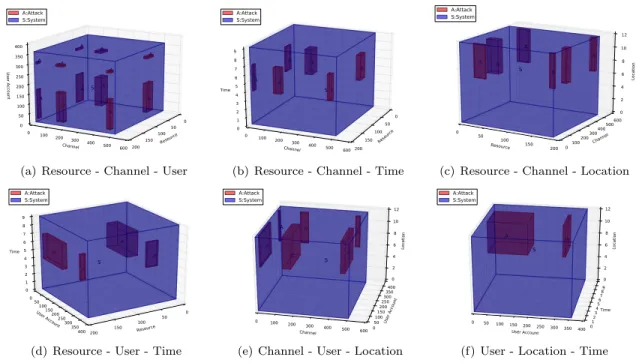
Figure 5 depicts the graphical representation of the attack impact over the Sim-Env System. This latter is represented as a continuous blue cuboid, whereas attack A1 is represented as discontinuous red cuboids that are inside the Sim Env representation. We provide different views of the graphical representation of A1 and Sim-Env, by selecting three dimensions at a time. For instance, Figure 5(a) shows the graphical representation of attack A1 and Sim-Env system based on the information about the affected resources, channels and users. Figure 5(b) includes the information of affected resources and channels vs. the system’s recovery time. Figure 5(c) depicts the graphical representation of
the affected resources and channels, vs. the attacker’s location. Figure 5(d) shows the graphical representation of the affected resources and users, vs. the system’s recovery time. Figure 5(e) shows the graphical representation of the affected channels and users, vs. the attacker’s location. Figure 5(f) shows the graphical representation of the affected users, vs. the attacker’s location and the recovery time. Resource 0 50 100 150 200 Channel 0 100 200 300 400 500 600 User Account 0 50 100 150 200 250 300 350 400 A A A A A A A A A A A A S A:Attack S:System
(a) Resource - Channel - User
Resource 0 50 100 150 200 Channel 0 100 200 300 400 500 600 Time 0 1 2 3 4 5 6 7 8 9 A A A A A A S A:Attack S:System
(b) Resource - Channel - Time
Resource 0 50 100 150 200 0100 Channel 200300 400500 600 Location 0 2 4 6 8 10 12 A A A A A A S A:Attack S:System
(c) Resource - Channel - Location
Resource 0 50 100 150 200 User Account 050 100150 200250 300350 400 Time 0 1 2 3 4 5 6 7 8 9 A A A A S A:Attack S:System
(d) Resource - User - Time
Channel 0 100 200 300 400 500 600050 User Account 100150 200250 300350 400 Location 0 2 4 6 8 10 12 A A A A A A S A:Attack S:System
(e) Channel - User - Location
User Account 0 50 100 150 200 250 300 350 400 Time 01 23 45 678 9 Location 0 2 4 6 8 10 12 A A S A:Attack S:System
(f) User - Location - Time
Figure 5: Graphical Representation of the Attack Impact in three dimensions
Depending upon the dimensions we select to be plotted, we will have a higher or lesser number of cuboids inside the Sim-Env. In five dimensions, we can show up to ten graphical representations of the same attack in a 3D coordinate system. Such representations provide different views of the attack’s impact over the studied system.
7.3. Countermeasure Analysis
Countermeasures consist of one or more discrete actions that collectively improve the security status of the monitored system (e.g., patch deployment or other system reconfiguration). Counter-measures are selected and executed by security operators, resulting in their automated deployment where possible (e.g., equipment reconfiguration) or otherwise, issuing instructions to Network and ICT operators for follow-up deployment of countermeasures (e.g., patch deployment).
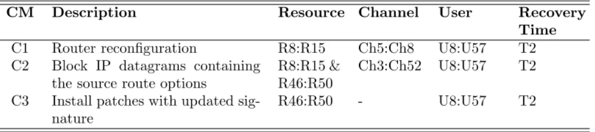
Three security countermeasures are proposed to mitigate attack A1. The input information of each security countermeasure is shown in Table 6. For instance, C1 proposes router reconfiguration, which should be performed in a short time (T2), affecting eight resources (R8:R15), three channels (Ch5:Ch8), and 50 user accounts (U8:U57).
In order to compute the geometrical operations detailed in Section 5, we need to determine the contribution of each dimension in the reduction of the attack’s impact level. Table 7 summarizes
Table 6: Countermeasure Information
CM Description Resource Channel User Recovery
Time
C1 Router reconfiguration R8:R15 Ch5:Ch8 U8:U57 T2
C2 Block IP datagrams containing
the source route options
R8:R15 & R46:R50
Ch3:Ch52 U8:U57 T2
C3 Install patches with updated
sig-nature
R46:R50 - U8:U57 T2
The ‘&’ symbol denotes a conjunctive
this information. For instance, C1 has a contribution of 27 units in the resource dimension, 8 units in the channel dimension, 150 units in the user dimension and three units in the recovery time dimension.
Table 7: Dimension Contribution
CM Resource (L1) Channel (L2) User (L3) Recovery Time (L4)
C1 8×3 = 27 4×2=8 50×3=150 1×3=3
C2 (8×3)+(5×2)= 37 50×2=100 50×3=150 1×3=3
C3 5×2 = 10 - 50×3=150 1×3=3
From Table 7 we can see that C1 and C2 have information of four dimensions (i.e., resource, channel, user, and recovery time). However, C3 does not have information of the channel dimension, since its implementation does not directly affect any of the system’ channels.
Using Equations 7, 14, 19, and 22, we calculate the perimeter, area, volume and hyper-volume of countermeasures C1 and C2 (4-orthotope) respectively. Geometrical measurements of countermea-sure C3 (cuboid) are performed using Equation 5 (Perimeter), Equation 12 (Area), and Equation 17 (Volume). The Hyper-volume of C3 is computed as the volume of the cuboid times one unit (empty axes are filled with one). Table 8 summarizes these results.
Table 8: Countermeasure Impact Measurement
CM Perimeter (P) Area (A) Volume (V) Hyper-Volume (H)
C1 752 units 6,021 units2 48,798 units3 97,200 units4
C2 1,160 units 25,111 units2 627,750 units3 166,500 units4
C3 652 units 1,980 units2 4,500 units3 4,500 units4
Figure 6 shows the graphical representation of countermeasures C1, C2, and C3 with respect to attack A1. This latter is represented as a cuboid with discontinuous line and grey color, whereas countermeasures C1, C2 and C3 are represented with colors red, blue and green respectively.
Resource 2040 6080100 120140 160180 200 0 100 200Channel300 400 500 User Account 0 50 100 150 200 250 300 350 A1 A1 A1 A1 A1 A1 A1 A1 A1 A1 A1 A1 C1 C2 C2 C3 A1:Attack C1:Router Reconfiguration C2:Block IP C3:Patches
(a) Resource - Channel - User
Resource 20 40 60 80 100 120 140 160 180 200 User Account 0 50 100 150 200 250 300 350 Time 4.04.55.0 5.56.0 6.57.0 A1 A1 A1 A1 C1C2 C2 C3 A1:Attack C1:Router Reconfiguration C2:Block IP C3:Patches
(b) Resource - User - Time
Resource 20 40 60 80 100120 140160 180200 Channel 0 100 200 300 400 500 Time 4.0 4.5 5.0 5.5 6.0 6.5 7.0 A1 A1 A1 A1 A1 A1 C1 C2 C2 C3 A1:Attack C1:Router Reconfiguration C2:Block IP C3:Patches
(c) Resource - Channel - Time
Channel 0 100 200 300 400 500 User Account 0 50 100 150 200 250 300 350 Time 4.0 4.5 5.0 5.5 6.0 6.5 7.0 A1 A1 A1 A1 A1 A1 C1 C2 C3 A1:Attack C1:Router Reconfiguration C2:Block IP C3:Patches
(d) Resource - User - Time
Figure 6: Graphical representation of the impact of attack A1 and countermeasures C1, C2, and C3
We provide different views of the graphical representation of A1 and the countermeasures, by selecting three dimensions at a time. For instance, Figure 6(a) shows the graphical representation of attack A1 and all countermeasures based on the information about the affected resources, channels and users. Figure 6(b) includes the information of affected resources and users vs. the recovery time. Figure 6(c) depicts the graphical representation of the affected resources and channels, vs. the recovery time. Figure 6(d) shows the graphical representation of the affected channels and users, vs. the recovery time.
7.4. Discussion
Considering that the graphical representation of instances in more than three dimensions results into complex figures that only provides a general overview of the size and density of the represented event, we limit this representation using a coordinate system with up to three dimensions. However, the mathematical computation of hyper-volumes can go up to the nth dimension.
For the previous case study, we have the attack impact expressed in units5 (the hyper-volume
4-orthotope), whereas countermeasure C3 is expressed in units3 (the volume of a cuboid).
Coun-termeasures are not analyzed using the location context, since this is an information that only concerns to the attack. Countermeasures are implemented locally, therefore there is no need to consider this dimension in the impact calculation.
To compare the magnitude of each event, we need to select a fixed dimensional space and make conversions, so that all events are expressed using the same notation. We can, for instance, decide to analyze events in five dimensions, which will require to add one or two more dimensions (with a value of one) to the countermeasure impact calculation. In such a case, all attacks and
countermeasures will be expressed in units5
For simplicity, we decided to work in a three dimensional space. For this, we need to compare
the volume (units3) of all events. Considering that the volume of attack A1 is 606,990 units3, we
refer to Table 8 to compare it with the volume of all countermeasures. As a result, C1 measures
48,798 units3 (more than ten times smaller than attack A1), C2 measures 627,750 units3 (bigger
than attack A1), and C3 measures 4,500 units3 (more than 100 times smaller than attack A1).
It is possible to have countermeasure volumes higher than the attack volume, since the attack compromises a portion of the system that is not necessarily covered in total by a single counter-measure. In this case, C2 affects elements that are not under attack, that can be considered as a
potential collateral damage7. The fact that C2 is bigger than attack A1 does not imply that the
attack is totally covered by the countermeasure. There is a set of channels and users that are not
treated by any countermeasure, which is therefore considered as a residual risk8.
8. Related Work
In this paper we introduced a geometrical model to measure the impact of events against critical infrastructures, as an improvement of the attack surface model. This latter has been initially proposed by Howard et al. [24, 25] as the union of code, interfaces, services, protocols, and practices available to users. The approach does not provide a systematic method to assign weights to the attack vectors; it focuses on measuring the attack surfaces of operating systems; and it is not possible to determine if all attack vectors have been identified.
In addition, Manadhata et al. [22, 21, 23] has been, so far, the only approach to systematically measure the attack surface of different software. The methodology cannot be applied in the absence of source code; it only compares the level of attackability between two similar systems; and it does not allow the security administrator to evaluate the impact of multiple attacks occurring simultaneously in a given system.
More recently, Kordy et al. [37, 38, 39] propose a framework that integrates graphical security modeling techniques of attackdefense trees with probabilistic information which allows to provide an intuitive and visually appealing representation of interactions between an attacker and a defender of a system. Authors state that there still a gap between theoretical research and practical employment of graphical security models.
We had initially proposed the attack volume model [11, 40] as an approach to measure the impact of complex attacks in a three dimensional coordinate system. The effectiveness of the approach is low for cases inr which the information of events is very limited (e.g., one or two dimensions),
7The damage to things that are incidental to the intended target. 8The risk that remains after the controls are taken into account.