HAL Id: hal-03103006
https://hal.archives-ouvertes.fr/hal-03103006
Submitted on 11 Jan 2021
HAL is a multi-disciplinary open access
archive for the deposit and dissemination of
sci-entific research documents, whether they are
pub-lished or not. The documents may come from
teaching and research institutions in France or
abroad, or from public or private research centers.
L’archive ouverte pluridisciplinaire HAL, est
destinée au dépôt et à la diffusion de documents
scientifiques de niveau recherche, publiés ou non,
émanant des établissements d’enseignement et de
recherche français ou étrangers, des laboratoires
publics ou privés.
scales over the last 2000 years
Barbara Stenni, Mark Curran, Nerilie Abram, Anais Orsi, Sentia Goursaud,
Valerie Masson-Delmotte, Raphael Neukom, Hugues Goosse, Dmitry Divine,
Tas van Ommen, et al.
To cite this version:
Barbara Stenni, Mark Curran, Nerilie Abram, Anais Orsi, Sentia Goursaud, et al.. Antarctic climate
variability on regional and continental scales over the last 2000 years. Climate of the Past, European
Geosciences Union (EGU), 2017, 13 (11), pp.1609-1634. �10.5194/CP-13-1609-2017�. �hal-03103006�
https://doi.org/10.5194/cp-13-1609-2017 © Author(s) 2017. This work is distributed under the Creative Commons Attribution 3.0 License.
Antarctic climate variability on regional and continental scales
over the last 2000 years
Barbara Stenni1,2, Mark A. J. Curran3,4, Nerilie J. Abram5,6, Anais Orsi7, Sentia Goursaud7,8,
Valerie Masson-Delmotte7, Raphael Neukom9, Hugues Goosse10, Dmitry Divine11,12, Tas van Ommen3,4, Eric J. Steig13, Daniel A. Dixon14, Elizabeth R. Thomas15, Nancy A. N. Bertler16,17, Elisabeth Isaksson11, Alexey Ekaykin18,19, Martin Werner20, and Massimo Frezzotti21
1Department of Environmental Sciences, Informatics and Statistics, Ca’ Foscari University of Venice, Venice, Italy 2Institute for the Dynamics of Environmental Processes, CNR, Venice, Italy
3Australian Antarctic Division, 203 Channel Highway, Kingston, Tasmania 7050, Australia
4Antarctic Climate & Ecosystems Cooperative Research Centre, University of Tasmania, Hobart 7001, Australia 5Research School of Earth Sciences, Australian National University, Canberra ACT 2601, Australia
6ARC Centre of Excellence for Climate System Science, Australian National University, Canberra ACT 2601, Australia 7Laboratoire des Sciences du Climat et de l’Environnement (IPSL/CEA-CNRS-UVSQ UMR 8212), CEA Saclay,
91191 Gif-sur-Yvette CEDEX, France
8Université Grenoble Alpes, Laboratoire de Glaciologie et Géophysique de l’Environnement (LGGE),
38041 Grenoble, France
9University of Bern, Oeschger Centre for Climate Change Research & Institute of Geography, 3012 Bern, Switzerland 10Université catholique de Louvain, Earth and Life Institute, Centre de recherches sur la terre et le climat Georges Lemaître,
1348 Louvain-la-Neuve, Belgium
11Norwegian Polar Institute, Fram Centre, 9296 Tromsø, Norway
12Department of Mathematics and Statistics, Faculty of Science, University of Tromsø – The Arctic University of Norway,
9037, Tromsø, Norway
13Department of Earth and Space Sciences, University of Washington, Seattle, WA 98195, USA 14Climate Change Institute, University of Maine, Orono, ME 04469, USA
15British Antarctic Survey, Cambridge, CB3 0ET, UK
16Antarctic Research Centre, Victoria University of Wellington, Wellington 6012, New Zealand 17National Ice Core Research Facility, GNS Science, Gracefield 5040, New Zealand
18Arctic and Antarctic Research Institute, St. Petersburg, Russia
19Institute of Earth Sciences, Saint Petersburg State University, St. Petersburg, Russia
20Alfred Wegener Institute, Helmholtz Centre for Polar and Marine Research, 27570 Bremerhaven, Germany 21ENEA Casaccia, Rome, Italy
Correspondence to:Barbara Stenni (barbara.stenni@unive.it) Received: 28 February 2017 – Discussion started: 22 March 2017
Abstract. Climate trends in the Antarctic region remain poorly characterized, owing to the brevity and scarcity of direct climate observations and the large magnitude of in-terannual to decadal-scale climate variability. Here, within the framework of the PAGES Antarctica2k working group, we build an enlarged database of ice core water stable iso-tope records from Antarctica, consisting of 112 records. We produce both unweighted and weighted isotopic (δ18O) com-posites and temperature reconstructions since 0 CE, binned at 5- and 10-year resolution, for seven climatically distinct regions covering the Antarctic continent. Following earlier work of the Antarctica2k working group, we also produce composites and reconstructions for the broader regions of East Antarctica, West Antarctica and the whole continent. We use three methods for our temperature reconstructions: (i) a temperature scaling based on the δ18O–temperature re-lationship output from an ECHAM5-wiso model simulation nudged to ERA-Interim atmospheric reanalyses from 1979 to 2013, and adjusted for the West Antarctic Ice Sheet re-gion to borehole temperature data, (ii) a temperature scaling of the isotopic normalized anomalies to the variance of the regional reanalysis temperature and (iii) a composite-plus-scaling approach used in a previous continent-scale recon-struction of Antarctic temperature since 1 CE but applied to the new Antarctic ice core database. Our new reconstruc-tions confirm a significant cooling trend from 0 to 1900 CE across all Antarctic regions where records extend back into the 1st millennium, with the exception of the Wilkes Land coast and Weddell Sea coast regions. Within this long-term cooling trend from 0 to 1900 CE, we find that the warmest period occurs between 300 and 1000 CE, and the coldest in-terval occurs from 1200 to 1900 CE. Since 1900 CE, signif-icant warming trends are identified for the West Antarctic Ice Sheet, the Dronning Maud Land coast and the Antarc-tic Peninsula regions, and these trends are robust across the distribution of records that contribute to the unweighted iso-topic composites and also significant in the weighted tem-perature reconstructions. Only for the Antarctic Peninsula is this most recent century-scale trend unusual in the con-text of natural variability over the last 2000 years. How-ever, projected warming of the Antarctic continent during the 21st century may soon see significant and unusual warm-ing develop across other parts of the Antarctic continent. The extended Antarctica2k ice core isotope database developed by this working group opens up many avenues for devel-oping a deeper understanding of the response of Antarctic climate to natural and anthropogenic climate forcings. The first long-term quantification of regional climate in Antarc-tica presented herein is a basis for data–model comparison and assessments of past, present and future driving factors of Antarctic climate.
1 Introduction
Antarctica is the region of the world where instrumental cli-mate records are shortest and sparsest. Esticli-mates of tempera-ture change with reasonable coverage across the full Antarc-tic continent are only available since 1958 CE (Nicolas and Bromwich, 2014), and the large magnitude of year-to-year climate variability that characterizes Antarctica makes the interpretation of trends in this data-sparse region problem-atic (Jones et al., 2016). As a result, the knowledge of past Antarctic temperature and climate variability is predomi-nantly dependent on proxy records from natural archives. While coastal proxy records are being developed from terres-trial and marine archives, information on Antarctic climate above the ice sheet exclusively relies on the climatic inter-pretation of ice core records.
Within the variety of measurements performed in bore-holes and ice cores, only water stable isotopes can provide subdecadal-resolution records of past temperature changes (Küttel et al., 2012). In high-accumulation areas of coastal zones and West Antarctica, annual layer counting is feasible during the last centuries to millennia (Plummer et al., 2012; Abram et al., 2013; Thomas et al., 2013; Sigl et al., 2016; Winstrup et al., 2017, under review), and annual water stable isotope signals can be delivered. However, in the dry regions of the central Antarctic plateau, where the longest ice core records are available, chronologies are less accurate and rely on the identification of volcanic deposits that can be used to tie ice cores from different sites to a common Antarctic ice core age scale (Sigl et al., 2014, 2015).
The chemical and physical signals measured in an individ-ual ice core reflect a local climatic signal archived through the deposition and reworking of snow layers. The intermit-tency of Antarctic precipitation (Masson-Delmotte et al., 2011; Sime et al., 2009), variability in precipitation source regions (Sodemann and Stohl, 2009), and post-depositional effects of snow layers including wind drift and scouring, sub-limation, and snow metamorphism (Frezzotti et al., 2007; Ekaykin et al., 2014; Touzeau et al., 2016; Casado et al., 2016; Hoshina et al., 2014; Steen-Larsen et al., 2014) can distort the climate signal preserved within ice cores and pro-duces non-climatic noise. As a result, obtaining a robust cli-mate signal can only be achieved through the combination of multiple ice core records from a given site and/or region, and through the site-specific calibration of the relationships between water stable isotopes and temperature.
Water can be characterized by the stable isotope ratios of oxygen (δ18O: the deviation of the ratio of18O/16O in a sam-ple, relative to that of the standard, Vienna Standard Mean Ocean Water) and of hydrogen (δD: the deviation of the ra-tio of2H/1H). Both of these parameters within ice cores pro-vide information on past temperatures. There is solid theo-retical understanding of distillation processes relating mois-ture transport towards the polar regions with air mass cool-ing and the progressive loss of heavy water molecules along
the condensation pathway (Jouzel and Merlivat, 1984). This theoretical understanding is further supported by numerical modelling performed using atmospheric general circulation models equipped with water stable isotopes (Jouzel, 2014). The effects of these processes are observed in the spatial relationships between the isotopic composition of Antarctic precipitation and surface snow and surface air temperature across the continent. However, relationships between water stable isotopes in snow and surface temperature may vary through time as a result of changes between condensation and surface temperature (in relation to changes in boundary layer stability), changes in moisture origin and initial evap-oration conditions, changes in atmospheric transport path-ways, and changes in precipitation seasonality or intermit-tency (Masson-Delmotte et al., 2008). Investigations based on the sampling of Antarctic precipitation have demonstrated that seasonal and inter-annual isotope vs. temperature slopes are generally smaller than spatially derived relationships (van Ommen and Morgan, 1997; Schneider et al., 2005; Stenni et al., 2016; Schlosser et al., 2004; Ekaykin et al., 2004; Fer-nandoy et al., 2010). Moreover, emerging studies combin-ing the monitorcombin-ing of surface water vapour isotopic compo-sition with the isotopic compocompo-sition retained in surface snow and precipitation have revealed that snow–air isotopic ex-changes during snow metamorphism affect surface snow iso-topic composition (Ritter et al., 2016; Casado et al., 2016; Touzeau et al., 2016). It is not yet possible to assess the im-portance of such post-deposition processes for the interpre-tation of ice core water stable isotope records, but they may enhance the relationship between snow isotopic composition and surface temperature more than expected from the inter-mittency of snowfall (Touzeau et al., 2016). Changes in ice sheet height due to ice dynamics may also affect the surface climate trends inferred from water stable isotope records; however, this influence should be of second order over the last 2000 year interval that is the focus of this study (Fe-gyveresi et al., 2011).
As a result, the two key challenges to reconstruct past changes in Antarctic temperature from ice core isotope records are (1) to develop methodologies to combine differ-ent individual or stacked ice core records in order to deliver regional-scale climate signals and (2) to quantify the temper-ature changes represented by water stable isotope variations. Goosse et al. (2012) first calculated a composite of Antarc-tic temperature simply by averaging seven standardized tem-perature records inferred from water stable isotopes using a spatial isotope–temperature relationship for the last mil-lennium. The first coordinated effort to reconstruct Antarc-tic temperature during the last 2000 years (PAGES 2k Con-sortium, 2013) screened published ice core records for an-nual layer counting or alignment of volcanic sulfate records and overlap with instrumental temperature data (Steig et al., 2009), leading to the selection of 11 records. The recon-struction procedure used a composite-plus-scaling (CPS) ap-proach similar to the methodology of Schneider et al. (2006)
and produced reconstructions of the continent-wide temper-ature history as well as specific West Antarctica and East Antarctica reconstructions. The skill of the reconstructions was limited by the number of available records through time (for instance, only one predictor in each region prior to 166 CE). This analysis identified significant (p < 0.01) cool-ing trends from 166 to 1900 CE, 2.5 times larger in West Antarctica than in East Antarctica. A robust cooling trend over this time period has also been identified from terrestrial and marine reconstructions from other regions (PAGES 2k Consortium, 2013; McGregor et al., 2015).
The comparison of these first Antarctic 2k time series with those from other regions obtained within the PAGES 2k working groups identified three specificities: (i) recon-structed Antarctic centennial variations did not correlate with those from other regions, (ii) the Antarctic region was the only one where a protracted cold period did not start around 1580 CE (iii) the Antarctic region was the only one where the 20th century was not the warmest century of the last 2000 years. A recent effort to characterize Antarctic and sub-Antarctic climate variability during the last 200 years also concluded that most of the trends observed since satellite climate monitoring began in 1979 CE cannot yet be distin-guished from natural (unforced) climate variability (Jones et al., 2016), and observed instrumental climate trends are of the opposite sign to those produced by most forced cli-mate model simulations over the same post-1979 CE inter-val. The only exception to this conclusion was for changes in the Southern Annular Mode (SAM), the leading mode of atmospheric circulation variability in the high latitudes of the Southern Hemisphere (SH), which has showed a significant and unusual positive trend since 1979 CE.
While changes in the SAM have been related to the hu-man influence on stratospheric ozone and greenhouse gases (Thompson et al., 2011), major gaps remain in identifying the drivers of multi-centennial Antarctic climate variability. For instance, the influence of solar and volcanic forcing on Antarctic climate variability remains unclear. This is due to both the lack of observations and to the lack of confi-dence in climate model skill for the Antarctic region (Flato et al., 2013). Goosse et al. (2012) have used simulations from an intermediate complexity model to attribute the Antarc-tic annual mean cooling trend from 850 to 1850 CE to vol-canic forcing. Recent comparisons of climate model simula-tions with the PAGES 2k regional reconstrucsimula-tions have high-lighted greater model–data disagreement in the SH than in the Northern Hemisphere (PAGES 2k–PMIP3 group, 2015; Abram et al., 2016); such disagreement could be due ei-ther to model deficiencies or to large uncertainties in the re-constructions, which were built on relatively small number of records. Changes in ocean heat content and ocean heat transport have likely contributed to the different temperature evolution at high southern latitudes compared to other re-gions of the Earth (Goosse, 2017), and model-based stud-ies have suggested that circulation in the Southern Ocean
may act to delay, by centuries, the development of sustained warming trends in high southern latitudes (Armour et al., 2016). Antarctic temperature reconstructions spanning the last 2000 years may help to better constrain the processes and timescales by which natural and anthropogenic forcing act to affect climate changes in the Antarctic region.
This motivates our efforts to produce updated Antarc-tic temperature reconstructions. The previous continent-scale reconstruction (PAGES 2k Consortium, 2013), in which only a limited number of records have been used, may mask im-portant regional-scale features of Antarctica’s climate evo-lution. Here we use an expanded paleoclimate database of Antarctic ice core isotope records and new reconstruc-tion methodologies to reconstruct the climate of the past 2000 years, on a decadal scale and regional basis. Seven distinct climatic regions have been selected: the Antarctic Peninsula, the West Antarctic Ice Sheet (WAIS), the East Antarctic Plateau and four coastal domains of East Antarc-tica. This regional selection, which is supported by regional atmospheric RACMO2.3p2 model results (Thomas et al., 2017; Van Wessem et al., 2014), is applied to both Antarc-tic ice-core-derived isotopic (temperature proxy) and snow accumulation rate reconstructions (see companion paper in the same issue by Thomas et al.). Section 2 describes the ice core and the temperature data sets used in this study, as well as the modelling framework used to support the anal-ysis. The climate region definition, the preprocessing of the data and the different reconstruction methods are presented in Sect. 3. Section 4 discusses our new regional isotopic and temperature reconstructions for Antarctica, including the ap-plication of the previous methodology to the new database. Finally, Sect. 5 presents the summary of our results and their implications.
2 Data sets
2.1 Ice core records
Here we present and use a new expanded database that has been compiled in the framework of the PAGES Antarc-tica2k working group. The initial selection criteria are those requested by the PAGES 2k network (http://www. pages-igbp.org/ini/wg/2k-network/data) for the building of the community-sourced database of temperature-sensitive proxy records (PAGES 2k Consortium, 2017). Briefly, (i) the records must be publicly available and published, (ii) a re-lation between the climate proxies and variables should be stated, (iii) the record duration should be between 300 and 2000 years, (iv) the chronology, certified by the data owner, should contain at least one chronological control point near the end (most recent) part of the record and another near the oldest part of the record and (v) the resolution should be at least one analysis every 50 years.
In building the Antarctica2k database we also allow shorter records to be included, although we request a
strati-graphic control using volcanic markers (Sigl et al., 2014) and, whenever possible, a dating by annual layer counted chronology. This last requirement is only possible in the high-accumulation regions of West Antarctica, the Antarctic Peninsula and coastal areas of East Antarctica. The inclusion of shorter records is designed to improve data coverage for assessments of climatic trends in Antarctica during the past century. The 11 records included in the previous continent-scale reconstruction (PAGES 2k Consortium, 2013) relied on a highly precise chronological framework consisting of a common chronology, which used 42 volcanic events to synchronize the records. Here, we use both high- and low-resolution records. Most of the records have a data low-resolution ranging from 0.025 to 5 years (only three records have a reso-lution of > 10 years). Previous studies (Frezzotti et al., 2007; Ekaykin et al., 2014) have shown that post-depositional and wind scouring effects, acting more effectively when the ac-cumulation rate is very low, limit our ability to obtain tem-perature reconstructions at annual resolution in most of the interior of Antarctica. Because of this, in our regional recon-structions we use 5-year-averaged data for reconstructing the last 200 years, and 10-year averages for reconstructing the last 2000 years. Using 5- or 10-year averages also decreases our dependence on an annually precise chronological straint between the ice core records, allowing us to more con-fidently use the expanded database. The data have been also screened for glaciological problems, with those records that are very likely to be affected by ice flow dynamics excluded. This enlarged database consists of 112 isotopic records. A list of the records used are reported in Table S1 (in the Supplement) and their spatial distribution is shown in Fig. 1. Figure S1 shows the location of the ice core sites along with a visualization of the record lengths. Most of the records of this new database cover the last 200 years and this is particu-larly true for the more coastal areas. Within the database, 36 records cover just the last 50 years or less, while 50 records cover the whole length of the past 200 years. There are 15 records that cover the last 1000 years, while only nine records reach as far back as 0 CE.
2.2 Temperature product
The instrumental record is very short in Antarctica, and most ice core sites do not have weather station measurements asso-ciated with the cores. In addition, the retrieval of the first me-tre of firn can be difficult, due to poor cohesion of the snow. As a result, for many sites, there is no overlap between in-strumental and proxy data, which complicates the proxy cal-ibration exercise. To enlarge the calcal-ibration data set, we use the climate field reconstruction from Nicolas and Bromwich (2014) (hereafter NB2014; http://polarmet.osu.edu/datasets/ Antarctic_recon/). This surface temperature data set provides homogeneous data at 60 km resolution, extends from 1957 to 2013 and includes the revised Byrd temperature record (Bromwich et al., 2013) that improves the skill of the
tem-Figure 1.(a) Schematic map of the seven Antarctic regions selected for the regional reconstructions. In blue is the East Antarctic Plateau, in light blue the Wilkes Land Coast, in green the Weddell Sea Coast, in yellow the Antarctic Peninsula, in orange the West Antarctic Ice Sheet, in red the Victoria Land Coast–Ross Sea and in brown the Dronning Maud Land Coast. The dots show the site locations. The white dots represent the sites that have been used in the previous continent-scale reconstruction (PAGES 2k Consortium, 2013). (b) Correlation maps between the regional mean temperature and each grid point using the Nicolas and Bromwich (2014) data set.
perature product over West Antarctica. It covers a longer time span than reliable atmospheric reanalysis products for Antarctica (which begin only in 1979 CE) and has a higher spatial resolution than available isotope-enabled general cir-culation model (GCM) outputs. This data set is used to es-timate the spatial representativeness of individual core sites (Sect. 3.3.2), to scale the normalized isotopic anomaly data to temperature (Sect. 3.4.2) and to calculate the surface tem-perature reconstructions with the CPS method (Sect. 3.4.4).
2.3 Modelling framework
In order to use model information on isotope–temperature relationships in Antarctic precipitation, we use a reference simulation performed using the general atmospheric circu-lation model ECHAM5-wiso. The initial ECHAM5 model (Roeckner et al., 2003) has been equipped with water sta-ble isotopes (Werner et al., 2011), following earlier work on ECHAM3 (Hoffmann et al., 1998) and ECHAM4 (Werner et al., 2001), and accounting for fractionation processes dur-ing phase changes. This model is used here because re-cent studies, based on model–data comparisons using ob-servations of precipitation and surface vapour isotopic com-position on a global scale and in the Arctic (e.g. Werner et al., 2011; Steen-Larsen et al., 2017) have shown strong model skill of ECHAM5-wiso when it is run in high reso-lution as in this study (T106, with a mean horizontal grid resolution of approximately 1.1◦×1.1◦). A study of the
2012 atmospheric river event in Greenland has demonstrated the skill of ECHAM5-wiso to reproduce these events, with a good representation of the water isotope signature (Bonne et al., 2014). In Antarctica, model performance was assessed against a compilation of surface data (Masson-Delmotte et al., 2008) and recent measurements of vapour and precipi-tation (Ritter et al., 2016; Dittmann et al., 2016).
Here, we use a 1958–2014 CE simulation in which ECHAM5-wiso was nudged to atmospheric reanalyses from ERA-40 (Uppala et al., 2005) and ERA-Interim (Dee et al., 2011) and run using the same ocean surface boundary con-ditions (sea surface temperature and sea ice) as in ERA-40 and ERA-Interim. Ocean surface water isotopic values were set to constant values using a compilation of observational data (Schmidt et al., 2007). Inter-comparisons of reanalysis products showed good skills of ERA-Interim for Antarctic precipitation (Wang et al., 2016), surface temperature, and vertical profiles of winds and temperatures. However, com-parisons with in situ observations reveal an underestimate of precipitation and a slight cold bias in the surface tempera-tures in some regions (Thomas and Bracegirdle, 2015).
The ECHAM5-wiso simulations produce a large increase, which is not observed in instrumental or ice core data, in the temperature and the δ18O outputs prior to 1979 (Goursaud et al., 2017). This arises from a discontinuity in the ERA-40 reanalyses due to the lack of observations available for assimilation and boundary conditions prior to the satellite era (e.g. Antarctic sea ice) (Nicholas and Bromwich, 2014). We
therefore use the ECHAM5-wiso simulations only for 1979– 2013 CE.
For the analysis of the isotope–temperature relationships at each individual ice core site, we extracted the grid point data closest to each site. For the analysis of isotope relation-ships on a regional scale, we calculated the area-weighted average of model outputs at grid points within the region. The δ18O–temperature relationship was calculated using the annual or seasonal average 2 m temperature and annual precipitation-weighted δ18O, to mimic deposition processes. The simulation does not account for post-deposition pro-cesses (i.e. diffusion, which is not important on the 5- and 10-year timescales considered here; e.g. Küttel et al., 2012).
3 Methodology
3.1 Defining climatic regions
Earlier work of the PAGES Antarctica2k working group pro-duced a continent-scale temperature reconstruction for the whole of Antarctica, as well as reconstructions for East and West Antarctica based on a separation approximated by the Transantarctic Mountains (PAGES 2k Consortium, 2013). These broad-scale groupings mask important regional cli-matic trends noted in individual studies. In particular, the absence of recent significant warming in the Antarctica2k continent-scale temperature reconstruction is known to not be representative of all Antarctic locations (e.g. Steig et al., 2009, 2013; Mulvaney et al., 2012; Abram et al., 2013).
In this study, we choose seven climatic reconstruction re-gions (Fig. 1). These rere-gions are defined based on our knowl-edge of regional climate and snow deposition processes in the Antarctic region, as well as the availability of ice core isotope records. In particular, we separated coastal regions (below 2000 m altitude) from the East Antarctic Plateau: coastal sites receive moisture from the high-latitude Southern Ocean and are affected by the nearby sea ice cover (Masson-Delmotte et al., 2008). In contrast, high-altitude sites receive moisture that has travelled at higher altitude, originating from further afield, and from clear sky precipitation (Ekaykin et al., 2004). The regional selections were further validated and refined by spatial correlation of temperature using the NB2014 data product. The seven climatic regions are defined as follows (see Table S1):
1. For East Antarctic Plateau, all East Antarctic contiguous regions are at an elevation higher than 2000 m, includ-ing everythinclud-ing south of 85◦S. We exclude high peaks of the Transantarctic Mountains if they belong to the Vic-toria Land–Ross Sea coast (e.g. Taylor Dome or Her-cules Névé).
2. Wilkes Land Coast sits at an altitude < 2000 m and ex-tends from Lambert Glacier (67◦E) east to the start of Victoria Land and the Transantarctic Mountains (160◦E).
3. Weddell Sea Coast extends eastward from longitude 60 to 30◦W, and south of 75◦S, and lies at an altitude
<2000 m. Eastward of the 30◦W longitude, the 75◦S
latitude defines the boundary with the Dronning Maud Land coast region, with the northeastern corner of the Weddell Sea Coast region occurring where the 75◦S lat-itude meets the 2000 m elevation contour. This region includes the Filchner Ice Shelf and most of the Ronne Ice Shelf.
4. Antarctic Peninsula encompasses the mountainous Antarctic Peninsula. Between 74 and 70◦S the longitu-dinal boundaries lie between 60 and 80◦W, while north
of 70◦S the longitudinal boundaries increase to 50–
80◦W so as to capture the northern end of the peninsula. 5. West Antarctic Ice Sheet is bounded by longitudes 60 to 170◦W, and north of 85◦S. In the Antarctic Peninsula region (60–80◦W) a northern bound of 74◦S is also ap-plied.
6. Victoria Land Coast–Ross Sea is north of 85◦S and at an altitude < 2000 m, with the exception of some local-ized peaks within the Transantarctic Mountains. It ex-tends from 160 to 190◦E (i.e. 170◦W) and incorporates most of the Ross Ice Shelf.
7. Dronning Maud Land Coast extends eastward from 30◦W to 67◦E (Lambert Glacier). The southernmost
boundary lies at 75◦S (where this region borders with
the Weddell Sea Coast region), or at the 2000 m eleva-tion contour elsewhere.
In addition to these seven climatic regions, we also produce reconstructions for a continent-wide Antarctic region. Broad-scale East Antarctic (incorporating the climatic regions of the East Antarctic Plateau, as well as the Weddell Sea, Dronning Maud Land, Wilkes Land and Victoria Land coasts) and West Antarctic (incorporating the climatic regions of the West Antarctic Ice Sheet and Antarctic Peninsula) reconstructions are also presented. These additional reconstructions facili-tate comparisons of our new results, using additional meth-ods and an expanded database, with earlier findings of the Antarctica2k working group and subsequent research using the 2013 continent-scale reconstruction for Antarctic temper-ature.
3.2 Data preprocessing
All ice core records in the Antarctica2k database were as-signed to one of the climatic regions described in Sect. 3.1 (as well as to East vs. West Antarctica and to the Antarctic-wide classifications). The majority (94 out of 112) of ice core water isotope records in the database are based on oxygen isotope ratios (δ18O). In cases in which only deuterium iso-tope (δD) data are available, the ice core time series were converted to an δ18O equivalent by dividing by 8, a value
that represents the slope of the global mean meteoric rela-tionship of oxygen and deuterium isotopes in precipitation and is close to the ratio of 7.75 observed in surface Antarctic snow (Masson-Delmotte et al., 2008).
The ice core δ18O (and δ18O equivalent) records were compiled on a common annual average age scale. For records with sub-annual resolution this involved averaging all data from within a calendar year to generate an annual average data set. Pseudo-annual records were generated for the ice core δ18O records with lower-than-annual resolution. These pseudo annuals assume that each low-resolution isotopic value represents an average of the full-time interval that the sample covers. As such, a nearest-neighbour interpolation method was used to generate stepped (piecewise constant) pseudo-annual records that continue the measured isotopic value across all of the calendar years that it represents.
Records were next binned to 5- and 10-year-average res-olution and converted to δ18O anomalies. This reduction in resolution is designed to reduce the influence of small age un-certainties between the records, as well as the non-climatic noise induced by post-deposition (e.g. wind erosion, diffu-sion) processes (Frezzotti et al., 2007; Ekaykin et al., 2014). The 5-year resolution records were converted to anomalies relative to their mean over the 1960–1990 CE interval, and records that do not include a minimum of six bins (30 years) of coverage since 1800 CE are excluded based on length. Overall, 79 records in the new Antarctica2k water isotope database meet the minimum requirement of having at least 30 years of data coverage since 1800 CE. In some cases, records meet this minimum length requirement but do not in-clude data for the full 1960–1990 CE reference interval. We adjust the mean value of each of these records by match-ing the mean δ18O of their most recent six bins (30 years) of data to the mean of all anomaly records from the same climatic region and over the same six-bin interval. We also produce normalized records by adjusting the variance in the records using the same reference period and method as for the anomaly records.
The 10-year resolution anomaly and normalized records were generated using the same method but using a reference period of 1900–1990 CE and a minimum data coverage of nine bins (90 years) since 0 CE. Similarly, records that do not include the full 1900–1990 CE reference period have the mean of their most recent nine-bin (90 years) interval ad-justed to match the mean of all other anomaly records from the same region and over the same nine-bin interval. Overall, 67 records in the new Antarctica2k water isotope database meet the minimum requirement of having at least 90 years of data coverage since 0 CE.
Some regions of Antarctica, such as coastal and plateau sites in Dronning Maud Land, include dense networks of ice core data (Fig. S1). To reduce possible bias towards these data-rich regions, an additional data reduction method was used based on a 2◦ latitude by 10◦ longitude grid. Where multiple ice core records from the same climatic region fall
within the same grid cell, their isotopic anomalies (or nor-malized data) are averaged to produce a single composite time series for the grid. This replicates the simple unweighted compositing method described in Sect. 3.3.1, but on the grid scale to reduce the representation of data-rich areas prior to the regional compositing. Figures S2 and S3 show the distri-bution of records by region that meet the six-bin (30 years) and nine-bin (90 years) minimum requirements for the 5- and 10-year composites, respectively, after the gridded data re-duction step.
3.3 Compositing methods
We use a suite of reconstruction methods of varying com-plexity in order to assess robust trends and variability in Antarctic ice core δ18O records and temperature.
3.3.1 Unweighted composites
Our first reconstruction method involves calculating simple composites of δ18O anomalies. For each 5- or 10-year bin we calculate the mean δ18O anomaly across all records in the climatic region, as well as the distribution of δ18O anoma-lies within each bin (Figs. 2 and 3). This basic reconstruc-tion method is analogous to that used for the Ocean2k low-resolution reconstruction (McGregor et al., 2015). The ben-efit of this simple method is that it requires no weighting or calibration assumptions, which is advantageous for data-sparse regions such as Antarctica (and the global oceans). The disadvantage is that it applies equal weighting to all records within a climatic region, which may introduce biases related to record length, location and climatic skill.
3.3.2 Weighted composites based on site-level temperature regressions
In order to avoid biases from uneven data sampling, we per-formed, for each region, a multiple regression between each site temperature and the relevant regional average temper-ature (Figs. 2 and 3). Most of the ice core records do not cover the full instrumental period; thus, it is problematic to use the δ18O anomalies directly to determine the regression vectors required for a weighted temperature reconstruction. Instead, we use the climate field reconstruction of NB2014 to estimate the weights: the annual mean temperature time series at the grid cell corresponding to each ice core site is extracted from the NB2014 product, and the regional average is also calculated for each reconstruction region. Regression-based weightings are calculated Regression-based on the relationship be-tween site temperature and regional average temperature, and the regression is performed for each combination of ice core records through time. The weights are then applied to the ice core δ18O anomalies to produce regional, averaged, standard-ized anomalies.
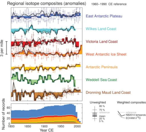
Figure 2.Regional δ18O composite reconstructions over the last 200 years using 5-year-binned anomaly data. Both unweighted composites and weighted composites (using both NB2014 temperature and ECHAM δ18O weighting methods) are shown. For each 5-year bin of the unweighted data, the mean δ18O anomaly across all records in the climatic region, as well as the distribution of δ18O anomalies within each bin, is calculated. All anomalies are expressed relative to the 1960–1990 CE interval. The number of records that contribute to the reconstructions for each region are displayed in the lower panel.
We further reproduced this regression method using both the δ18O and temperature field outputs from the ECHAM5-wiso experiments. The regression of site δ18O compared to regional average δ18O, or site temperature onto regional temperature, gave nearly identical weighting factors, sup-porting the use of the temperature field to calculate re-gressions. The effects of the different weighting methods on each regional isotopic composite, as well as the ini-tial 10-year isotopic anomaly records, are reported in the Supplement (Figs. S4–S10). The small differences between ECHAM- and NB2014-based regressions were due to the lower resolution of ECHAM5-wiso, which does not include islands and topographic features such as Roosevelt Island and Law Dome. For this reason, we preferentially use the NB2014 data set for the temperature regression reconstruc-tion method.
3.4 Temperature reconstructions
The relationship between δ18O and local surface tempera-ture is complicated by the influence of a large range of pro-cesses (origin of moisture sources, intermittency in
precipita-tion, snow drift, snow–air exchanges, snow metamorphism, diffusion in ice cores). It is not possible to consider each pro-cess independently because in many cases there are simply no observations to constrain them well enough. However, the atmospheric circulation often leads to several processes to be correlated (reduced sea ice, increased precipitation and warmer temperature, for instance). Here, we follow the clas-sical approach, which is to perform a linear regression of ice core δ18O with local surface temperature on the regional av-erage products. This method has the advantage of looking at all the climatic processes influencing δ18O in “bulk”, and the use of regional average allows us to limit the influence of small-scale processes.
The lack of an overlap period between our site δ18O records and direct temperature observations makes the proxy calibration difficult. The CPS method (Sect. 3.4.4), which replicates the 2013 PAGES 2k reconstruction method, is lim-ited to sites where this calibration is possible. To overcome this limitation and include the largest number of records, we also use models to scale the regional isotope compos-ites. A first method uses ECHAM5-wiso to determine the re-gional δ18O–temperature relationship in a mechanistic way
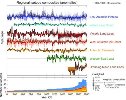
Figure 3.Regional δ18O composite reconstructions over the last 2000 years using 10-year-binned anomaly data. Both unweighted compos-ites and weighted composcompos-ites (using both NB2014 temperature and ECHAM δ18O weighting methods) are shown. For each 10-year bin of the unweighted data, the mean δ18O anomaly across all records in the climatic region, as well as the distribution of δ18O anomalies within each bin, is calculated. All anomalies are expressed relative to the 1900–1990 CE interval. The number of records that contribute to the reconstructions for each region are displayed in the lower panel.
(Sect. 3.4.1). A second method uses a more statistical ap-proach and simply scales the normalized record to the instru-mental period temperature variance (Sect. 3.4.2). Both ap-proaches are equally valid and share the same hypothesis: that the instrumental period (1979–2013) is representative of the longer-term climate variability. Finally, for the West Antarctic Ice Sheet region, an independent longer-term tem-perature record is available from borehole temtem-perature mea-surements (Orsi et al., 2012). We use this independent tem-perature record to scale the long term 1000–1600 CE temper-ature trend for the West Antarctic Ice Sheet region to provide our best estimate of temperature change in line with current knowledge (Sect. 3.4.3).
In the figure captions, we refer to the different methods as “ECHAM”, “NB2014” and “borehole”, respectively.
3.4.1 Scaling using model-based regional δ18O–temperature relationships
We use the coherent physical framework of the 1979– 2013 CE simulation performed at T106 resolution with ECHAM5-wiso to infer constraints on regional δ18O– temperature slopes through linear regression analysis be-tween regional averages of simulated annual mean temper-ature and precipitation-weighted δ18O (Table 1). These re-gional δ18O–temperature regressions were applied to the
re-gional ice core composites (δ18Oregion anomalies) to scale
them from δ18O to temperature units (Figs. 4 and 5) and produce temperature anomalies (Tregion). The correlation
co-efficient αregion is calculated using the York et al. (2004)
method, taking into account uncertainties both in Tregionand
in δ18Oregion, with each prior uncertainty equal to 20 % of the
variance.
Tregion=αregionδ18Oregion=αregion
X
sites i
wiδ18Oi
In this equation, wi represents the weights assigned to each
site i, and δ18Oi the site δ18O anomalies in 5- or
10-year-averaged records. The limited length of the observational pe-riod (1979–2013 CE) does not allow us to precisely estimate the slope α on 10-year averages, and we preferred to use 1-year anomalies, for which the slopes are significant (Ta-ble 1), and apply these slopes to the 10-year-binned com-posites. This implies that the interannual δ18O–temperature relationship comes from mechanisms that are also applica-ble to decadal-scale variability. It is impossiapplica-ble to further test this hypothesis without longer independent temperature records. The use of the ECHAM5-wiso isotope-enabled cli-mate model is the most up-to-date tool we have to quantify the δ18O–temperature on broad spatial–temporal scales and is our best tool to infer the δ18O–temperature relationship in the absence of data. Its main limitation is the model
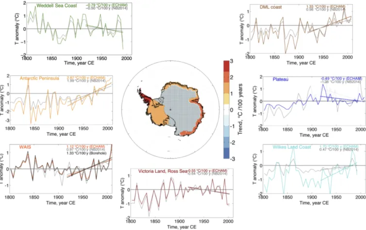
resolu-Figure 4.Regional temperature (T anomalies in◦C, referenced to the 1960–1990 CE interval) reconstructions using 5-year-binned data for the past 200 years. The weighing method is based on the correlation between site T and regional T from NB2014. The temperature scaling method is (i) based on the correlation between annual mean regional δ18O and regional T from ECHAM5-wiso forced by ERA-Interim (coloured lines) and (ii) scaled on the NB2014 target over 1960–1990 CE (grey lines), and the (iii) West Antarctic Ice Sheet region is adjusted to match the temperature trend between 1000 and 1600 CE based on borehole temperature measurements (black line; Orsi et al., 2012). Linear trends are calculated over the last 100 years of the reconstructions (colours match associated reconstruction methods). The map at the centre reports regional trends over the last 100-year trend using 5-year data based on the ECHAM method adjusted for the West Antarctic Ice Sheet region to borehole data. Hatched areas are not significant (p > 0.05).
Table 1.Linear regression analysis (slope with ±1σ uncertainty, correlation coefficient r, and p value) of the simulated δ18O–temperature relationships extracted from the ECHAM5-wiso model for each climatic region, as well as the broad East Antarctic, West Antarctic and whole of Antarctica regions.
Geographic region Slope (◦C ‰−1) Slope (‰◦C−1) r pvalue 1. East Antarctic Plateau 0.95 ± 0.05 1.05 ± 0.06 0.62 0.0001 2. Wilkes Land Coast 1.91 ± 0.11 0.52 ± 0.03 0.44 0.0084 3. Weddell Sea Coast 1.01 ± 0.06 0.99 ± 0.06 0.34 0.0449 4. Antarctic Peninsula 2.50 ± 0.15 0.40 ± 0.02 0.31 0.0658 5. West Antarctic Ice Sheet 1.04 ± 0.06 0.96 ± 0.05 0.59 0.0002 6. Victoria Land Coast 0.83 ± 0.05 1.21 ± 0.07 0.49 0.0027 7. Dronning Maud Land Coast 1.08 ± 0.06 0.93 ± 0.05 0.39 0.0217 West Antarctica 1.03 ± 0.06 0.97 ± 0.05 0.62 0.0001 East Antarctica 1.00 ± 0.05 1.00 ± 0.05 0.58 0.0002 All Antarctica 1.02 ± 0.06 0.98 ± 0.05 0.56 0.0004
tion: it is missing some coastal topographical features, no-tably James Ross Island, Roosevelt Island, and Law Dome,
and cannot faithfully represent regions where these sites are important.
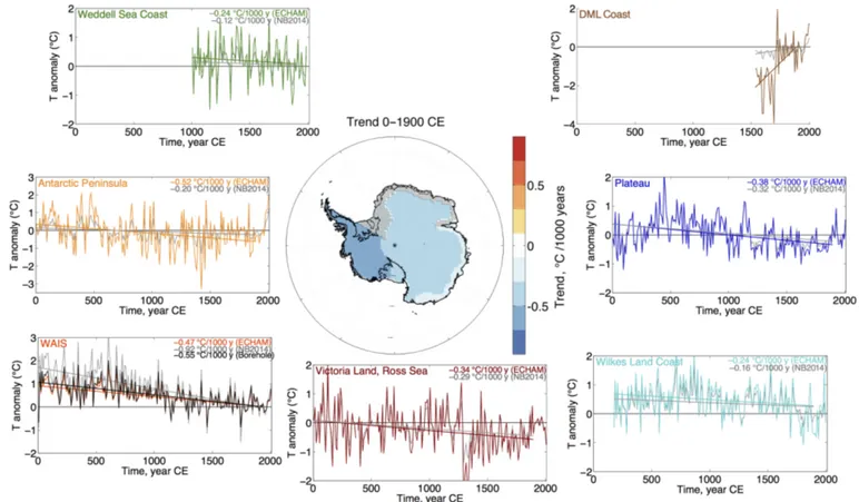
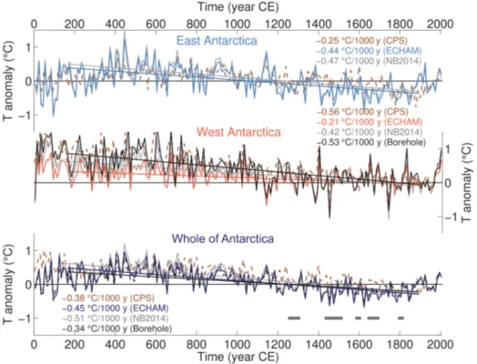
Figure 5.Regional temperature (T anomalies in◦C, referenced to the 1900–1990 CE period) reconstructions using 10-year data for the past 2000 years. Weighing method based on the correlation between site T and regional T from NB2014 forced by ERA-Interim. The temperature scaling method is (i) based on the correlation between annual mean regional δ18O and regional T from ECHAM5-wiso forced by ERA-Interim (coloured lines) and (ii) scaled on the NB2014 target over 1960–2010 CE (grey lines), and the (iii) West Antarctic Ice Sheet region is adjusted to match the temperature trend between 1000 and 1600 CE based on borehole temperature measurements (black line; Orsi et al., 2012). Linear trends are calculated over the period 0–1900 CE using 10-year-binned data. The map at the centre reports the trend values calculated between 0 and 1900 CE using 10-year data based on the ECHAM method adjusted to borehole data for the West Antarctic Ice Sheet region (the hatched area is not significant).
All regional δ18O–temperature relationships produced by the ECHAM5-wiso output are statistically significant (at 95 % confidence) with the exception of the Antarctic Penin-sula. Weak correlations are also found for the Weddell Sea Coast (r = 0.34). Stronger correlation coefficients are ob-tained inland, for the larger-scale East and West Antarctic sectors, and maximum values (r = 0.62) are identified for the East Antarctic Plateau.
Similarly, the simulated regional δ18O–temperature slopes are highest for Victoria Land (1.21 ‰◦C−1) and lowest for the Antarctic Peninsula (0.40 ‰◦C−1). This low slope for the Antarctic Peninsula does not agree with the temporal δ18O–temperature relationship that has been reported for the highly resolved James Ross Island ice core (0.86 ‰◦C−1; Abram et al., 2011), while it is similar to one reported for the Gomez ice core (0.5 ‰◦C−1; Thomas et al., 2009) and precipitation samples collected at the O’Higgins Sta-tion (0.41 ‰◦C−1; Fernandoy et al., 2012). ECHAM finds that the only site on the peninsula with a significant correla-tion between δ18O and temperature is Bruce Plateau (66◦S,
64◦W) (slope = 0.63 ± 0.58 ‰◦C−1, r = 0.13, p = 0.03), and the overall low δ18O–temperature slope is largely at-tributable to model resolution. We expect that the ECHAM scaling will produce a temperature reconstruction with a high-amplitude bias in the Antarctic Peninsula.
High slopes similar to the Victoria Land are identi-fied in the inland East Antarctic Plateau, Weddell Sea Coast and West Antarctic Ice Sheet regions (1.05, 0.99 and 0.96 ‰◦C−1, respectively), together with intermediate val-ues in coastal Dronning Maud Land with a 0.93 ‰◦C−1 mean slope. On the scale of the whole Antarctic ice sheet, the overall temporal slope is dominated by inland regions and simulated at 0.98 ‰◦C−1. This analysis is more thor-oughly examined in a study comparing an isotopic data set from surface snow, snowfalls and ice cores (Sentia Goursaud, personal communication, 2017).
3.4.2 Scaling based on NB2014 variance
In addition, we used an independent method of scaling the normalized δ18O anomalies to the SD (σ (T )) of the regional temperature from NB2014, over the 1960–1990 CE inter-val for the 5-year-binned averages, and the period 1960– 2010 CE for the 10-year-binned averages. This scaling is similar to the one used for the CPS method (see next sec-tion).
Tregion=σ(T )regionδ18Oregion(normalized)
This scaling method implies that the δ18O–temperature re-lationship can be inferred from the ratio of temperature to δ18O SD, which would be true if the relationship between the two were purely linear. If some of the δ18O variance is due to something other than temperature, this scaling will underestimate temperature variations. This method also as-sumes that the last 30 to 50 years provide a good estimate of the 5- or 10-year temperature variance. In the absence of longer temperature reconstructions, this is the best estimate of σ (T )regionthat we can provide.
3.4.3 Scaling based on borehole temperature for the WAIS region.
In the West Antarctic Ice Sheet region, the approaches de-scribed above give different results (Figs. 4 and 5), with the first method (temperature scaling from the δ18O–T re-lationship in ECHAM5-wiso) giving a smaller amplitude. At WAIS Divide, there is an independent temperature record, which can be used to scale the long-term temperature evo-lution. We used the borehole temperature reconstruction at WAIS Divide (Orsi et al., 2012) to adjust the amplitude of temperature variations, matching the cooling trend over the period 1000–1600 CE (−1.1◦C 1000 yr−1), with a correction factor relating the WAIS Divide site to the West Antarctic re-gion (c = σWAIS/σWDC=0.65), with σWAIS the SD of the
annual NB2014 WAIS regional mean data set, and σWDCthe
SD of the annual NB2014 time series at the WAIS Divide site, which gives a 1000–1600 CE cooling trend of −0.76◦C. This scaling is actually in line with the other two scalings: 1000–1600 CE slope of −0.65◦C for ECHAM and −1.01◦C for NB2014 scaling. The temperature calibration presented here is the best estimate we can provide with current knowl-edge, but we expect it to be revised in the future, with more precise δ18O modelling and more independent quantitative temperature reconstructions.
3.4.4 Replication of the 2013 Antarctica2k reconstruction method
To facilitate comparison with the preceding Antarctica2k temperature reconstruction published by the PAGES 2k Con-sortium (2013), we apply their reconstruction method to the
updated ice core isotope data collection. The method is a sim-ple CPS approach (Jones et al., 2009), updated from Schnei-der et al. (2006) and implemented similarly to Neukom et al. (2014). We apply this method to all subregions de-fined above, the broad East and West Antarctic divisions and to the Antarctic-wide database, replicating the Antarctic re-constructions presented in the PAGES 2k Consortium (2013) study.
First, the annual-average records are allocated to the cli-matic regions as defined above. The following steps are then repeated for each region separately. Second, only the records with no missing values in the 1961–1991 CE calibration pe-riod are selected. These records are then scaled to mean zero and unit SD over their common interval of data availability. Next, the normalized records are correlated with the NB2014 regional mean temperatures over 1961–1991 CE. Between 0 and 33 % of the ice core records within each region have neg-ative correlations (physically implausible) with the target and are removed from the proxy matrix. A composite of the re-maining records is then calculated by creating a weighted av-erage, where the weighting of each ice core record is based on its temperature correlation from the previous step. The composite is then scaled to the mean and SD of the NB2014 regional temperatures over the 1961–1991 CE period. The compositing and scaling steps are carried out with a nested approach, i.e. repeated for all periods with different proxy data availability.
In the reconstruction of the PAGES 2k Consortium (2013), three records were infilled with neighbouring sites to have no missing data in the calibration window: WDC06A was in-filled with data from WDC05A, and Siple Station and Plateau Remote records were infilled by a least median of squares multiple linear regression using nearby records (PAGES 2k Consortium, 2013). To allow comparison, we also used the infilled data for these records. Thus, the only difference from the reconstruction of PAGES 2k Consortium (2013) is that we use an extended proxy database with more records and an updated temperature target (NB2014 instead of Steig et al., 2009).
While this CPS approach allows a quantitative calibra-tion to the NB2014 temperature data, it has some limitacalibra-tions compared to the methods above. First, in this implementa-tion it allows only the inclusion of data covering the cali-bration period, thereby removing more than half of the avail-able records (62 out of 112). Second, the calibration period is extremely short and therefore individual years (for example with outliers) can significantly bias the reconstruction, and reasonable validation of the reconstruction is hardly possible. The main difference from the other compositing methods de-scribed above is the weight of each record and the interval over which the data are standardized.
4 Results and discussion
We use the varying reconstruction methods to identify robust trends in the Antarctic ice core database. We present results based on isotopic trends, as well as temperature reconstruc-tions, and examine these for the seven climatic regions and for the larger-scale Antarctic regions (Sect. 4.1), compare our results to the previous Antarctic temperature reconstruction (Sect. 4.2), and investigate the link between temperature and volcanic activity (Sect. 4.3).
4.1 Regional-scale δ18O and temperature reconstructions
For each of the seven climatic regions in Fig. S2 (unweighted isotope anomalies) and Fig. 2 (weighted and unweighted data), 5-year-binned δ18O composite records since 1800 CE are reported. The unweighted composites are shown with respect to the distributions of data within each bin and ex-pressed relative to the 1960–1990 CE interval. Figure 2 also shows the reconstructions that are obtained by weighting the records within each region based on the NB2014 tempera-ture field and by the ECHAM5-wiso δ18O field. Figure 3 (and Fig. S3) shows equivalent data, but for 10-year averages since 0 CE relative to the 1900–1990 CE interval.
The highest density of ice core records is present in the last century, but these are not evenly distributed over Antarctica (Fig. S1), with most of the records in the plateau and coastal areas of Dronning Maud Land and across the West Antarctic Ice Sheet. Conversely, only one and three records are present in the Weddell Sea and Wilkes Land coastal areas, respec-tively.
In order to separate the uncertainties due to the stacking procedure from uncertainties in the temperature scaling, we first discuss the main features of the unweighted regional δ18O anomalies (Sect. 4.1.1) and then proceed to discuss the weighted regional δ18O anomalies, and finally the temper-ature reconstructions. The weighted and unweighted com-posites produce similar results for the seven climatic regions (see Figs. S4–S10 in the Supplement), suggesting that our reconstructions are robust, and the composites do not de-pend on the exact methodology used (Figs. 2 and 3). There are two exceptions to this: the Antarctic Plateau (Fig. S4), where the many sites in Dronning Maud Land perhaps still bias the simple average towards this area even with the grid-ded data-reduction process, and the West Antarctic Ice Sheet (Fig. S8), where the two long records from WAIS Divide and Roosevelt Island (RICE) have diverging trends for much of the last 2000 years. The weighted reconstruction gives a higher weight to WAIS Divide, which maintains a long-term negative isotopic trend over the last 2 kyr in this region (see Sect. 4.1.2). We further checked that WAIS Divide is indeed more representative of temperatures averaged across the West Antarctic Ice Sheet region than RICE, looking at temperature correlation maps that use the NB2014
tempera-ture field (Fig. S8). The temperatempera-ture reconstructions obtained with the different methods are further shown in Fig. S15.
We assess trends for the seven climatic regions (and in the larger-scale Antarctic groupings) for the reconstructions prior to 1900 CE (up to 1900 years length) (Sect. 4.1.2), and since 1900 CE (up to 110 years length) (Sect. 4.1.3), and we estimate the significance of the most recent 100-year trend relative to natural variability (Sect. 4.1.4).
4.1.1 Trend significance in unweighted composites
We first use a Monte Carlo approach to assess the signifi-cance of trends in the unweighted composites. This test is designed to test the significance of trends in relation to the distribution of data within each bin of the isotopic compos-ites. For each bin in which two or more ice cores contribute data, we scale random Gaussian data about the median value and ±2σ distribution of isotopic data within that bin. We then sample from this scaled Gaussian data to produce 10 000 simulations of each regional composite. We then assess the proportion of ensemble members that produce trends of the same sign as the mean composite and the proportion of en-semble members for which the trend is of the same sign as the mean composite and also significant at greater than 95 % confidence. These trend analyses are based on 10-year-binned isotopic anomalies for trends prior to 1900 CE and 5-year-binned data for trends over the last 100 years of the composites (although equivalent results are found if 10-year-binned data are used to assess trends in the last 100 years).
Results of unweighted composite trend analysis are sum-marized in Table 2. This analysis shows that for the un-weighted composites the long-term cooling trend from 0 to 1900 CE is only significant for the East Antarctic Plateau. Visual examination of the unweighted composites (Fig. 3) suggests that many of the other climate regions appear to also have a negative unweighted isotopic trend over part of the last 2000 years (e.g. Wilkes Land and West Antarctic Ice Sheet regions), but these trends are not significant in the un-weighted composites when calculated across the full interval from 0 to 1900 CE. The Victoria Land Coast trend prior to 1900 CE is not significant in the mean or median unweighted composites, but over the interval in which two or more ice cores contribute to the composites the Monte Carlo assess-ments indicate that negative isotopic trends are produced in all 10 000 ensemble members and are significant (p < 0.05) more often than can be explained by chance alone.
The significant trend that is produced in the unweighted composite for the East Antarctic Plateau climate region is also evident in the broader East Antarctic compilation and for the Antarctic scale composite. The continent-scale cooling trend produced in unweighted composites us-ing the expanded Antarctica2k database is in agreement with the PAGES 2k Consortium (2013) results for which a long-term cooling trend over the Antarctic continent was identi-fied. It is also consistent with robust pre-industrial cooling
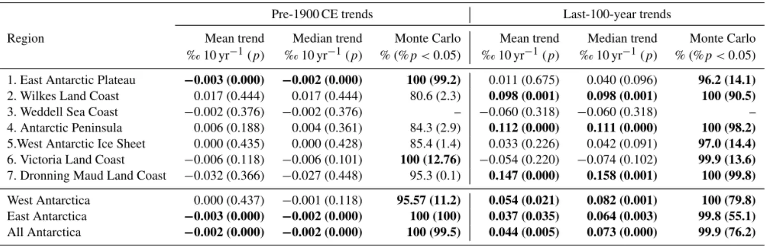
Table 2.Summary of trend statistics for isotopic anomalies using unweighted composites. Trends are expressed as isotopic anomalies, in per mille δ18O per decade units. Trends and their significance (p; based on the Student’s t statistic) are calculated using a linear additive model and reported for the mean and median composites. Monte Carlo testing is applied to 10 000 ensemble members based on the unweighted composite distributions, which are assessed to determine the percentage of trends with the same sign as the mean trend and the percentage with the same sign and a significance of p < 0.05. Bold values indicate mean and median trends with a significance of p < 0.05 and Monte Carlo simulations where significant; same-signed trends exceed 5 % of the ensemble.
Pre-1900 CE trends Last-100-year trends
Region Mean trend Median trend Monte Carlo Mean trend Median trend Monte Carlo
‰ 10 yr−1(p) ‰ 10 yr−1(p) % (%p < 0.05) ‰ 10 yr−1(p) ‰ 10 yr−1(p) % (%p < 0.05) 1. East Antarctic Plateau −0.003 (0.000) −0.002 (0.000) 100 (99.2) 0.011 (0.675) 0.040 (0.096) 96.2 (14.1) 2. Wilkes Land Coast 0.017 (0.444) 0.017 (0.444) 80.6 (2.3) 0.098 (0.001) 0.098 (0.001) 100 (90.5) 3. Weddell Sea Coast −0.002 (0.376) −0.002 (0.376) – −0.060 (0.318) −0.060 (0.318) – 4. Antarctic Peninsula 0.006 (0.188) 0.004 (0.361) 84.3 (2.9) 0.112 (0.000) 0.111 (0.000) 100 (98.2) 5.West Antarctic Ice Sheet 0.000 (0.435) 0.000 (0.428) 85.4 (1.4) 0.033 (0.226) 0.042 (0.091) 97.0 (14.4) 6. Victoria Land Coast −0.006 (0.118) −0.006 (0.101) 100 (12.76) −0.054 (0.220) −0.074 (0.102) 99.9 (13.6) 7. Dronning Maud Land Coast −0.032 (0.366) −0.027 (0.448) 95.3 (0.1) 0.147 (0.000) 0.158 (0.001) 100 (99.8) West Antarctica 0.000 (0.437) −0.001 (0.118) 95.57 (11.2) 0.054 (0.021) 0.082 (0.001) 100 (79.8) East Antarctica −0.003 (0.000) −0.002 (0.000) 100 (100) 0.037 (0.035) 0.064 (0.003) 99.8 (55.1) All Antarctica −0.002 (0.000) −0.002 (0.000) 100 (99.5) 0.044 (0.005) 0.073 (0.000) 99.9 (76.2)
trends that have been identified in other continental recon-structions (PAGES 2k Consortium, 2013) and in the global oceans (McGregor et al., 2015).
Isotopic trends in the last 100 years of the unweighted composites show significant positive trends across a number of regions. In particular, significant isotopic trends, indica-tive of climate warming, are evident in the unweighted com-posites for the Antarctic Peninsula and the Wilkes Land and Dronning Maud Land coasts. The West Antarctic Ice Sheet region does not display a significant (p < 0.05) positive trend in the mean or median of the unweighted composites, but the Monte Carlo analysis across the distribution of isotopic data within each 10-year bin suggests that positive trends are produced in 99.5 % of the 10 000 simulations and are significant (p < 0.05) more often than can be explained by chance alone (20.5 % of simulations). Similarly, the Victo-ria Land–Ross Sea region shows a negative but insignificant trend in the mean and median composites, but in the Monte Carlo simulations this negative (cooling) trend is produced in 99.9 % of ensemble members and is significant in 13.6 % of ensemble members. The apparent inverse isotopic trends during the last century between the Victoria Land–Ross Sea region and the West Antarctic Ice Sheet and Antarctic Penin-sula regions may be indicative of dynamical processes in the Amundsen Sea sector, which on interannual timescales are known to cause opposing climate anomalies between these regions.
The PAGES 2k Consortium (2013) study concluded that Antarctica was the only continent-scale region to not see the long-term cooling trend of the past 2000 years reverse to re-cent significant warming. However, on the regional scale ex-amined in this study recent significant warming is suggested by many of the unweighted isotopic composites, particularly
for coastal regions of Antarctica and the West Antarctic Ice Sheet. It should be stressed that these results are based only upon the simple unweighted compositing of the regional iso-topic data, and the significance of trends is further assessed in the following section after weighting of the individual ice core records based on how representative they are of isotopic and temperature variability within each climatic region.
4.1.2 Long-term trends in weighted reconstructions
To extend this trend analysis further, we next assess the pre-1900 CE (Fig. 5) trends in the temperature reconstructions produced by scaling the ice core data based on our differ-ent approaches (see Sect. 3.3.3). We estimate the uncertainty of the slope based on the ±2σ uncertainty in the regression parameters. The robustness of the slope estimation to indi-vidual data points was further checked by taking out 10 % of data points randomly and calculating the slope again, but the uncertainty estimate this yields is much smaller than the uncertainty based on regression parameters. The slopes ob-tained by each of the temperature scaling methods are pre-sented in Table 3. The uncertainty in the amplitude of the 0–1900 CE trend is dominated by the uncertainty in the tem-perature scaling of the composite. To make the discussion clear, we first focus on the trend in terms of normalized δ18O anomalies, with respect to the 1900–1990 CE periods, which circumvent the temperature scaling issues.
The period 0–1900 CE exhibits significant negative trends in most regions, from −0.4 to −1.3σ 1000 yr−1. The trend is largest in the West Antarctic Ice Sheet (−1.3 ± 0.2σ 1000 yr−1), Victoria Land (−0.9±0.4σ 1000 yr−1) and the Antarctic Plateau (−0.8 ± 0.3σ 1000 yr−1) regions. It is smaller but still significant for the Wilkes Land Coast
Figure 6.Histograms showing the distributions of all 100-year trends on normalized, weighted composites over the last 2000 years. Distribu-tions are shown for each climatic region, as well as for East, West and whole of Antarctica composites, and are calculated on 10-year-binned composites. The solid vertical lines represent the most recent 100-year trend in each reconstruction, and grey shading corresponds to the 5–95 % uncertainty range of the last 100-year trends. Only for the Antarctic Peninsula does the most recent 100-year trend stand out as unusual compared to the natural range of century-scale trends over the last 2000 years.
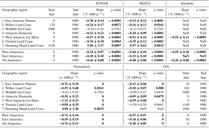
Table 3.Trend analysis of the period 0–1900 CE (or shorter depending on maximum record length) for the various temperature scaling approaches detailed in Sect. 3.4.
ECHAM NB2014 Borehole
Geographic region Start End Slope pvalue Slope pvalue Slope pvalue date date (◦C 1000 yr−1) (◦C 1000 yr−1) (◦C 1000 yr−1)
1. East Antarctic Plateau 0 1900 −0.38 ± 0.14 < 0.0001 −0.32 ± 0.12 < 0.0001 NaN NaN 2. Wilkes Land Coast 170 1900 −0.24 ± 0.17 0.0072 −0.16 ± 0.13 0.0161 NaN NaN 3. Weddell Sea Coast 1000 1900 −0.24 ± 0.54 0.3763 −0.12 ± 0.27 0.3763 NaN NaN 4. Antarctic Peninsula 0 1900 −0.52 ± 0.23 < 0.0001 −0.20 ± 0.09 < 0.0001 NaN NaN 5. West Antarctic Ice Sheet 0 1900 −0.47 ± 0.10 < 0.0001 −0.92 ± 0.16 < 0.0001 −0.55 ± 0.11 < 0.0001 6. Victoria Land Coast 0 1900 −0.34 ± 0.18 0.0003 −0.29 ± 0.12 < 0.0001 NaN NaN 7. Dronning Maud Land Coast 1530 1900 5.96 ± 3.27 0.0007 0.97 ± 0.62 0.0032 NaN NaN West Antarctica 0 1900 −0.24 ± 0.07 < 0.0001 −0.44 ± 0.10 < 0.0001 −0.55 ± 0.10 < 0.0001 East Antarctica 0 1900 −0.30 ± 0.10 < 0.0001 −0.32 ± 0.10 < 0.0001 NaN NaN All Antarctica 0 1900 −0.36 ± 0.08 < 0.0001 −0.40 ± 0.08 < 0.0001 −0.26 ± 0.06 < 0.0001
Normalized CPS
Geographic region Slope pvalue Slope pvalue Start End
(σ 1000 yr−1) (◦C 1000 yr−1) date date 1. East Antarctic Plateau −0.76 ± 0.28 0 −0.15 ± 0.06 0 10 1900 2. Wilkes Land Coast −0.59 ± 0.48 0.0161 −0.10 ± 0.07 0.008 180 1900 3. Weddell Sea Coast −0.41 ± 0.92 0.3763 −0.09 ± 0.27 0.4935 1000 1900 4. Antarctic Peninsula −0.50 ± 0.23 0 −0.09 ± 0.09 0.0479 0 1900 5. West Antarctic Ice Sheet −1.32 ± 0.23 0 −0.59 ± 0.08 0 0 1900 6. Victoria Land Coast −0.89 ± 0.39 0 −0.54 ± 0.58 0.0661 1140 1900 7. Dronning Maud Land Coast 4.98 ± 3.20 0.0032 NaN NaN 1890 1900
West Antarctica −0.76 ± 0.16 0 −0.55 ± 0.07 0 0 1900
East Antarctica −0.59 ± 0.19 0 −0.18 ± 0.06 0 10 1900
All Antarctica −0.76 ± 0.15 0 −0.38 ± 0.05 0 0 1900
(−0.6±0.5σ 1000 yr−1, p = 0.007) and Antarctic Peninsula (−0.5 ± 0.2σ 1000 yr−1). It is insignificant on the Weddell Sea Coast (p = 0.4), and the data set is not long enough to estimate millennial-scale trends on the Dronning Maud Land Coast. These observations indicate a broad-scale
cool-ing trend over the continent, which is comparable in ampli-tude to the variance over the past 100 years. As previously mentioned, the 0–1900 CE negative trend is largest in the normalized data sets for the West Antarctic Ice Sheet region, but this feature masks subregional-scale differences, with


![[PDF] Apprendre à travailler avec Microsoft Virtual PC en Pdf | Formation informatique](data:image/gif;base64,R0lGODlhAQABAIAAAP///wAAACH5BAEAAAAALAAAAAABAAEAAAICRAEAOw==)