HAL Id: hal-01583951
https://hal.archives-ouvertes.fr/hal-01583951
Submitted on 27 Oct 2020
HAL is a multi-disciplinary open access
archive for the deposit and dissemination of
sci-entific research documents, whether they are
pub-lished or not. The documents may come from
teaching and research institutions in France or
abroad, or from public or private research centers.
L’archive ouverte pluridisciplinaire HAL, est
destinée au dépôt et à la diffusion de documents
scientifiques de niveau recherche, publiés ou non,
émanant des établissements d’enseignement et de
recherche français ou étrangers, des laboratoires
publics ou privés.
of δ13CH4 and C2H6 when using a cavity ring-down
spectrometer at industrial sites
Sabina Assan, Alexia Baudic, Ali Guemri, Philippe Ciais, Valerie Gros, Felix
R. Vogel
To cite this version:
Sabina Assan, Alexia Baudic, Ali Guemri, Philippe Ciais, Valerie Gros, et al.. Characterization of
interferences to in situ observations of δ13CH4 and C2H6 when using a cavity ring-down spectrometer
at industrial sites. Atmospheric Measurement Techniques, European Geosciences Union, 2017, 10 (6),
pp.2077 - 2091. �10.5194/amt-10-2077-2017�. �hal-01583951�
https://doi.org/10.5194/amt-10-2077-2017 © Author(s) 2017. This work is distributed under the Creative Commons Attribution 3.0 License.
Characterization of interferences to in situ observations of
δ
13
CH
4
and C
2
H
6
when using a cavity ring-down
spectrometer at industrial sites
Sabina Assan, Alexia Baudic, Ali Guemri, Philippe Ciais, Valerie Gros, and Felix R. Vogel
Laboratoire des Sciences du Climat et de l’Environnement, Chaire BridGES, UMR CNRS-CEA-UVSQ, Gif-sur-Yvette, Ile-de-France, 91191, France
Correspondence to:Sabina Assan (sabina.assan@lsce.ipsl.fr) Received: 2 August 2016 – Discussion started: 19 December 2016
Revised: 8 March 2017 – Accepted: 15 March 2017 – Published: 7 June 2017
Abstract. Due to increased demand for an understanding of CH4emissions from industrial sites, the subject of cross
sensitivities caused by absorption from multiple gases on δ13CH4and C2H6measured in the near-infrared spectral
do-main using CRDS has become increasingly important. Ex-tensive laboratory tests are presented here, which charac-terize these cross sensitivities and propose corrections for the biases they induce. We found methane isotopic mea-surements to be subject to interference from elevated C2H6
concentrations resulting in heavier δ13CH4 by +23.5 ‰
per ppm C2H6/ppm CH4. Measured C2H6is subject to
ab-sorption interference from a number of other trace gases, predominantly H2O (with an average linear sensitivity of
0.9 ppm C2H6per % H2O in ambient conditions). Yet, this
sensitivity was found to be discontinuous with a strong hys-teresis effect and we suggest removing H2O from gas
sam-ples prior to analysis. The C2H6calibration factor was
cal-culated using a GC and measured as 0.5 (confirmed up to 5 ppm C2H6). Field tests at a natural gas compressor station
demonstrated that the presence of C2H6in gas emissions at
an average level of 0.3 ppm shifted the isotopic signature by 2.5 ‰, whilst after calibration we find that the average C2H6: CH4ratio shifts by +0.06. These results indicate that,
when using such a CRDS instrument in conditions of ele-vated C2H6for CH4source determination, it is imperative to
account for the biases discussed within this study.
1 Introduction
With increasing efforts to mitigate anthropogenic greenhouse gas emissions, opportunities to reduce leaks from fossil fuel derived methane (ffCH4) are of particular importance as
they currently account for approximately 30 % of all an-thropogenic methane emissions (Kirschke et al., 2013). At present, technically feasible mitigation methods hold the po-tential to half future global anthropogenic CH4emissions by
2030. Of this mitigation potential more than 60 % can be re-alized in the fossil fuel industry (Hoglund-Isaksson, 2012). However, for effective implementation, sources, locations and magnitudes of emissions must be well known.
The global increase in the production and utilization of natural gas, of which methane is the primary component, has brought to light questions in regards to its associated fugitive emissions, i.e. leaks. Recent estimates of CH4leaks
vary widely (1–10 % of global production; Allen, 2014) and US inventories of natural gas CH4emissions have
uncertain-ties of up to 30 % (US EPA, 2016). In addressing this is-sue, the ability to distinguish between biogenic and different anthropogenic sources is of vital importance. For this rea-son methane isotopes (δ13CH4)are commonly used to better
understand global and local emissions, as demonstrated in a number of studies (Lamb et al., 1995; Lowry et al., 2001; Hiller et al., 2014). The discrimination of sources with rel-atively close isotopic composition such as oil-associated gas and natural gas, which can have isotopic signatures separated by only ∼ 4 ‰ (Stevens and Engelkemeir, 1988), requires precise and reliable δ13CH4measurements.
Figure 1. Flow chart illustrating the steps involved to calibrate C2H6and δ13CH4. The number in the top right-hand corner cor-responds to the subsection in which the methods of each step are explained in detail.
Ethane (C2H6)is a secondary component in natural gas
and can be used as a marker to distinguish between differ-ent CH4sources. Use of the C2H6: CH4ratio provides a
ro-bust identifier for the gas of interest. Recent findings in the US found coal bed C2H6: CH4ratios ranging between 0 and
0.045, while dry and wet gas sources displayed differing ra-tios of < 0.06 and > 0.06 respectively (Yacovitch et al., 2014; Roscioli et al., 2015).
Laser spectrometers, especially those based on cavity ring-down spectroscopy (CRDS), are now a common deployment for site-scale CH4measurement campaigns (Yvon-Lewis et
al., 2011; Phillips et al., 2013; Subramanian et al., 2015). However, with the advent of such novel technologies, there is a risk of unknown interference from laser absorption which can create biases in measurements. Some examples of this are discussed in Rella et al. (2015) and many others (e.g. Malowany et al., 2015; Vogel et al., 2013; Nara et al., 2012). Using a CRDS instrument we show that the presence of C2H6
causes significant interference to the measured13CH4
spec-tral lines, thus resulting in shifted reported δ13CH4values.
We propose a method to correct these interferences and test it on measurements of natural gas samples performed at an industrial natural gas site.
The CRDS instruments used throughout this study are Pi-carro G2201-i analysers (PiPi-carro INC, Santa Clara, USA) which measure gases including CH4, CO2, H2O, and,
al-though not intended for use by standard users, C2H6. This
model measures in three spectral ranges: lasers measuring spectral lines at roughly 6057, 6251 and 6029 cm−1are used to quantify mole fractions of12CH4,12CO2and13CO2, and 13CH
4, H2O and C2H6 respectively. The spectrograms are
fit with two non-linear models in order to determine con-centrations; the primary fit excludes the model function of C2H6while the second includes this function, thus adding the
ability to measure C2H6(Rella et al., 2015). Such a method
for measuring C2H6concentrations is crude, thus the
uncali-brated C2H6concentration data are stored in private archived
files which until now have been used primarily for the detec-tion of sample contaminadetec-tion. The measurements of δ13CH4
and δ13CO2are calculated using the ratios of the
concentra-tions of12CH4,13CH4,12CO2and13CO2respectively.
An experimental procedure is presented here which cor-rects the interference caused by C2H6 on the retrieval of
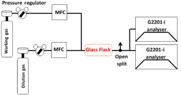
Figure 2. General set-up. The dilution and working gas are con-nected via two MFCs to two CRDS instruments in parallel. In red is the placement of an optional glass flask used for the C2H6 cali-bration only. The flow is greater than that of the instruments’ inlets. Therefore an open split is included to vent additional gas and retain ambient pressure at the inlets.
δ13CH4 using such a CRDS instrument for application to
in situ or continuous measurements of δ13CH4strongly
con-taminated by C2H6, i.e. in the vicinity of ffCH4sources. The
step-by-step procedure of the experimental methods devel-oped to quantify the cross sensitivities and the proposed cal-ibration for δ13CH4and C2H6are depicted in Fig. 1 and
pre-sented in detail in Sect. 2. Section 3 encompasses a discus-sion of the results, including an analysis of the instrumental responses for two spectrometers with an evaluation of the sta-bility and repeatasta-bility of the suggested corrections. Finally, field measurements were performed at a natural gas compres-sor station where the aim was to identify emissions between two natural gas pipelines. In Sect. 5 the importance of the corrections for field measurements is demonstrated by ap-plying our methods to data retrieved during this period while also revealing the instruments’ potential to measure C2H6.
2 Methods
The purpose of laboratory tests was to characterize the in-struments’ response to concentration changes in gases found at fossil fuel sites (e.g. gas extraction or compressor stations), specifically, the cross sensitivities of CO2, CH4and H2O on
C2H6and of C2H6on δ13CH4. Presumably there are
addi-tional gases with the potential for interference; this study fo-cuses on those reported to have a significant effect on C2H6
and δ13CH4measurements by Rella et al. (2015). We also
define and describe a new procedure to calibrate both C2H6
and δ13CH4.
In the following chapter the general set-up used for the majority of experiments is described, after which we enter a more detailed description of the processes involved in each step.
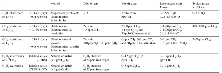
Table 1. Description of the gas mixtures used to determine the cross-sensitivities of the interference of CH4, H2O and CO2on C2H6and the interference of C2H6on δ13CH4. The respective ranges spanned during laboratory tests, and the typical range at a natural gas site are noted on the right-hand side.
Method Dilution gas Working gas Lab concentration Typical range
Range at NG site
H2O interference < 0.16 % (dry) Magnesium perchlorate N/A Ambient air 0–0.5 % H2O 0–2 % H2O
on C2H6 ≥0.16 % (wet) Dilution series Zero air 0.25–2.5 % H2O
& humidifier
CO2interference < 0.16 % (dry) Dilution series Zero air 2000 ppm CO2, 0–1500 ppm CO2 400–1000 ppm CO2
on C2H6 ≥0.16% (wet) Dilution series & 1.7 ppm CH4, < 1 ppb C2H6and 0–1500 ppm CO2,
humidifier 50 ppb CO in natural air 0.5–1.5 % H2O
CH4interference < 0.16 % (dry) Dilution series & Zero air 6 ppm CH4, 360 ppm CO2, 0–6 ppm CH4 2–20 ppm CH4
on C2H6 ascarite 310 ppb N2O, < 1 ppb C2H6 and 50 ppb CO in natural air 0–6 ppm CH4, 1 %H2O ≥0.16 % (wet) Dilution series, ascarite
& humidifier
C2H6interference Dilution series Natural air matrix C2H6standard 0–1.5 ppm C2H6/ 0–0.3 ppm C2H6/
on δ13CH
4 (CRDS) (< 1 ppb C2H6) of 52 ppm in nitrogen ppm CH4 ppm CH4
C2H6calibration Dilution series Natural air matrix C2H6standard 0–5 ppm C2H6 0.3–3 ppm C2H6
(CRDS & GC) (< 1 ppb C2H6) of 52 ppm in nitrogen
2.1 Experimental set-up 2.1.1 Method
Each cross sensitivity is measured by creating a gas dilution series designed to control the concentrations of the gas re-sponsible for the interference in steps while keeping concen-trations of the other gas components constant (in particular the component subject to interference). The instrument re-sponse was evaluated for a large range of concentrations and different combinations of gas components. An example of such a measurement time series can be seen in Fig. S1 in the Supplement. The experimental set-up used includes two CRDS instruments (Picarro G2201-i) running in parallel in a laboratory at ambient conditions (25◦C, 100 m above sea level; a.s.l). The instruments were used in iCO2-iCH4auto
switching mode, of which we consider only the “high pre-cision” mode of δ13CH4 throughout the study. For the
di-lution series, a working gas is diluted in steps using a set-up of two mass flow controllers (MFC; El-flow, Bronkhorst, Ru-urlu, the Netherlands), as shown in Fig. 2. A T-junction splits the gas flow to both instruments; the total flow is greater than the flow drawn into the instruments. Hence to maintain an in-let pressure close to ambient, the set-up includes an open split to vent additional gas. In order to assess variability and error, each experiment is repeated a minimum of three times con-secutively. To detect instrumental drift between experiments, a target gas is measured before commencing each dilution sequence. An overview of each targeted cross interference, with information on the gases used and ranges spanned in laboratory tests, can be found in Table 1.
2.1.2 Gases
Throughout the experiments, four categories of gas were used: a zero air gas with measured residual concentrations of
< 1 ppm CO2, < 30 ppb CH4 , ≈ 170 ppb CO, < 1 ppb C2H6
(Deuste-Steininger,Walldorf, Germany), working gases with variable concentrations of CO2and CH4in a natural air
ma-trix (Deuste-Steininger,Walldorf, Germany), a C2H6
stan-dard of 52 ppm in nitrogen (National Physics Laboratory (NPL), Teddington, United Kingdom), and dried ambient air in 40L aluminium cylinders filled using an oil-free RIX compressor (RIX industries, Benicia, USA). Details of the gas mixture used in each dilution series depends on the re-sponse targeted within the experiment. This information can be found in Table 1 and is also discussed in further detail throughout this chapter.
2.2 Determination of C2H6corrections from H2O, CH4
and CO2interference
The value of C2H6based on the standard CRDS data
pro-cessing package (hereafter, the raw value) is biased by cross-sensitivities with H2O, CO2 and CH4. Experiments were
conducted at different constant C2H6concentrations so that
any shifts in the raw C2H6are due to the cross sensitivity to
other components in the measured samples. To alter the wa-ter vapour content of a sample, the experimental set-up de-scribed in Fig. 2 was modified by incorporating a humidifier. The humidifier consists of a liquid flow controller (Liqui-flow, Bronkhorst, Ruurlu, the Netherlands) and a mass flow controller (El-flow, Bronkhorst, Ruurlu, the Netherlands) fed into a controlled evaporator mixer (CME) (Bronkhorst, Ru-urlu, the Netherlands). The tube departing the CME contains a gas flow of 2 L min−1and is heated to 40◦C to prevent any condensation. A short description and diagram of the humid-ifying bench can found in Laurent et al. (2015).
The H2O interference on C2H6 was measured by using
the humidifier to vary the H2O content of zero air gas in
the range of 0.25–2.5 % H2O, representing the range of real
humidity below 0.2 % H2O, a range frequently reached when
measuring gas cylinders or dried air. This low range was at-tained using a H2O scrubber (Magnesium Perchlorate, Fisher
Scientific, Loughborough, UK) connected to the CRDS in-strument inlet while measuring ambient air. As the efficiency of the scrubber decreases over time, a slow increase of H2O
spanning low concentrations in the range of 0–0.5 % can be observed.
The CH4 interference on C2H6 was measured by
creat-ing a dilution series of variable CH4content using zero air
and a working gas of 6 ppm CH4, 360 ppm CO2, 310 ppb
N2O and 50 ppb CO in natural air. Methane concentrations
ranged from 0 to 6 ppm. To keep other causes of interference at a minimum, the gas mixture passed through two scrub-bers: the first a CO2scrubber (Ascarite(ii), Acros Organics,
USA) and the second a H2O scrubber (Magnesium
Perchlo-rate, Fisher Scientific, Loughborough, UK). As an indepen-dent check on the linearity of the response functions, each dilution sequence was repeated at two humidities (0 % H2O
and 1 % H2O) and four C2H6concentrations (between 0 and
1.5 ppm).
The CO2interference on C2H6was measured with a
dilu-tion series ranging 0–1500 ppm CO2created by mixing zero
air and a working gas of 2000 ppm CO2, 1.7 ppm CH4and
50 ppb CO in natural air. Any interference due to CH4was
accounted for during data processing. This test was repeated at four water vapour levels (0, 0.5, 1 and 1.5 %) and five C2H6concentrations (between 0 and 2.5 ppm).
2.3 C2H6calibration set-up
In order to correctly use the C2H6data from CRDS
instru-ments, the data must be calibrated to an internationally recog-nized scale. To achieve this, the set-up described in Sect. 2.1 was modified to include the filling of removable samples (1 L glass flasks), the concentrations of which could be indepen-dently verified, as shown in Fig. 2. A gas mixture using the C2H6standard and an ambient air cylinder was created via
two MFCs before passing through the flask on its way to the instruments’ inlets. Each step in the dilution series requires an individual flask, which was flushed for 20 min and then analysed for 10 min with an average precision of 0.02 ppm C2H6 on the CRDS instrument. The flask is subsequently
sealed and removed for analysis on a gas chromatograph (GC) (Chrompack Varian 3400, Varian Inc, USA) which uses National Physics Laboratory (NPL) standards and has an un-certainty better than 5 %. The system is described in more detail in Bonsang and Kanakidou (2001).
In total 17 flasks were filled with gas mixtures spanning from 0 to 5 ppm C2H6, covering the range expected near a
leak of ffCH4(Gilman et al., 2013; Jackson et al., 2014). In
order to calibrate the linearity of the response at very high concentrations which may be expected from pure natural gas samples, we conducted a measurement at 100 % of the C2H6
standard (52 ppm ± 1 ppm).
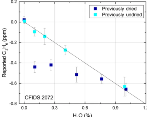
Figure 3. An example of the results from a H2O interference ex-periment spanning the range 0–1 % H2O. The reported C2H6is al-tered due to the addition of water vapour when measuring zero air (< 1 ppb C2H6). Dark and light blue markers signify the response when dried and undried ambient air have been measured overnight by the instrument prior to the experiment respectively. Error bars signify the standard deviation of each measurement.
2.4 Determining the correction for δ13CH4
Measured δ13CH4is altered in the presence of C2H6. To
un-derstand the magnitude of this effect, experiments were con-ducted using the method described in Sect. 2.1. The dilution series uses the C2H6standard and a cylinder filled with
ambi-ent air, i.e. with a negligible C2H6mixing ratio (< 1 ppb), to
create concentration values spanning from 0 to 4 ppm C2H6.
As there is only one source of CH4in the experiment, the
ad-dition of C2H6should not affect the value of δ13CH4; hence
any change seen is an apparent shift of δ13CH4due to C2H6
interference. This concentration range was chosen as it en-compasses a C2H6: CH4ratio of 0 to 1, well within the likely
range to be measured from fossil fuel sources (Yacovitch et al., 2014).
2.5 Calibration of δ13CH4
The reported δ13CH4was calibrated to Royal Holloway
Uni-versity of London (RHUL) scale using four calibration gases spanning −25 to −65 ‰ that were created by different di-lutions of pure CH4and CO2with ambient air. The aliquots
were measured multiple times by isotope ratio mass spec-trometry (IRMS) at RHUL. The precision for δ13CH4,
ob-tainable with this IRMS, is reported as 0.05 ‰ – detailed in-formation on the measurement system can be found in Fisher et al. (2006). The calibration factor is determined from a lin-ear regression and calibrations were performed once a day for 3 consecutive days before and after the laboratory experi-ments. A target gas was measured regularly to track any drift in δ13CH4as an independent check on the calibration quality.
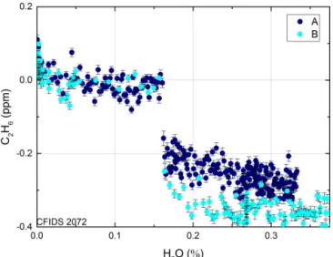
Figure 4. The discontinuity seen for instrument CFIDS 2072 for two repetitions denoted by different colours. After the discontinuity at 0.16 % the subsequent slope clearly differs between the two rep-etitions. Both instruments display a discontinuity at 0.16 % H2O. Each point represents a 1 min average, the error bars represent the standard deviation of the raw data.
3 Results and discussion
This study focuses on determining a reliable correction and calibration scheme for a Picarro G2201-i when measuring methane sources with C2H6interference. Findings from the
experiments described in Sect. 2 are discussed in detail here. In order to calibrate δ13CH4 and C2H6 values, there are
a series of corrections that must take place beforehand (see Fig. 1). The initial correction to be applied is on C2H6due to
interference from CH4, CO2and H2O. Particular emphasis is
placed on this correction due to the discovery of significant non-linear behaviour in the presence of H2O, CH4and CO2
in the sample gas. Once the C2H6has been corrected, the
cal-ibration of C2H6using independent GC measurements, the
C2H6interference correction on δ13CH4and finally the
cali-bration of δ13CH4can be effected.
For our results to be applicable to future studies we ex-amine the inter-instrument variability and stability over time, compare our results to current literature and discuss the un-certainties attributed to our results. Throughout this study we refer to raw, uncorrected C2H6 and δ13CH4 concentrations
as “reported” to highlight that they may be influenced by in-terferences and are uncorrected. Within this section negative C2H6concentrations are often mentioned. We note that this
is the “reported” C2H6concentration by the instrument.
Un-less otherwise stated, the standard deviation reported is cal-culated from 1 min averages and depicted as error bars within figures.
3.1 Correcting reported C2H6
3.1.1 H2O interference on C2H6
H2O content was found to be the dominating source of
in-terference to reported C2H6; its presence decreases the
re-ported concentration of C2H6with increasing H2O
concen-tration. Furthermore, the response function exhibits a hys-teresis effect, which, although small, can be considerable when changing from dry to undried air samples (e.g. be-tween dry calibration gas and undried ambient air). There are two distinct instrumental responses, depending on whether dried or undried ambient air are being measured during the night preceding the experiment, which are depicted in Fig-ure 3 by dark and light blue markers respectively. When the CRDS instrument measures dry air prior to the experi-ment, a discontinuity is observed at 0.16 % H2O. Figure 4
shows this effect in more detail; prior to 0.16 % H2O the
re-sponse function exhibits a stable linear rere-sponse. The correc-tion within this low range was found to be the same for both instruments, 0.44 ± 0.03 ppm C2H6/% H2O. After passing
the 0.16 % H2O threshold, the response exhibits a
discon-tinuity with a magnitude and subsequent slope that are also dependent on the air moisture beforehand. This is seen in Fig. 4 whereby the discontinuity of two repetitions (A and B depicted by dark and light blue markers respectively) dif-fers in magnitude by 0.1 ppm reported C2H6. The
discon-tinuity occurs when the instrument passes the 0.16 % H2O
threshold, both when moving from dry to wet air and vice versa (see Fig. S2). If measuring undried air before the ex-periment, the interference due to H2O can be described well
by a linear response (light blue markers in Fig. 3) and poten-tially causes large biases from the true C2H6. For example, if
measuring at 1 % H2O, both instruments display a change
in reported C2H6 of approximately −0.9 ppm. The
re-sponse function calculated for instruments CFIDS 2072 and 2067 differed, showing −0.72 ± 0.03 ppm C2H6/% H2O
and −1.00 ± 0.01 ppm C2H6/% H2O with R2values of 0.98
and 0.99 respectively. The hysteresis effect is evident when measuring with undried air; the slope was seen to shift after each repetition, in total by 0.1 ppm C2H6/% H2O.
3.1.2 CO2interference on C2H6
For both instruments an increase in the CO2
concentra-tion results in lower reported values of C2H6, and it is
furthermore apparent that the magnitude of this interfer-ence is dependent on air humidity. For a dry sample gas (H2O < 0.16 % – demonstrated in the left-hand column of
Fig. 5), the interference for both instruments is found to be highly stable and well characterized by a linear slope of 1 × 10⁻⁴±1 × 10⁻⁵ppm C2H6/ppmCO2 with a R2 value
of 0.9. There was no measurable difference in slope at any of the C2H6 concentrations tested (see Fig. S3). In
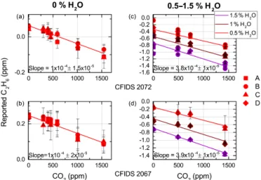
right-Figure 5. Relationship between reported C2H6and concentration changes of CO2for instruments CFIDS 2072 and 2067 at vary-ing values of H2O, at 0 ppm C2H6(within our instrumental pre-cision). For each plot the bottom axis indicates the concentration of the targeted gas (CO2). Plots (a) and (b) are at 0 % H2O, (c) and (d) are experiments at varying humidities, distinguishable by colour. The legend denotes repetitions of the experiment. The error bars in each plot denote the standard deviation of each measurement. The R2values for the experiments at 0 % H2O are 0.9 and 0.8 for all other H2O experiments for both instruments.
hand column of Fig. 5), measurements exhibit a higher scatter between repetitions. This is mainly attributed to a drifting intercept; however the experiments also show a smaller R2 of 0.8. We calculate a characteristic linear slope of 3.8 × 10⁻⁴±1 × 10⁻⁵ppm C2H6/ppm CO2 and
3.9 × 10⁻⁴±1 × 10⁻⁵for ≥ 0.5 % water vapour for instru-ments CFIDS 2072 and 2069 respectively. Therefore, when measuring undried ambient air, the presence of CO2 at a
level near 400 ppm will induce a shift in the reported C2H6
of approximately −0.15 ppm C2H6, whereas if the air is
dried the reported shift is much smaller, at approximately −0.04 ppm C2H6.
3.1.3 CH4interference on C2H6
The CH4effect on C2H6, as shown in Fig. 6, is less
promi-nent by at least an order of magnitude than both the H2O
and CO2 interferences. At dried ambient CH4
concentra-tions a typical change in reported C2H6 of approximately
−0.008 ppm is observed within both instruments. Dried air experiments show a high scatter of points between repeti-tions, and R2 values of 0.4 and 0.6 for instruments CFIDS 2072 and 2067 respectively are calculated. Despite its large uncertainty, the data suggest that both instruments display a similar response with a statistically significant slope within the range of C2H6 concentrations tested (see Fig. S3). In
light of this we use a weighted mean to calculate a linear response of 9 × 10⁻³±2 × 10⁻³ppm C2H6/ppm CH4
for dry air measurements for CFIDS 2067, and
Figure 6. Relationship between reported C2H6and concentration changes of CH4 for both instruments at 0 ppm C2H6(within our instrumental precision). For each plot, the bottom axis indicates the increase in concentration of the targeted gas. The vertical bars in each plot denote the standard deviation of each point. The legend denotes repetitions of the experiment. Plots (a) and (b) are at 0 % H2O. The R2values are 0.4 and 0.6 for instruments CFIDS 2072 and 2067. Plots (c) and (d) show the response at 1 % H2O. These two plots have a R2value of 0.2.
7 × 10⁻³±5 × 10⁻³ppm C2H6/ppm CH4 for CFIDS
2072. The results obtained at 1 % H2O show little
correla-tion (as shown in the right-hand column of Fig. 6), with both instruments displaying a R2 value of 0.2. An ANOVA test suggests the slopes are not significantly different from zero; thus we omit a CH4correction for this case.
3.1.4 Combining the CO2, CH4and H2O correction on
C2H6
To fully take into account all (known) C2H6
cross-sensitivities, the corrections to reported C2H6 need to be
combined. Due to the non-linearity of the discontinuity in reported C2H6 at 0.16 % H2O and its subsequent slope we
choose to report correction coefficients for the two found linear regimes, i.e. for continuous measurements with sam-ple humidities below 0.16 % and samsam-ple humidities above 0.16 %. Within each range the proposed correction formula is given as follows:
(C2H6)CORRECTED=(C2H6)RAW+A∗(H2O) + B∗(CH4)
+C∗(CO2). (1)
If the humidity is limited to less than 0.16 % before and during measurements, A = 0.44 ± 0.03 ppm C2H6/% H2O,
B = 8 × 10⁻³±2 × 10⁻³ppm C2H6/ppm CH4, C =
1 × 10⁻⁴±1 × 10⁻⁵ppm C2H6/ppm CO2. Both
instru-ments demonstrated good agreement for all the correction factors calculated at < 0.16 % H2O.
Corrections for measurements undertaken at concen-trations higher than or equal to 0.16 % H2O are A =
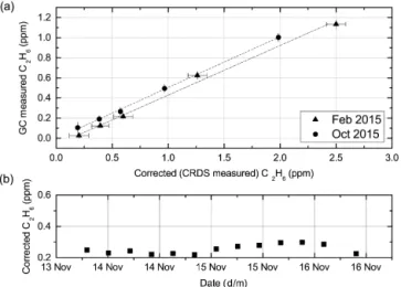
Figure 7. (a) Ethane calibration calculated from measurements of flask samples by both the GC and CRDS. The x-axis is the cor-rected C2H6 (C2H6 COR) using the corrections described previ-ously. The y-axis is the C2H6as measured by a manual GC. The error bars indicate the standard deviation of each flask measure-ment, for certain flasks error bars are smaller than their respective markers. (b) 30 min target measurements over a period of 4 days, from 13 to 16 November 2015. The standard error of each target is smaller than the plotted marker. The baseline C2H6is seen to drift with time.
0.7 ± 0.03 ppm C2H6/% H2O, B = 0 ppm C2H6/ppm
CH4, C = 3.8 × 10⁻⁴±2 × 10⁻⁵ ppm C2H6/ppm CO2
for CFIDS 2072 and A = 1 ± 0.01 ppm C2H6/% H2O,
B = 0 ppm C2H6/ppm CH4, C = 3.9 × 10⁻⁴±2 × 10⁻⁵
ppm C2H6/ppm CO2for CFIDS 2067.
3.2 C2H6calibration
To make use of the corrected C2H6 it should be
cali-brated to match an internationally recognized scale. This is achieved by measuring whole-air samples by CRDS and in-dependently on a calibrated gas chromatograph, as discussed within Sect. 2. The calibration factor is determined by com-paring the corrected C2H6resulting from CRDS and C2H6
as confirmed by the GC and plotted in Fig. 7a. The relation-ship was found to be linear throughout the range of 0–5 ppm C2H6with a slope of 0.505 ± 0.007 and 0.52 ± 0.01 for
in-struments CFIDS 2072 and 2067 respectively. The results are reported in Table 2 from which we can see the intercept of the calibration for instrument CFIDS 2072 shifts between the experiment in February and that in October, while the slope remains constant throughout the measured time period. The change in the intercept is attributed to a C2H6baseline drift
which we have monitored over time using regular target gas measurements; an example is given in Fig. 7b. To account for this drift and any elevated baselines (such as that of CFIDS 2067 – see Table 2), a regular measurement of a working gas is necessary, from which the instrument offset can be calcu-lated. For the full calibration, we thus suggest using Eq. (2),
Figure 8. During a dilution sequence of ambient gas with C2H6, the CH4 concentration decreases from its nominal concentration 1948.7 ppb ± 0.32 ,ppb as the contribution from C2H6is increased. Thus both12CH4and13CH4undergo a similar decrease as the gas is diluted. However, what is observed is an increase in the reported value of13CH4, suggesting C2H6interference. The12CH4axis is plotted to the left in light green, whereas the13CH4axis is plotted to the right in dark green at a different scale. Error bars represent the standard deviation, the12CH4markers are larger than their as-sociated error bars.
where D is the calibration factor (slope) for the instrument, i.e. for CFIDS 2072 D = 0.505 ± 0.007 and 1 (WGS) the baseline drift determined using the working gas.
(C2H6)calibrated=D∗((C2H6)corrected−1(WGS)) (2)
3.3 δ13CH4correction
By measuring the shift of the reported δ13CH4 in C2H6
-contaminated samples, we have observed that the instrument reports heavier values of δ13CH4 in the presence of C2H6.
The shift is a result of increased reported13CH4 in
sam-ples containing C2H6(see Fig. 8). This is most likely caused
by the overlapping of spectral lines within the 6029 wave number region (Rella et al., 2015). We calculate the δ13CH4
correction by taking the slope of 1δ13CH4 (the difference
between the reported δ13CH4 and the initially reported one
of the C2H6-free gas) and the corrected C2H6to CH4ratio.
The ratio is used to permit the calculation of the δ13CH4
re-sponse function per ppm CH4 as the magnitude of
interfer-ence is dependent on CH4concentration (Rella et al., 2015).
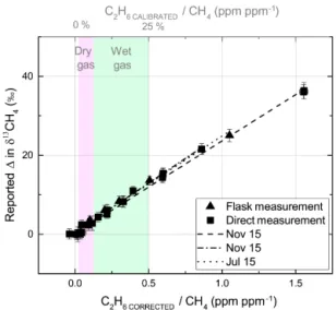
The significance of the interference on δ13CH4
concentra-tions is illustrated in Fig. 9; as the C2H6: CH4ratio increases,
the change in the reported δ13CH4increases linearly. Results
obtained from tests carried out throughout the year, for both instruments are noted in Table 3 and plotted in Fig. 9. The correction equation can be expressed as follows:
Table 2. Summary of C2H6calibration factors calculated for both instruments CFIDS 2072 and 2067. CFIDS 2072 CFIDS 2067 C2H6 Slope Intercept Slope Intercept
Calibration (ppm) (ppm)
Feb,15 0.49 ± 0.03 0.00 ± 0.01
Oct,15 0.51 ± 0.01 −0.06 ± 0.04 0.52 ± 0.01 −0.12 ± 0.01
Table 3. The various response functions calculated for the δ13CH4correction due to C2H6. CFIDS 2072 CFIDS 2067
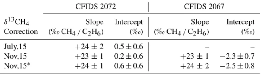
δ13CH4 Slope Intercept Slope Intercept Correction (‰ CH4/C2H6) (‰) (‰ CH4/C2H6) (‰) July,15 +24 ± 2 0.5 ± 0.6 – – Nov,15 +23 ± 1 0.2 ± 0.6 +23 ± 1 −2.3 ± 0.7 Nov,15∗ +24 ± 1 0.6 ± 0.6 +24 ± 2 −2.5 ± 0.8 ∗Flask measurement. (δ13CH4)CORRECTED=(δ13CH4)RAW −E∗C2H6 CORRECTED/CH4+F, (3)
where E is the slope of the response function and F is the in-tercept. E and F are +23.6 ± 0.4 ‰ ppm CH4/ppm C2H6
and approximately +0.4 ± 0.2 ‰ for instrument CFIDS 2072 and +23.3 ± 0.7 ‰ ppm CH4/ppm C2H6and
approx-imately −2.4 ± 0.4 ‰ for instrument CFIDS 2067 respec-tively. These corrections contain the inherent δ13CH4offset
of the instrument. When calibrating the δ13CH4to a known
scale (as described in Sect. 2.5) any instrumental offset will be incorporated within the calibration. Therefore, the correc-tion equacorrec-tions can be simplified to
(δ13CH4)CORRECTED=(δ13CH4)RAW
−E∗C2H6 CORRECTED/CH4. (4)
Also highlighted in Fig. 9 is the typical measurement range for the majority of ffCH4 sources related to dry and wet
natural gas relative to calibrated C2H6/CH4 ratios given
on the upper abscissa, whereby dry gas refers to natu-ral gas that occurs in the absence of condensate/liquid hy-drocarbons (C2H6: CH4=1–6 %) while wet gas typically
contains higher concentrations of complex hydrocarbons (C2H6: CH4> 6 %; Yacovitch et al., 2014). It is clear that
within this range the bias on methane isotopic signatures is significant; dry gas will alter the reported δ13CH4 by 0.8–
4 ‰, while wet gas can cause a shift of up to 13 ‰ depending on its C2H6: CH4ratio.
3.4 δ13CH4calibration
Full instrument calibrations as described in Sect. 2.4 were performed once in 2014 and once in 2015. The δ13CH4
val-ues obtained for the calibration gases by RHUL are measured
by IRMS and are therefore not subject to interferences. The calibration gas aliquots were measured with an average stan-dard deviation of 0.03 ‰. To calibrate δ13CH4 CORRECTED,
the δ13CH4 CORRECTED was calculated for each calibration
gas and used within the linear regression. The calibrations were linear with R2> 0.99 on both occasions and no change (within our uncertainties) was observed between the two tests. By measuring an ambient air target regularly, we later detected a shift in the δ13CH4baseline. Two further
calibra-tions were performed in 2016 to assess this incident which confirmed that the offsets of the linear regressions were sig-nificantly shifted, while the slopes agreed well with previous calibrations. Therefore, to account for a baseline drift, it is important to measure a target gas regularly and amend the offset of the calibration equation accordingly.
3.5 Typical instrumental performance and uncertainties
In order to characterize the repeatability of the C2H6
mea-sured by the CRDS instrument, we have meamea-sured several targets and monitored the changes of the reported C2H6
sig-nal over time. The raw sigsig-nal is a measurement every 3 s, which displays on average a standard deviation of 90 ppb. By aggregating the data to 1 or 30 min intervals, the precision can be improved and a standard deviation of 20 or 8 ppb is reached. Furthermore, the 1 min standard deviation at 52 ppm C2H6is 180 ppb. Thus by assuming a linear relationship the
typical performance for 1 min averages is 20 ppb ±0.3 % of reading.
Of course, there are some substantial uncertainties at-tributed with the C2H6correction and calibration which need
to be accounted for when discussing the uncertainty of the calibrated C2H6 concentrations. With regards to the C2H6
Figure 9. The effect of C2H6on reported δ13CH4. The slopes of re-ported δ13CH4vs. the C2H6 CORRECTED: CH4ratio are shown for three tests taken throughout the course of 1 year. Triangular markers imply whole-air sample measurements, while square markers are derived from direct measurements. Error bars indicate the standard deviation. In the presence of C2H6the instrument reports heavier values of δ13CH4. The typical range of (calibrated) C2H6: CH4of dry and wet gas are highlighted in pink and green respectively, cor-responding to the top axis.
correction for 1 min averages, if measuring dried ambient air the propagation of uncertainties are negligible with respect to the raw instrumental precision (20 ppb). However, if using 30 min averages the uncertainty augments from 8 to 10 ppb. Elevated CH4, CO2and H2O signals (> 5 ppm, > 1000 ppm,
> 0.2 % respectively) will induce increased C2H6uncertainty
regardless of aggregation time. After calibration, the correc-tion factor increases to 21/2times that of the corrected C2H6,
so at ambient air concentrations calibrated C2H6has an
un-certainty of 30 ppb.
The repeatability of δ13CH4 for 1 min averages on our
instrument is a standard deviation of 0.66 ‰. The standard deviation is reduced to 0.29 and 0.09 ‰ by aggregating the raw data for 5 and 30 min respectively. For the correction of δ13CH4due to C2H6, error propagation of the factors applied
in Eq. (4) must be taken into account. Therefore, at ambient concentrations, the uncertainty of a 1 min average will in-crease to 0.9 ‰.
3.6 Generalizability of corrections and calibrations The experiments in this study were repeated multiple times and performed on two instruments to better understand how the instrument responses change over time and how they vary between instruments. The C2H6 correction and calibration,
and δ13CH4correction experiments were repeated on CFIDS
2072 over the course of a year to determine any temporal drifts.
The coefficients of the C2H6 correction were examined
over a 4-month period. Methane, carbon dioxide and wa-ter vapour coefficients for dried gas displayed no noticeable variation over this time frame. Both CH4 and CO2
coeffi-cients for undried gas also showed good stability throughout this period; however the undried H2O coefficient is seen to
vary significantly (±0.1 ppm C2H6/% H2O). As discussed
previously, the H2O correction is subject to a hysteresis
ef-fect, which makes analysis of its long-term variation difficult. As we did not find a clear temporal pattern of the variations, we therefore suggest that this coefficient is not likely to be time dependent.
The calibration of C2H6was calculated twice within a
9-month period (see Table 2). No variation of the slope of the response function is observed within this time frame. The intercept is prone to drift in time as discussed previously.
The δ13CH4 correction has been examined three
times throughout a 6-month period (see Table 3). The variability of the slope observed over 6 months is 1 ‰ ppm C2H6/ppm CH4. Given that the
er-ror attribution of each experiment is approximately ±1 ‰ ppm C2H6/ppm CH4, this variability is not
statisti-cally significant. The intercepts show good agreement with no variation outside the expected uncertainties.
The comparison of both CRDS instruments showed good agreement for all calculated C2H6 correction coefficients,
with the exception of the undried H2O coefficient at > 0.16 %
H2O. For this coefficient we calculate a difference of
0.3 ppmC2H6/% H2O between that of CFIDS 2072 and
CFIDS 2067. The variance may be the consequence of spec-trometer differences, a long-term hysteresis effect or differ-ences in their past use (mostly dried samples on CFIDS 2072 and mostly undried samples for CFIDS 2067).
The slopes derived for the C2H6 calibration of both
in-struments correspond well, with no significant difference seen between the two. The intercepts differ by approximately 0.6 ppm, thus suggesting a distinct difference between intra-instrumental C2H6baselines.
The slopes of the δ13CH4correction were found to be in
good agreement between the two instruments. Where the in-struments differ is with regards to their δ13CH4 baselines,
thus causing the observed disparity in intercept (seen in Ta-ble 3) of approximately 3 ‰.
To the best of our knowledge, at this time there is only one published study reporting on a correction due to C2H6 interference on an isotopic Picarro analyser. Rella
et al. (2015) have studied the interference using a Picarro G2132-i, a high-precision CH4isotope-only CRDS analyser
which uses similar analysis algorithms and spectral regions to that of the Picarro G2201-i. Rella et al. (2015) obtained C2H6correction parameters of A = 0.658 ppm C2H6/ppm
H2O, B = 5.5 ± 0.1 × 10⁻³ppm C2H6/ppm CH4, C =
1.44 ± 0.02 × 10⁻⁴ppm C2H6/ppm CO2 in 2015. Factors
B and C for CH4and CO2respectively agree well with the
dried air coefficients attained within this study. The H2O
coefficient, as suggested by Rella et al. (2015) differs from both that of CFIDS 2072 and CFIDS 2067 but confirms the variability of this factor between instruments when measur-ing undried air samples. Lastly, Rella et al. (2015) report a correction factor for δ13CH4of 35 ‰ ppm CH4/ppm C2H6
which indicates a different response to C2H6contamination
of the different instrument series.
4 Source identification at a natural gas compressor station
In order to quantify the effect of C2H6 contamination in a
real world situation, we have applied the corrections and cal-ibrations discussed in this paper to measurements taken at a natural gas site, with the aim of distinguishing emissions be-tween two natural gas pipelines. In the following section we demonstrate the effect of C2H6interference on δ13CH4at a
fossil fuel site and discuss the alternative approach of using calibrated C2H6: CH4ratios to distinguish source signatures,
a method which has not been previously tested on a Picarro G2201-i.
4.1 Description of field campaign 4.1.1 Site description
Located in an industrial park in northern Europe, the cam-paign took place at a natural gas compressor station in sum-mer 2014. Such stations serve the distribution of natural gas; their key purpose is to keep an ideal pressure throughout the transmission pipelines to allow continuous transport from the production and processing of natural gas to its use. The vis-ited compressor site comprises two major pipelines with their corresponding compressors. The two pipelines carry gas of different origins to the site, where after pressurization, they are combined for further transmission. The site topography is flat and open with the surrounding area being predominantly farmland and in close proximity to a major road. FFCH4
emissions were expected to emanate from various sources on site such as the compressors, methane slip from turbines and fugitive emissions due to the high pressure of gas (Roscioli et al., 2015). Other possible methane sources in the nearby region were identified as traffic and agriculture, including a livestock holding situated less than 500m south-west of the site.
4.1.2 Continuous measurements of CH4, δ13CH4&
C2H6
Two instruments were utilized for continuous measurements throughout the 2-week field campaign: a CRDS instrument (CFIDS 2072, characterized in detail in previous sections) and an automatic gas chromatograph with a flame ioniza-tion detector (GC-FID; Chromatotec, Saint-Antoine, France) measuring VOCs (light fraction C2-C6 hydrocarbons),
de-scribed in detail in Gros et al. (2011). They were located at a distance of approximately 200–400 m from the pipelines and compressors.
The air measured by the CRDS instrument was dried consistently to < 0.16 % H2O using a Nafion (Perma Pure
LLC, Lakewood, USA). The δ13CH4 was calibrated using
the method described previously in Sect. 2. Every two days, 20 min measurements of two calibration gases were made to calibrate the CH4and CO2data and to track any drift in the
isotopes. A C2H6free working gas was measured every 12 h
and used simultaneously as a target gas for the calibration of CH4and CO2, and to track any drift in the C2H6baseline for
the calibration of C2H6.
The GC-FID was calibrated at the beginning and end of the campaign using a certified standard gas mixture (NPL, Na-tional Physics Laboratory, Teddington, UK). The sampling time is a 10 min average every half an hour; 10 min of ambi-ent air is measured after which the following 20 min are used to analyse the input.
4.1.3 Grab sample measurements of CH4, δ13CH4&
C2H6in pure natural gas samples
Grab samples of pure natural gas were taken of both pipelines, with the aim of characterizing the two differing gas supplies. The 0.8 L stainless steel flasks were evacuated prior to sampling to a pressure of the order of 10−6mbar, after which they were filled to ambient pressure when sam-pling. The flasks were measured independently in the labo-ratory with a manual GC (described in Sect. 2.4) and, after dilution with zero air, by the CRDS instrument.
4.2 Impact of C2H6on δ13CH4observations at the field
site
To quantify the effect of C2H6interference on δ13CH4a
to-tal of 16 events were selected from the 2-week field cam-paign, with criteria defined as a peak exhibiting both in-creasing CH4 concentrations and a change in δ13CH4
sig-nature for a minimum of 1 h. Two such events are plotted in Fig. 10. Event 1 represents the majority of events mea-sured during the field campaign, in which CH4and C2H6are
well correlated. This particular event has a maximum con-centration of 11 ppm CH4 and 0.6 ppm C2H6. On average
the selected events have peak concentrations of 5 ppm CH4
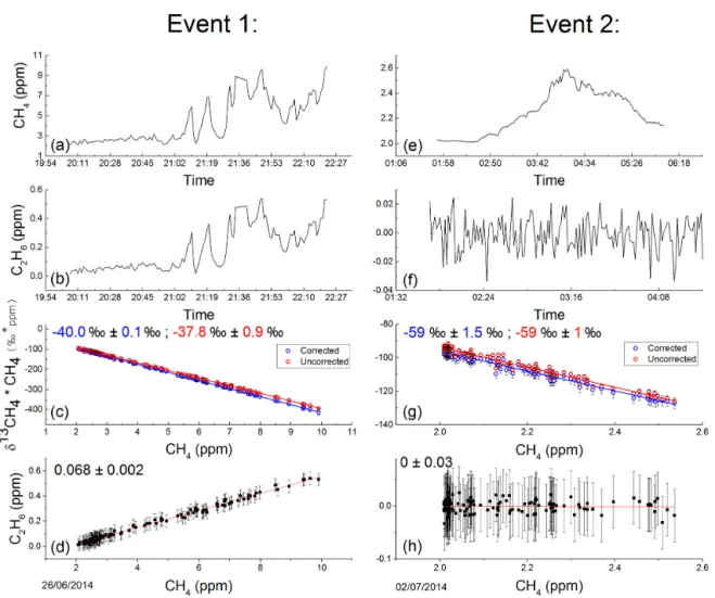
char-Figure 10. Ethane and methane content of two selected peaks. Methane and ethane 1 min averaged time series is shown in (a) and (b) for Event 1 and (e) and (f) for Event 2. Miller–Tans plots of the corresponding peaks are shown in (c) and (g), blue for the corrected δ13CH4 due to C2H6, and red representing uncorrected δ13CH4. Event 1 includes elevated C2H6emissions and thus displays a difference between the slope before and after C2H6correction, corresponding to a shift in isotopic signature. Event 2, with no C2H6shows no alteration in slope. The slopes of C2H6vs. CH4are shown in (d) and (h), signifying the C2H6: CH4ratio of the emission. Errors of both the isotopic and C2H6: CH4signatures are calculated from the standard error of the slope.
acterized using the Miller–Tans method (Miller and Tans, 2003), in which δ13CH∗4CH4values are plotted against CH4
to calculate the isotopic signature of the methane source in situations where the background is not constant. In order to avoid bias stemming from using ordinary least squared (OLS) regression, the York least squares fitting method was implemented, thus taking into account both the X and Y er-rors (York, 1968). All events excluding one were found to have δ13CH4 signatures characteristic of natural gas,
cor-responding on average to −40 ‰. A single event (Event 2 plotted in Fig. 10) was detected with a δ13CH4signature of
−59 ‰ ± 1.5 ‰. Such a signature suggests a biogenic source and, due to the south-westerly wind direction throughout the event (where the livestock holding is located), suggests the source is likely to originate from livestock, either as rumi-nant or manure emissions.
If the data are left uncorrected, sources containing C2H6
substantially bias the calculated isotopic signature of CH4
events. This is demonstrated in Fig. 10c where, for Event 1, the slope of points after C2H6correction (in blue) is shifted in
comparison to the slope derived from points left uncorrected (in red), signifying a modification of the δ13CH4 signature.
Corrected δ13CH4suggests a signature of −40.0 ‰ ± 0.1 ‰,
while uncorrected values imply −37.8 ‰ ± 0.08 ‰. When no C2H6 is present, i.e. Event 2, there is no disparity
be-tween the raw and corrected δ13CH4 slope, resulting in a
δ13CH4 signature of −59 ‰ ± 1 ‰ for both methods. For
the 15 natural-gas-related events, the average shift induced due to uncorrected data is 2 ‰. Consequently the bias in iso-topic signatures due to C2H6 means that uncorrected data
will always overestimate the source when a simple two end-member mixing model is applied.
4.3 Continuous field measurements of ethane
As an independent verification of the CRDS performance we compared two time series of C2H6which were measured
si-multaneously by the CRDS and GC-FID during the natural gas field campaign by using a co-located air inlet. The CRDS data were averaged to identical time stamps as the GC-FID, i.e. a 10 min average every 30 min. From which we calculated a root mean squared error (RMSE) of 13 ppb. Given the pre-cision of C2H6measured by the CRDS instrument is 10 ppb
for 10 min averages, and the uncertainty on the GC-FID is 15 %, we conclude that this is an extremely good agreement. Furthermore, the flask samples, taken on the 4 July 2014, were measured by the CRDS to have a C2H6: CH4ratio of
0.074 ± 0.001 ppm C2H6/ppm CH4and 0.046 ± 0.003 ppm
C2H6/ppm CH4for the gas within Pipeline 1 and Pipeline
2 respectively. On the same day gas quality data from the on-site GC recorded a C2H6: CH4 ratio of 0.075 ppm
C2H6/ppm CH4 and 0.048 ppm C2H6/ppm CH4
respec-tively. Although the error associated with the later figures is unknown, the strong agreement between the two verifies our correction and calibration strategy of C2H6.
4.4 Use of continuous observations of C2H6: CH4by
CRDS
The instruments’ capability to now measure interference-corrected and calibrated C2H6 opens the door for
us-ing another proxy for source apportionment, namely the C2H6: CH4 ratio (Yacovitch et al., 2014, Roscioli et al.,
2015, Smith et al., 2015). The C2H6: CH4ratio that
charac-terizes each source is determined by the slope of the C2H6to
CH4relationship. This method was applied to the 16 events
identified within the natural gas field campaign, again us-ing the York linear regression method, takus-ing into account both X and Y error. Two examples of this method are dis-played in the bottom panel of Fig. 10. Event 1, represent-ing a natural gas emission has a measured C2H6: CH4
ra-tio of 0.068 ± 0.002 ppm C2H6/ppm CH4, suggesting a wet
gas source. Biogenic events, such as Event 2, are absent of C2H6 (within our detection limit), thus resulting in a
C2H6: CH4ratio of 0 ± 0.2 ppm C2H6/ppm CH4.
Exclud-ing the biogenic event, on average the 15 natural gas emis-sions detected have a weighted mean C2H6: CH4 ratio of
0.069 ppm C2H6/ppm CH4 with an average event
uncer-tainty of 0.006 ppm C2H6/ppm CH4. This figure agrees well
with the median value for conventional gas ratios measured by Roscioli et al. (2015).
If the C2H6data are left uncorrected and uncalibrated the
C2H6: CH4 ratio calculated is significantly shifted by
ap-proximately +0.06. The average raw C2H6: CH4 ratio for
the 15 natural gas events is 0.132 ± 0.007 ppm C2H6/ppm
CH4, while the biogenic events C2H6: CH4ratio calculated
is negative and thus impossible.
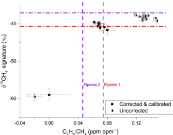
Figure 11. Distribution of 16 events according to their C2H6: CH4 ratios and isotopic signature. The red and purple dashed lines sig-nify the characterizations of Pipeline 1 and 2 respectively as mea-sured by the CRDS instrument from flask samples taken on the 4 July 14. For corrected and calibrated data (square markers), both the isotopic signature and C2H6: CH4ratios identify the biogenic source (bottom-left point) and suggest the natural gas emissions em-anate from Pipeline 1. Circular markers represent the uncorrected data which does not agree with the flask sample measurements of pipelines 1 or 2. The error bars indicate the standard error of the slope calculated from Miller–Tans and C2H6vs. CH4plots for δ13CH4signature and C2H6: CH4ratio respectively.
Figure 12. Flow chart illustrating the steps and the correspond-ing equations to calibrate C2H6and δ13CH4 as determined from this study. The coefficients are the mean of both CRDS instruments tested. We suggest removing H2O from gas samples prior to analy-sis.
4.5 Combined method for CH4source apportionment
To distinguish which pipeline the emissions originate from, we compare both the δ13CH4signature and the C2H6: CH4
ratio source apportionment methods. The two pipelines were characterized from the whole-air samples taken on 4 July 2014; although the gas within the pipelines is subject to change as incoming gas varies, we assume here that this did not occur throughout the short duration of the campaign (24 June to 4 July 2014). The data collected from the aforemen-tioned 16 events are compiled within Fig. 11, which illus-trates the distribution of δ13CH4 signature vs. C2H6: CH4
ratios. The results from the flask measurements, i.e. char-acteristics of Pipeline 1 and 2, are plotted as dashed pur-ple and red lines. Both methods clearly identify the bio-genic source, seen as an outlier in the bottom left corner of the plot. Furthermore, both methods are able to distin-guish between the two pipelines. The isotopic signatures of the natural gas events (on average 40.2 ‰ ± 0.5 ‰) are clustered near the isotopic signature of Pipeline 1, which has a δ13CH4signature of 40.7 ‰ ± 0.2 ‰, thus suggesting
the majority of the measured methane is an emission from this pipeline. When considering the C2H6: CH4ratio a
sim-ilar conclusion may be drawn as the mean C2H6: CH4
ra-tio is 0.069 ± 0.002 ppm C2H6/ppm CH4, much like that of
Pipeline 1 at 0.074 ± 0.003. A future study will address the shift in measured events to the left of Pipeline 1 in Fig. 11 by using additional VOC data from the GC-FID to aid source identification. The uncorrected 16 events are also plotted in Fig. 11 as circular markers. These are found in the top right-hand corner of Fig. 11 and do not correspond well with either of the pipelines, thus reconfirming the importance of the cor-rections.
5 Concluding remarks
This study focuses on measurements of C2H6contaminated
methane sources by a CRDS (Picarro G2201-i), with empha-sis on correcting δ13CH4and (although not intended for use
by standard users) C2H6 for cross-interferences before
cal-ibration. Our extensive laboratory tests suggest that CRDS instruments of this model are all subject to similar interfer-ences (as expected as they scan the same spectral lines) and that they can have a significant impact on reported concen-trations and isotopic signatures if not accounted for properly when measuring industrial natural gas sources. For now, we suggest using constant, instrument-specific correction factors if possible or the ones found in this study (summarized in Fig. 12). As our study period only encompasses 1 year it is clear that the stability of the correction over the full life-time needs to be monitored further. To fully exploit the reported C2H6data, we suggest drying gas samples to < 0.16 % H2O,
calibrating the instrument and taking frequent measurements of a working gas (or set of working gases) to monitor and correct for the instrumental baseline drift.
The results of our field campaign demonstrate the extent of the interferences of C2H6on δ13CH4for a real world
applica-tion and also support the validity of our C2H6correction and
calibration through the comparison with an independently calibrated GC-FID. In our case, when measuring wet gas emissions we detected an average shift in isotopic signature of 2.5 ‰ due to C2H6interference; however the extent of this
bias will vary according to the contribution of C2H6,
there-fore affecting each ffCH4source to a different degree which
can cause problems for source determination. The results re-ported here are important for all future work of CRDS in
fos-sil fuel regions (where sources consist of a C2H6: CH4ratio
between 0 and 1 ppm C2H6/ppm CH4)to create awareness
of such interferences and correct for them accordingly. Our CRDS instrument is sufficient for measurements of strongly variable C2H6sources, where if using calibrated 1 min C2H6
data, concentration variations above 150 ppb are required to achieve a signal-to-noise ratio of 5. Thus for industrial nat-ural gas sites it offers a new opportunity to use continuous C2H6: CH4 observations as a means of source
determina-tion that is independent from δ13CH4methods. The recently
released G2210-i analyser is dedicated to C2H6: CH4 ratio
measurements and as such achieves a higher precision, mak-ing it suitable for a wider variety of ethane sources.
Finally, we successfully combined both the δ13CH4 and
C2H6: CH4ratio source apportionment methods. At the
nat-ural gas compressor site both methods clearly distinguish biogenic sources from that of natural-gas-based sources. Combining those two independent methods yields a better fingerprint of the source and spurious C2H6or δ13CH4can
be more easily identified. Lastly, by characterizing both the δ13CH4and C2H6: CH4ratio of our source, we gain insight
into the formation and source region of the gas (Schoell, 1983).
Code and data availability. Code and data are available on request.
The Supplement related to this article is available online at https://doi.org/10.5194/amt-10-2077-2017-supplement.
Competing interests. The authors declare that they have no conflict of interest.
Acknowledgements. The authors would like to thank the NPL team for organizing the field campaign, in particular the support from Rod Robinson, Fabrizio Innocenti and Andrew Finlayson. We thank our LSCE colleagues: Camille Yver Kwok and Se-bastien Ars for assistance during the field campaign, as well as Bernard Bonsang and Dominique Basinee for their technical help and contributions on the GC instruments both on and off the field. We also thank Rebecca Fisher (RHUL) and Dave Lowry for their contributions, especially for measurements of δ13CH4 for our calibration cylinders under the InGOS’ TransNational Access programme (TNA-id-666; http://www.ingos-infrastructure.eu/ project-info/workpackages/tna-transnational-access/). This work was supported by the Climate KIC through the FuME project (http://www.climate-kic.org/projects/fume/) and the funding of the PhD studies of Sabina Assan through the education of climate KIC. Edited by: M. Hamilton
References
Allen, D. T.: Methane emissions from natural gas production and use: reconciling bottom-up and top-down measurements, Current Opinion in Chemical Engineering, 5, 78–83, 2014.
Bonsang, B. and Kanakidou, M.: Nonmethane hydrocarbon mea-surements during the FIELDVOC 1994 experiment, Chemo-sphere, Global Change Science, 3, 259–273, 2001.
Fisher, R., Lowry, D., Wilkin, O., Sriskantharajah, S.. and Nis-bet, G.: High- precision, automated stable isotope analysis of atmospheric methane and carbon dioxide using continuous-flow isotope-ratio mass spectrometery, Rapid Commun. Mass Spec-trom., 20, 200–208, 2006.
Gilman, J. B., Lerner, B. M., Kuster, W. C., and De Gouw, J. A.: Source signature of volatile organic compounds from oil and nat-ural gas operations in northeastern Colorado, Environ. Sci. Tech-nol., 47, 1297–1305, 2013.
Gros, V. , Gaimoz, C., Herrmann, F., Custer, T., Williams, J., Bon-sang, B., Sauvage, S., Locoge, N., d’Argouges, O., Sarda-Estève, R., and Sciare, J.: Volatile Organic Compounds Sources in Paris in spring 2007. Part I: qualitative analysis, Environ. Chem., 8, 74–90, 2011.
Hiller, R. V., Bretscher, D., DelSontro, T., Diem, T., Eugster, W., Henneberger, R., Hobi, S., Hodson, E., Imer, D., Kreuzer, M., Künzle, T., Merbold, L., Niklaus, P. A., Rihm, B., Schel-lenberger, A., Schroth, M. H., Schubert, C. J., Siegrist, H., Stieger, J., Buchmann, N., and Brunner, D.: Anthropogenic and natural methane fluxes in Switzerland synthesized within a spatially explicit inventory, Biogeosciences, 11, 1941–1959, https://doi.org/10.5194/bg-11-1941-2014, 2014.
Höglund-Isaksson, L.: Global anthropogenic methane emissions 2005–2030: technical mitigation potentials and costs, Atmos. Chem. Phys., 12, 9079–9096, https://doi.org/10.5194/acp-12-9079-2012, 2012.
Jackson, R. B., Down, A., Phillips, N. G., Ackley, R. C., Cook, C. W., Plata, D. L., and Zhao, K.: Natural gas pipeline leaks across Washington, DC, Environ. Sci. Technol., 48, 2051–2058, 2014. Kirschke, S., Bousquet, P., Ciais, P., Saunois, M., Canadell, J. G.,
Dlugokencky, E., Bergamaschi, P., Bergmann, D., Blake, D., Bruhwiler, L., Cameron-Smith, P., Castaldi, S., Chevallier, F., Feng, L., Fraser, A., Heimann, M., Hodson, E., Houweling, S., Josse, B., Fraser, P. J., Krummel, P. B., Lamarque, J., Langen-felds, R. L., Le Quéré, C., Naik, V., O’Doherty, S., Palmer, P. I., Pison, I., Plummer, D., Poulter, B., Prinn, R. J., Rigby, M., Ringeval, B., Santini, M., Schmidt, M., Shindell, D. T., Simpson, I. J. Spahni, R., Steele, l. P., Strode, S. A., Sudo, K., Szopa, S., van der Werf, G. R., Voulgarakis, A., van Weele, M., Weiss, R. F., Williams, J. E., and Zeng, G.: Three decades of global methane sources and sinks, Nat. Geosci., 6, 813-823, 2013.
Lamb, B. K., McManus, J. B., Shorter, J. H., Kolb, C. E., Mosher, B., Harriss, R. C., Allwine, E., Blaha, D., Howard,T ., Guenther, A., Lott, R. A., Siverson, R., Westburg, H., and Zimmerman, P.: Development of atmospheric tracer methods to measure methane emissions from natural gas facilities and urban areas, Environ. Sci. Technol., 29, 1468–1479, 1995.
Laurent, O. et al.: Icos ATC Metrology Lab: Metrological perfor-mance assessment of GHG analyzers, Atmospheric Measure-ment Techniques 8.10 4075–4082, Poster session presented at: 18th WMO/IAWA Meeting on Carbon Dioxide, Other
Green-house Gases, and Related Measurement Techniques (GGMT), 13–17 September, California, CA, 2015.
Lowry, D., Holmes, C. W., Rata, N. D., O’Brien, P., and Nisbet, E. G.: London methane emissions: Use of diurnal changes in con-centration and δ13C to identify urban sources and verify inven-tories, J. Geophys. Res.-Atmos., 106, 7427–7448, 2001. Malowany, K., Stix, J., Van Pelt, A., and Lucic, G.: H2S
interfer-ence on CO2 isotopic measurements using a Picarro G1101-i cavity ring-down spectrometer, Atmos. Meas. Tech., 8, 4075– 4082, https://doi.org/10.5194/amt-8-4075-2015, 2015.
Miller, J. B. and Tans, P. P.: Calculating isotopic fractionation from atmospheric measurements at various scales, Tellus B, 55.2, 207– 214, 2003.
Nara, H., Tanimoto, H., Tohjima, Y., Mukai, H., Nojiri, Y., Katsumata, K., and Rella, C. W.: Effect of air composition (N2, O2, Ar, and H2O) on CO2 and CH4 measurement by wavelength-scanned cavity ring–down spectroscopy: calibration and measurement strategy, Atmos. Meas. Tech., 5, 2689–2701, https://doi.org/10.5194/amt-5-2689-2012, 2012.
Phillips, N. G., Ackley, R., Crosson, E. R., Down, A., Hutyra, L. R., Brondfield, M., Karr, J. D., Zhao, K., and Jackson, R. B.: Map-ping urban pipeline leaks: Methane leaks across Boston, Environ. Pollut., 173, 1–4, 2013.
Rella, C. W., Hoffnagle, J., He, Y., and Tajima, S.: Local- and regional-scale measurements of CH4, δ13CH4, and C2H6in the Uintah Basin using a mobile stable isotope analyzer, Atmos. Meas. Tech., 8, 4539–4559, https://doi.org/10.5194/amt-8-4539-2015, 2015.
Roscioli, J. R., Yacovitch, T. I., Floerchinger, C., Mitchell, A. L., Tkacik, D. S., Subramanian, R., Martinez, D. M., Vaughn, T. L., Williams, L., Zimmerle, D., Robinson, A. L., Hern-don, S. C., and Marchese, A. J.: Measurements of methane emissions from natural gas gathering facilities and processing plants: measurement methods, Atmos. Meas. Tech., 8, 2017– 2035, https://doi.org/10.5194/amt-8-2017-2015, 2015.
Schoell, M.: Genetic characterization of natural gases, AAPG bul-letin, 67, 2225–2238, 1983.
Smith, M. L., Kort, E. A., Karion, A., Sweeney, C., Herndon, S. C., and Yacovitch, T. I.: Airborne ethane observations in the Barnett shale: Quantification of ethane flux and attribution of methane emissions, Environ. Sci. Technol., 49, 8158–8166, 2015. Stevens, C. M. and Engelkemeir, A.: Stable carbon isotopic
compo-sition of methane from some natural and anthropogenic sources, J. Geophys. Res.-Atmos., 93, 725–733, 1988.
Subramanian, R., Williams, L. L., Vaughn, T. L., Zimmerle, D., Roscioli, J. R., Herndon, S. C., Yacovitch, T. L., Floerchinger, C., Tkacik, D. S., Mitchell, A. L., Sullivan, M. R., Dallmann, T. R., and Robinson, A. L.: Methane emissions from natural gas com-pressor stations in the transmission and storage sector: Measure-ments and comparisons with the EPA greenhouse gas reporting program protocol, Environ. Sci. Technol., 49, 3252–3261, 2015. US Environmental Protection Agency: Inventory of U.S Greenhouse Gas Emissions and Sinks: 1990– 2014, EPA 430-R-16-002, Annex 7, available at: https://www3.epa.gov/climatechange/Downloads/ghgemissions/ US-GHG-Inventory-2016-Annex-7-Uncertainty.pdf (last access: 2 May 2017), 2016.
Vogel, F. R., Huang, L., Ernst, D., Giroux, L., Racki, S., and Worthy, D. E. J.: Evaluation of a cavity ring-down spectrometer for in
situ observations of 13CO2, Atmos. Meas. Tech., 6, 301–308, https://doi.org/10.5194/amt-6-301-2013, 2013.
Yacovitch, T. I., Herndon, S. C., Roscioli, J. R., Floerchinger, C., McGovern, R. M., Agnese, M., Pétron, G., Kofler, J., Sweeney, C., Karion, A., Conley, S. A., Kort, E. A., Nähle,L., Fischer, M., Hildebrandt,L., Koeth,J., McManus, J. B., Nelson, D. D., Zah-niser, M. S., and Kolb, C. E.: Demonstration of an ethane spec-trometer for methane source identification, Environ. Sci. Tech-nol., 48, 8028–8034, 2014.
Yacovitch, T. I., Herndon, S. C., Pétron, G., Kofler, J., Lyon, D., Zahniser, M. S., and Kolb, C. E.: Mobile laboratory observations of methane emissions in the Barnett Shale region, Environ. Sci. Technol., 49, 7889–7895, 2015.
York, D.: Least squares fitting of a straight line with correlated er-rors, Earth Planet. Sc. Lett., 5, 320–324, 1968.
Yvon-Lewis, S. A., Hu, L., and Kessler, J.: Methane flux to the atmosphere from the Deepwater Horizon oil disaster, Geophys. Res. Lett., 38, L01602, https://doi.org/10.1029/2010GL045928, 2011.