Disentangled Representations in Neural Models
by
William Whitney
S.B., Massachusetts Institute of Technology (2013)
Submitted to the Department of Electrical Engineering and Computer
Science
in partial fulfillment of the requirements for the degree of
Master of Engineering in Computer Science and Engineering
at the
MASSACHUSETTS INSTITUTE OF TECHNOLOGY
February 2016
© William Whitney, MMXVI. All rights reserved.
The author hereby grants to MIT permission to reproduce and to
distribute publicly paper and electronic copies of this thesis document
in whole or in part in any medium now known or hereafter created.
Author . . . .
Department of Electrical Engineering and Computer Science
January 29, 2016
Certified by. . . .
Joshua B. Tenenbaum
Professor
Thesis Supervisor
Accepted by . . . .
Christopher Terman
Chairman, Masters of Engineering Thesis Committee
Disentangled Representations in Neural Models
by
William Whitney
Submitted to the Department of Electrical Engineering and Computer Science on January 29, 2016, in partial fulfillment of the
requirements for the degree of
Master of Engineering in Computer Science and Engineering
Abstract
Representation learning is the foundation for the recent success of neural network models. However, the distributed representations generated by neural networks are far from ideal. Due to their highly entangled nature, they are difficult to reuse and interpret, and they do a poor job of capturing the sparsity which is present in real-world transformations.
In this paper, I describe methods for learning disentangled representations in the two domains of graphics and computation. These methods allow neural methods to learn representations which are easy to interpret and reuse, yet they incur little or no penalty to performance. In the Graphics section, I demonstrate the ability of these methods to infer the generating parameters of images and rerender those images under novel conditions. In the Computation section, I describe a model which is able to factorize a multitask learning problem into subtasks and which experiences no catastrophic forgetting. Together these techniques provide the tools to design a wide range of models that learn disentangled representations and better model the factors of variation in the real world.
Thesis Supervisor: Joshua B. Tenenbaum Title: Professor
Acknowledgments
I would like to thank my girlfriend, Benjana, who is my joy. She lets me see my work through new eyes.
I thank Tejas Kulkarni for his mentorship and friendship. He has been my gateway into this world and a strong guiding influence, and I would not be here without him. I thank Josh Tenenbaum for his guidance. He has pushed me to think about the most fundamental problems.
I thank my parents for their constant love and support. They made me this way, so please direct all complaints to them.
I thank Thomas Vetter for access to the Basel face model. I am grateful for support from the MIT Center for Brains, Minds, and Machines (CBMM).
Contents
1 Introduction 12
1.1 Document overview . . . 13
2 Desiderata for representations 14 2.1 Disentangled . . . 14 2.2 Interpretable . . . 15 2.3 Performant . . . 16 2.4 Reusable . . . 16 2.5 Compact . . . 17 3 Disentanglement in Vision 18 3.1 Introduction . . . 18 3.2 Related Work . . . 20 3.3 Model . . . 22
3.3.1 Training with Specific Transformations . . . 24
3.3.2 Invariance Targeting . . . 27
3.4 Experiments . . . 27
3.4.1 3D Face Dataset . . . 30
3.4.2 Comparison with Entangled Representations . . . 31
3.4.3 Chair Dataset . . . 33
4 Disentanglement in Computation 36 4.1 Introduction . . . 36
4.1.1 Catastrophic forgetting . . . 40
4.2 Related Work . . . 41
4.3 Controller-function networks . . . 42
4.3.1 Relationship to mixture of experts . . . 44
4.3.2 Hard and soft decisions . . . 44
4.3.3 Continuation methods . . . 45
4.3.4 Training with noisy decisions . . . 46
4.4 Experiments . . . 47 4.4.1 Disentanglement of functions . . . 48 4.4.2 Catastrophic forgetting . . . 50 5 Discussion 52 5.1 DC-IGN . . . 52 5.1.1 Future work . . . 53 5.2 Controller-function networks . . . 53 5.2.1 Future work . . . 54 5.3 Unification . . . 56 References 57
List of Figures
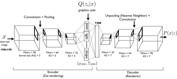
3-1 Model Architecture. Deep Convolutional Inverse Graphics Net-work (DC-IGN) has an encoder and a decoder. We follow the varia-tional autoencoder (Kingma and Welling 2013) architecture with vari-ations. The encoder consists of several layers of convolutions followed by max-pooling and the decoder has several layers of unpooling (up-sampling using nearest neighbors) followed by convolution. (a) During training, data 𝑥 is passed through the encoder to produce the pos-terior approximation 𝑄(𝑧𝑖|𝑥), where 𝑧𝑖 consists of scene latent
vari-ables such as pose, light, texture or shape. In order to learn pa-rameters in DC-IGN, gradients are back-propagated using stochas-tic gradient descent using the following variational object function: −𝑙𝑜𝑔(𝑃 (𝑥|𝑧𝑖)) + 𝐾𝐿(𝑄(𝑧𝑖|𝑥)||𝑃 (𝑧𝑖)) for every 𝑧𝑖. We can force
DC-IGN to learn a disentangled representation by showing mini-batches with a set of inactive and active transformations (e.g. face rotating, light sweeping in some direction etc). (b) During test, data 𝑥 can be passed through the encoder to get latents 𝑧𝑖. Images can be
re-rendered to different viewpoints, lighting conditions, shape variations, etc by setting the appropriate graphics code group (𝑧𝑖), which is how
one would manipulate an off-the-shelf 3D graphics engine. . . 23 3-2 Structure of the representation vector. 𝜑 is the azimuth of the
face, 𝛼 is the elevation of the face with respect to the camera, and 𝜑𝐿
3-3 Training on a minibatch in which only 𝜑, the azimuth angle of the face, changes. During the forward step, the output from each component 𝑧𝑖 ̸= 𝑧1 of the encoder is altered to be the same for each
sample in the batch. This reflects the fact that the generating variables of the image (e.g. the identity of the face) which correspond to the desired values of these latents are unchanged throughout the batch. By holding these outputs constant throughout the batch, the single neuron 𝑧1 is forced to explain all the variance within the batch, i.e. the
full range of changes to the image caused by changing 𝜑. During the backward step 𝑧1 is the only neuron which receives a gradient signal
from the attempted reconstruction, and all 𝑧𝑖 ̸= 𝑧1 receive a signal
which nudges them to be closer to their respective averages over the batch. During the complete training process, after this batch, another batch is selected at random; it likewise contains variations of only one of 𝜑, 𝛼, 𝜑𝐿, 𝑖𝑛𝑡𝑟𝑖𝑛𝑠𝑖𝑐; all neurons which do not correspond to the selected
latent are clamped; and the training proceeds. . . 25 3-4 Manipulating light. Qualitative results showing the generalization
capability of the learned DC-IGN decoder to re-render a single input image under different lighting conditions. We change the latent 𝑧𝑙𝑖𝑔ℎ𝑡
smoothly leaving all 199 other latents unchanged. . . 28 3-5 Manipulating elevation. Results showing the ability of the
DC-IGN decoder to change the elevation of the input image. We change the latent 𝑧𝑒𝑙𝑒𝑣𝑎𝑡𝑖𝑜𝑛 smoothly leaving all 199 other latents unchanged. 29
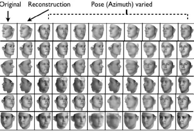
3-6 Manipulating azimuth (horizontal angle). Qualitative results showing the generalization capability of the learnt DC-IGN decoder to render original static image with different azimuth (pose) directions. The latent neuron 𝑧𝑎𝑧𝑖𝑚𝑢𝑡ℎ is changed to random values but all other
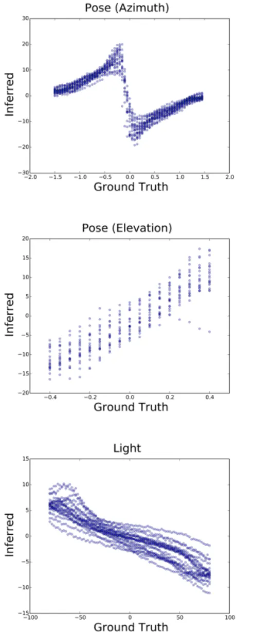
3-7 Generalization of decoder to render images in novel view-points and lighting conditions. We generated several datasets by varying light, azimuth and elevation, and tested the invariance proper-ties of DC-IGN’s representation 𝑍. We show quantitative performance on three network configurations as described in Sec. 3.4.1. All DC-IGN encoder networks reasonably predicts transformations from static test images. Interestingly, as seen in the first plot, the encoder net-work seems to have learnt a switch node to deal uniquely with the mirror-symmetric sides of the face. . . 32
3-8 Entangled versus disentangled representations. First column: Original images. Second column: transformed image using DC-IGN. Third column: transformed image using normally-trained network. . . 33
3-9 Manipulating rotation: Each row was generated by encoding the input image (leftmost) with the encoder, then changing the value of a single latent and putting this modified encoding through the decoder. The network has never seen these chairs before at any orientation. Top: Some positive examples. Note that the DC-IGN is making a conjecture about any components of the chair it cannot see; in par-ticular, it guesses that the chair in the top row has arms, because it can’t see that it doesn’t. Bottom: Examples in which the network extrapolates to new viewpoints less accurately. . . 34
4-1 The controller and layers of the CFN. The controller provides weights on each layer as a function of the data. This shows three layers, but there can be many more. . . 42
4-2 Disentanglement and validation loss plotted over the course of training. Disentanglement, or independence, is measured by the L2 norm of the weight vector over the functions. In this measure, 0.35 is totally entangled, with every function accorded equal weight for every input, and 1.0 is totally disentangled, with precisely one function used for each input. Left: with sharpening and noise. Right: without sharpening and noise. . . 49 4-3 Forgetting when trained on one task. When a traditional
feed-forward network, which previously trained on several tasks, is trained exclusively on one, it forgets how to perform the others. The controller-function network is practically immune to forgetting. In this figure, we see each network trained exclusively on one of several tasks it is able to do. The loss that is shown is the average L2 error attained on all of the other tasks as this network retrains. . . 50 5-1 Multistep CFN. A variant of the design for using multiple timesteps
1. Introduction
Representation is one of the most fundamental problems in machine learning. It underlies such varied fields as vision, speech recognition, natural language process-ing, reinforcement learnprocess-ing, and graphics. Yet the question of what makes a good representation is a deceptively complex one. On the one hand, we would like repre-sentations which perform well on real-world tasks. On the other, we would like to be able to interpret these representations, and they should be useful for tasks beyond those explicit in their initial design.
Presently representations come in two varieties: those that are designed, and those that are learned from data. Designed representations can perfectly match our desire for structured reuse and interpretability, while learned representations require no expert knowledge yet outperform designed features on practically every task that has sufficient data.
This tension has been the source of great debate in the community. Clearly a rep-resentation which has some factorizable structure can be more readily reused in part or in whole for some new task. Much more than being just an issue of interpretation, this concern has a very practical focus on generalization; it is unreasonable to spend a tremendous amount of data building a new representation for every single task, even when those tasks have strong commonalities. Since we have knowledge about the true structure of the problem, we can design a representation which is factorized and thus reusable.
Learned representations take a very different approach to the problem. Instead of attempting to incorporate expert knowledge of a domain to create a representation which will be broadly useful, a learned representation is simply the solution to a single
optimization problem. It is custom-designed to solve precisely the task it was trained on, and while it may be possible to reverse-engineer such a representation for reuse elsewhere, it is typically unclear how to do so and how useful it will be in a secondary setting.
Despite the obvious advantages of structured representations, those we design are inherently limited by our understanding of the problem. Perhaps it is possible to design image features with spokes and circles that will be able to distinguish a bike wheel from a car wheel, but there are a million subtle clues that no human would think to include. As a result, in domain after domain, as the datasets have grown larger, representations learned by deep neural networks have come to dominate.
The dominance of optimization-based representation learning is unavoidable and in fact hugely beneficial to the field. However, the weaknesses of these learned repre-sentations is not inherent in their nature; it merely reflects the limits of our current tasks and techniques.
This thesis represents an effort to bring together the advantages of each of these techniques to learn representations which perform well, yet have valuable structure. Using the two domains of graphics and programs, I will discuss the rationale, tech-niques, and results of bringing structure to neural representations.
1.1
Document overview
The next chapter discusses various criteria for assessing the quality of a representation. In the following two chapters, I use these criteria to discuss representations in the domains of graphics and computer programs. Each chapter begins with an overview of the problems in the field and related work, then moves on to a description of the specific problem I address, my methods, and the results.
In the final chapter I discuss the significance of this work to the field and promising directions for further research.
2. Desiderata for representations
When evaluating a representation, it is valuable to have a clear set of goals. Several of the goals stated here have substantial overlap, and to some degree a representation which perfectly addresses one may automatically fulfill another as well. However, each of them provides a distinct benefit, and their significance must be considered with respect to those benefits.
2.1
Disentangled
A representation which is disentangled for a particular dataset is one which is sparse over the transformations present in that data (Bengio, Courville, and Vincent 2013). For example, given a dataset of indoor videos, a representation that explicitly rep-resents whether or not the lights are on is more disentangled than a representation composed of raw pixels. This is because for the common transformation of flipping the light switch, the first representation will only change in only that single dimension (light on or off), whereas the second will change in every single dimension (pixel).
For a representation to be disentangled implies that it factorizes some latent cause or causes of variation. If there are two causes for the transformations in the data which do not always happen together and which are distinguishable, a maximally disentangled representation will have a structure that separates those causes. In the indoor scenes example above, there might be two sources of lighting: sunlight and electric lights. Since transformations in each of these latent variables occur independently, it is more sparse to represent them separately.
expressing the “true” generative process for that data. In graphics this model might represent each object in a room, with its pose in the scene and its intrinsic reflectance characteristics, and the sources of lighting. For real-world transformations involving motion, only the pose of each object needs to be updated. As the lighting shifts, noth-ing about the representation of the objects needs to be changed; the visual appearance of the object can be recalculated from the new lighting variables.
In a certain light, all of science is one big unsupervised learning problem in which we search for the most disentangled representation of the world around us.
2.2
Interpretable
An interpretable representation is, simply enough, one that is easy for humans to understand. A human should be able to make predictions about what changes in the source domain would do in the representation domain and vice versa. In a graphics engine’s representation of a scene, for example, it is easy for a person to predict things like “What would the image (source domain) look like if I changed the angle of this chair (representation domain) by 90°?” By contrast, in the representation of a classically-trained autoencoder, it is practically impossible for a person to visualize the image that would be generated if some particular component were changed.
Interpretability is closely related with disentanglement. This is because, in “hu-man” domains of data like vision and audition, humans are remarkably good at in-ferring generative structure, and tend to internally use highly disentangled repre-sentations. However, this relationship only holds for datasets which are similar to human experience. One could construct a dataset of videos in which the most com-mon transformation between frames was for each pixel in the image to change its hue by an amount proportional to the number of characters in the Arabic name of the object shown in that pixel. The most disentangled representation of these videos would perfectly match this structure, but this disentangled representation would be less interpretable than a table of English names of objects and how much their color changes per frame.
In a real-world setting, the most disentangled possible representation of stock market prices might involve a latent which represents a complex agglomeration of public opinion from the news, consumer confidence ratings, and estimates of the Fed’s likelihood of raising rates. Such a latent might truly be the best and most independent axis of variation for predicting the stock price, yet it would not be as easy to interpret as a representation with one latent for public opinion, one latent for the Fed, and one latent for consumer confidence. In such a non-human domain, our intuitions about the factors of variation may not hold, and as a result the representations that make sense to us and those that accurately represent the factors of variation may diverge. Interpretability is extremely valuable in many domains. If a doctor is attempting to plan a course of treatment for a patient, they need to be able to reason about the factors in a diagnostic model they’re using. Even if an algorithm doesn’t need to in-terface with a human at runtime, it’s very hard to debug a system during development if you don’t understand what it’s doing.
2.3
Performant
A performant representation for a task contains the information needed to perform well on that task.
If the task is determining whether or not there is a dog in a room, a representation consisting of a photograph of the room would be less performant than a 3D voxel model of the room, which in turn would be less performant than a single binary bit representing whether or not there is a dog.
2.4
Reusable
A reusable representation is one that is performant for many tasks in the same domain. To continue the example above, a 3D voxel representation of a room is more reusable than one indicating whether or not the room contains a dog. Somewhere in between the two would be a representation consisting of the facts,
• Is there an animal? • Is it furry?
• How big is it? • What color is it?
This representation would be able to solve the task of whether or not the room contains a dog with high probability, and would also be able to inform the task of whether or not the room contains a gorilla, or a whale. However, the tasks it can address are a strict subset of the voxel representation, which could also solve such problems as “Where is the couch?”
2.5
Compact
A compact representation is one which occupies few bits.
Compactness may not seem inherently important; it is typically irrelevant if the representation of an image takes up one megabyte or two. However, compactness provides a very valuable forcing function. One might build a weather forecasting model which represents the state of the world down to the very last butterfly.
The actions of this butterfly might be indeterminate given the other latents in the model, so it is disentangled; it might be perfectly easy to understand the meaning of the butterfly’s representation, so it is interpretable; it might be valuable in some other system or context, so it is reusable; and it might even minutely improve the performance of the weather forecast, so it is performant. But somehow none of this quite justifies its presence in a weather model.
3. Disentanglement in Vision
3.1
Introduction
Deep learning has led to remarkable breakthroughs in learning hierarchical represen-tations from images. Models such as Convolutional Neural Networks (CNNs) (LeCun and Bengio 1995), Restricted Boltzmann Machines, (Hinton, Osindero, and Teh 2006, Salakhutdinov and Hinton (2009)), and Auto-encoders (Bengio 2009, Vincent et al. (2010)) have been successfully applied to produce multiple layers of increasingly ab-stract visual representations. However, there is relatively little work on characterizing the optimal representation of the data. While Cohen et al. (2014) have considered this problem by proposing a theoretical framework to learn irreducible representations with both invariances and equivariances, coming up with the best representation for any given task is an open question.
To shed some light on this question, let us consider our list of desires for repre-sentations in the specific context of vision.
1. Disentangled: When applied to real-world transformations over images, i.e. video, a good representation will change only sparsely. That is, the expectation over a set of videos of the number of dimensions of the representation which change between each frame should be small. In practice this means that common trans-formations, like movement of an object, should be expressed concisely; whereas uncommon transformations, like a solid object turning inside out, may be more expensive to express.
well with the one that’s in our heads. It should express objects separately from their conditions, and common transformations should be monotonic and smooth in representation space.
3. Performant: Representations of visual content need to be quite rich; in order to be able to solve problems like “Which of these objects is in front of the other?” a representation must understand much more than just pixels.
4. Reusable: A representation which was learned to solve a very specific task, like perhaps that of the DQN (Mnih et al. 2015), will not be helpful in other settings, like the real world. To be reusable a model needs to capture the structure that is universal to our world.
5. Compact: Representations of images should be able to efficiently compress the images in their domain.
The “vision as inverse graphics” paradigm suggests a representation for images which provides these features. Computer graphics consists of a function to go from compact descriptions of scenes (the graphics code) to images, and this graphics code is typically disentangled to allow for rendering scenes with fine-grained control over transformations such as object location, pose, lighting, texture, and shape. This en-coding is designed to easily and interpretably represent sequences of real data so that common transformations may be compactly represented in software code; this cri-terion is conceptually identical to disentanglement, and graphics codes conveniently align with the properties of an ideal representation. Graphics codes are the represen-tations which we as a society have designed to be the single most general-purpose, interpretable, and generally usable way to express scenes.
Early work by Tenenbaum et al. (2000) was among the first to explore this idea, and used bilinear models to differentiate between extrinsic and intrinsic factors in images. Recent work in inverse graphics (Mansinghka et al. 2013, Kulkarni et al. (2014), Kulkarni, Kohli, et al. (2015)) follows a general strategy of defining a probabilistic with latent parameters, then using an inference algorithm to find the
most appropriate set of latent parameters given the observations. Tieleman et al. (2014) moved beyond this two-stage pipeline by using a generic encoder network and a domain-specific decoder network to approximate a 2D rendering function. However, none of these approaches have been shown to automatically produce a semantically-interpretable graphics code and to learn a 3D rendering engine to reproduce images. I present an approach, first described in (Kulkarni, Whitney, et al. 2015), which attempts to learn interpretable graphics codes for complex transformations such as out-of-plane rotations and lighting variations. Given a set of images, we use a hybrid encoder-decoder model to learn a representation that is disentangled with respect to various transformations such as object out-of-plane rotations and lighting variations. We employ a deep directed graphical model with many layers of convolution and de-convolution operators that is trained using the Stochastic Gradient Variational Bayes (SGVB) algorithm (Kingma and Welling 2013).
We propose a training procedure to encourage each group of neurons in the graph-ics code layer to distinctly represent a specific transformation. To learn a disentangled representation, we train using data where each mini-batch has a set of active and in-active transformations, but we do not provide target values as in supervised learning; the objective function remains reconstruction quality. For example, a nodding face would have the 3D elevation transformation active but its shape, texture and other transformations would be inactive. We exploit this type of training data to force cho-sen neurons in the graphics code layer to specifically reprecho-sent active transformations, thereby automatically creating a disentangled representation. Given a single face im-age, our model can re-generate the input image with a different pose and lighting. We present qualitative and quantitative results of the model’s efficacy at learning a 3D rendering engine.
3.2
Related Work
As mentioned previously, a number of generative models have been proposed in the literature to obtain abstract visual representations. Unlike most RBM-based
mod-els (Hinton, Osindero, and Teh 2006, Salakhutdinov and Hinton (2009), Lee et al. (2009)), our approach is trained using back-propagation with objective function con-sisting of data reconstruction and the variational bound.
Relatively recently, Kingma et al. (Kingma and Welling 2013) proposed the SGVB algorithm to learn generative models with continuous latent variables. In this work, a feed-forward neural network (encoder) is used to approximate the posterior distribu-tion and a decoder network serves to enable stochastic reconstrucdistribu-tion of observadistribu-tions. In order to handle fine-grained geometry of faces, we work with relatively large scale images (150 × 150 pixels). Our approach extends and applies the SGVB algorithm to jointly train and utilize many layers of convolution and de-convolution operators for the encoder and decoder network respectively. The decoder network is a function that transform a compact graphics code (200 dimensions) to a 150 × 150 image. We pro-pose using unpooling (nearest neighbor sampling) followed by convolution to handle the massive increase in dimensionality with a manageable number of parameters.
(Dosovitskiy, Springenberg, and Brox 2015) proposed using CNNs to generate images given object-specific parameters in a supervised setting. As their approach requires ground-truth labels for the graphics code layer, it cannot be directly applied to image interpretation tasks. Our work is similar to Ranzato et al. (2007), whose work was amongst the first to use a generic encoder-decoder architecture for feature learning. However, in comparison to our proposal their model was trained layer-wise, the intermediate representations were not disentangled like a graphics code, and their approach does not use the variational auto-encoder loss to approximate the posterior distribution. Our work is also similar in spirit to (Tang, Salakhutdinov, and Hinton 2012), but in comparison our model does not assume a Lambertian reflectance model and implicitly constructs the 3D representations. Another piece of related work is Desjardins et al. (2012), who used a spike and slab prior to factorize representations in a generative deep network.
Quite recently, (Jaderberg et al. 2015) proposes a model which explicitly captures the pose of objects in a scene through the use of predefined 2D affine transforma-tions, which leads pose and identity to be disentangled. (Mansimov et al. 2015) use
an attention mechanism to generate images from text; this approach has the potential to learn functions which are parametrized by highly disentangled symbolic represen-tations. (Theis and Bethge 2015) use spatial LSTMs to build generative models of textures in natural images.
In comparison to prior approaches, it is important to note that our encoder net-work produces the interpretable and disentangled representations necessary to learn a meaningful 3D graphics engine. A number of inverse-graphics inspired methods have recently been proposed in the literature (Mansinghka et al. 2013). However, most such methods rely on hand-crafted rendering engines. The exception to this is work by Hinton et al. (2011) and Tieleman (2014) on transforming autoencoders which use a domain-specific decoder to reconstruct input images.
(Yang et al. 2015) follows up on our work with a recurrent model which learns similar disentangled representations from watching synthesized video.
3.3
Model
As shown in Figure fig. 3-1, the basic structure of the Deep Convolutional Inverse Graphics Network (DC-IGN) consists of two parts: an encoder network which cap-tures a distribution over graphics codes 𝑍 given data 𝑥 and a decoder network which learns a conditional distribution to produce an approximation ˆ𝑥 given 𝑍. 𝑍 can be a disentangled representation containing a factored set of latent variables 𝑧𝑖 ∈ 𝑍 such
as pose, light and shape. This is important in learning a meaningful approximation of a 3D graphics engine and helps tease apart the generalization capability of the model with respect to different types of transformations.
Let us denote the encoder output of DC-IGN to be 𝑦𝑒 = 𝑒𝑛𝑐𝑜𝑑𝑒𝑟(𝑥). The encoder
output is used to parametrize the variational approximation 𝑄(𝑧𝑖|𝑦𝑒), where 𝑄 is
chosen to be a multivariate normal distribution. There are two reasons for using this parametrization:
1. Gradients of samples with respect to parameters 𝜃 of 𝑄 can be easily obtained using the reparametrization trick proposed in (Kingma and Welling 2013)
observed image Filters = 96 kernel size (KS) = 5 150x150 Convolution + Pooling graphics code
x
Q(z
i|x)
Filters = 64 KS = 5 Filters = 32KS = 5 7200 po se lig ht sh ap e ... . Filters = 32 KS = 7 Filters = 64KS = 7 Filters = 96KS = 7 P (x|z) Encoder(De-rendering) (Renderer)Decoder
Unpooling (Nearest Neighbor) + Convolution
{µ200, ⌃200}
Figure 3-1: Model Architecture. Deep Convolutional Inverse Graphics Network (DC-IGN) has an encoder and a decoder. We follow the variational autoencoder (Kingma and Welling 2013) architecture with variations. The encoder consists of several layers of convolutions followed by max-pooling and the decoder has several layers of unpooling (upsampling using nearest neighbors) followed by convolution. (a) During training, data 𝑥 is passed through the encoder to produce the poste-rior approximation 𝑄(𝑧𝑖|𝑥), where 𝑧𝑖 consists of scene latent variables such as pose,
light, texture or shape. In order to learn parameters in DC-IGN, gradients are back-propagated using stochastic gradient descent using the following variational object function: −𝑙𝑜𝑔(𝑃 (𝑥|𝑧𝑖)) + 𝐾𝐿(𝑄(𝑧𝑖|𝑥)||𝑃 (𝑧𝑖)) for every 𝑧𝑖. We can force DC-IGN to
learn a disentangled representation by showing mini-batches with a set of inactive and active transformations (e.g. face rotating, light sweeping in some direction etc). (b) During test, data 𝑥 can be passed through the encoder to get latents 𝑧𝑖. Images can
be re-rendered to different viewpoints, lighting conditions, shape variations, etc by setting the appropriate graphics code group (𝑧𝑖), which is how one would manipulate
an off-the-shelf 3D graphics engine.
𝜙1 𝛼1 𝛼 𝜙L1 𝜙L z[4,n] z = z1 z2 z3 𝜙 corresponds to
Output
first sample in batch x1
from encoder to encoder
intrinsic properties (shape, texture, etc)
same as output for x1
z[4,n] z3
z2 z1
later samples in batch xi z
[4,n]
z3 z2 z1 unique for each
xi in batch
zero error signal for clamped outputs
zero error signal for clamped outputs
error signal from decoder
∇z
k i= z
ki- mean z
kBackpropagation
z[4,n] z3 z2 z1 z[4,n] z3 z2 z1Backpropagation with
invariance targeting
z[4,n] z3 z2 z1 k ∈ batchCaption: Training on a minibatch in which only 𝜙, the azimuth angle of the face,
changes.
During the forward step, the output from each component z_k != z_1 of the encoder is forced to be the same for each sample in the batch. This reflects the fact that the generating variables of the image which correspond to the desired values of these latents are unchanged throughout the batch. By holding these outputs
constant throughout the batch, z_1 is forced to explain all the variance within the
batch, i.e. the full range of changes to the image caused by changing 𝜙.
During the backward step, backpropagation of gradients happens only through the latent z_1, with gradients for z_k != z_1 set to zero. This corresponds with the clamped output from those latents throughout the batch.
Caption: In order to directly enforce invariance of the latents corresponding to
properties of the image which do not change within a given batch, we calculate gradients for the z_k != z_1 which move them towards the mean of each invariant latent over the batch. This is equivalent to regularizing the
Figure 3-2: Structure of the representation vector. 𝜑 is the azimuth of the face, 𝛼 is the elevation of the face with respect to the camera, and 𝜑𝐿 is the azimuth of
the light source.
2. Various statistical shape models trained on 3D scanner data such as faces have the same multivariate normal latent distribution (Paysan et al. 2009).
Given that model parameters 𝑊𝑒 connect 𝑦𝑒 and 𝑧𝑖, the distribution parameters
𝜃 = (𝜇𝑧𝑖, Σ𝑧𝑖) and latents 𝑍 can then be expressed as:
𝜇𝑧 = 𝑊𝑒𝑦𝑒
Σ𝑧 =diag(exp(𝑊𝑒𝑦𝑒))
∀𝑖, 𝑧𝑖 ∼ 𝒩 (𝜇𝑧𝑖, Σ𝑧𝑖)
We present a novel training procedure which allows networks to be trained to have disentangled and interpretable representations.
3.3.1
Training with Specific Transformations
The main goal of this work is to learn a representation of the data which consists of disentangled and semantically interpretable latent variables. We would like only a small subset of the latent variables to change for sequences of inputs corresponding to real-world events.
One natural choice of target representation for information about scenes is that already designed for use in graphics engines. If we can deconstruct a face image by splitting it into variables for pose, light, and shape, we can trivially represent the same transformations that these variables are used for in graphics applications. Fig. 3-2 depicts the representation which we will attempt to learn.
With this goal in mind, we perform a training procedure which directly targets this definition of disentanglement. We organize our data into mini-batches corresponding to changes in only a single scene variable (azimuth angle, elevation angle, azimuth angle of the light source); these are transformations which might occur in the real world. We will term these the extrinsic variables, and they are represented by the components 𝑧1,2,3 of the encoding.
Forward
Backward
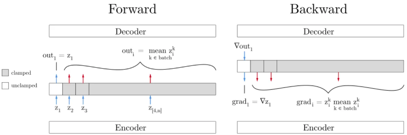
Encoder Decoder out = mean zk k ∈ batch i i grad = zk mean zk k ∈ batch i i i z[4,n] z3 z2 z1 out1 = z1 grad1 = ∇z1 ∇out1 Encoder Decoder clamped unclampedFigure 3-3: Training on a minibatch in which only 𝜑, the azimuth angle of the face, changes. During the forward step, the output from each component 𝑧𝑖 ̸= 𝑧1 of
the encoder is altered to be the same for each sample in the batch. This reflects the fact that the generating variables of the image (e.g. the identity of the face) which correspond to the desired values of these latents are unchanged throughout the batch. By holding these outputs constant throughout the batch, the single neuron 𝑧1 is forced
to explain all the variance within the batch, i.e. the full range of changes to the image caused by changing 𝜑. During the backward step 𝑧1 is the only neuron which receives
a gradient signal from the attempted reconstruction, and all 𝑧𝑖 ̸= 𝑧1 receive a signal
which nudges them to be closer to their respective averages over the batch. During the complete training process, after this batch, another batch is selected at random; it likewise contains variations of only one of 𝜑, 𝛼, 𝜑𝐿, 𝑖𝑛𝑡𝑟𝑖𝑛𝑠𝑖𝑐; all neurons which do
fixed but all other properties of the face change. That is, these batches consist of many different faces under the same viewing conditions and pose. These intrinsic properties of the model, which describe identity, shape, expression, etc., are represented by the remainder of the latent variables 𝑧[4,200]. These mini-batches varying intrinsic
properties are interspersed stochastically with those varying the extrinsic properties. We train this representation using SGVB, but we make some key adjustments to the outputs of the encoder and the gradients which train it. The procedure (Fig. 3-3) is as follows.
1. Select at random a latent variable 𝑧𝑡𝑟𝑎𝑖𝑛 which we wish to correspond to one of
{azimuth angle, elevation angle, azimuth of light source, intrinsic properties}. 2. Select at random a mini-batch in which that only that variable changes. 3. Show the network each example in the minibatch and capture its latent
repre-sentation for that example 𝑧𝑘.
4. Calculate the average of those representation vectors over the entire batch. 5. Before putting the encoder’s output into the decoder, replace the values 𝑧𝑖 ̸=
𝑧𝑡𝑟𝑎𝑖𝑛 with their averages over the entire batch. These outputs are “clamped”.
6. Calculate reconstruction error and backpropagate as per SGVB in the decoder. 7. Replace the gradients for the latents 𝑧𝑖 ̸= 𝑧𝑡𝑟𝑎𝑖𝑛 (the clamped neurons) with
their difference from the mean (see Sec. 3.3.2). The gradient at 𝑧𝑡𝑟𝑎𝑖𝑛 is passed
through unchanged.
8. Continue backpropagation through the encoder using the modified gradient. Since the intrinsic representation is much higher-dimensional than the extrinsic ones, it requires more training. Accordingly we select the type of batch to use in a ratio of about 1:1:1:10, azimuth : elevation : lighting : intrinsic; we arrived at this ratio after extensive testing, and it works well for both of our datasets.
This training procedure works to train both the encoder and decoder to represent certain properties of the data in a specific neuron. By clamping the output of all but one of the neurons, we force the decoder to recreate all the variation in that batch using only the changes in that one neuron’s value. By clamping the gradients, we
train the encoder to put all the information about the variations in the batch into one output neuron.
3.3.2
Invariance Targeting
By training with only one transformation at a time, we are encouraging certain neu-rons to contain specific information; this is equivariance. But we also wish to explicitly discourage them from having other information; that is, we want them to be invariant to other transformations. Since our mini-batches of training data consist of only one transformation per batch, then this goal corresponds to having all but one of the output neurons of the encoder give the same output for every image in the batch.
To encourage this property of the DC-IGN, we train all the neurons which corre-spond to the inactive transformations with an error gradient equal to their difference from the mean. It is simplest to think about this gradient as acting on the set of sub-vectors 𝑧𝑖𝑛𝑎𝑐𝑡𝑖𝑣𝑒 from the encoder for each input in the batch. Each of these 𝑧𝑖𝑛𝑎𝑐𝑡𝑖𝑣𝑒’s
will be pointing to a close-together but not identical point in a high-dimensional space; the invariance training signal will push them all closer together. We don’t care where they are; the network can represent the face shown in this batch however it likes. We only care that the network always represents it as still being the same face, no matter which way it’s facing. This regularizing force needs to be scaled to be much smaller than the true training signal, otherwise it can overwhelm the reconstruction goal. Empirically, a factor of 1/100 works well.
3.4
Experiments
We trained our model on about 12,000 batches of faces generated from a 3D face model obtained from Paysan et al. (2009), where each batch consists of 20 faces with random variations on face identity variables (shape/texture), pose, or lighting. We used the rmsprop (Tieleman and Hinton 2012) learning algorithm during training and set the meta learning rate equal to 0.0005, the momentum decay to 0.1 and weight decay to 0.01.
Figure 3-4: Manipulating light. Qualitative results showing the generalization capability of the learned DC-IGN decoder to re-render a single input image under different lighting conditions. We change the latent 𝑧𝑙𝑖𝑔ℎ𝑡 smoothly leaving all 199
Figure 3-5: Manipulating elevation. Results showing the ability of the DC-IGN decoder to change the elevation of the input image. We change the latent 𝑧𝑒𝑙𝑒𝑣𝑎𝑡𝑖𝑜𝑛
To ensure that these techniques work on other types of data, we also trained networks to perform reconstruction on images of widely varied 3D chairs from many perspectives derived from the Pascal Visual Object Classes dataset as extracted by Aubry et al. (Mottaghi et al. 2014, Aubry et al. (2014)). This task tests the ability of the DC-IGN to learn a rendering function for a dataset with high variation between the elements of the set; the chairs vary from office chairs to wicker to modern designs, and viewpoints span 360 degrees and two elevations. These networks were trained with the same methods and parameters as the ones above.
Figure 3-6: Manipulating azimuth (horizontal angle). Qualitative results show-ing the generalization capability of the learnt DC-IGN decoder to render original static image with different azimuth (pose) directions. The latent neuron 𝑧𝑎𝑧𝑖𝑚𝑢𝑡ℎ is
changed to random values but all other latents are clamped.
3.4.1
3D Face Dataset
The decoder network learns an approximate rendering engine as shown in Fig. 3-4. Given a static test image, the encoder network produces the latents 𝑍 depicting scene
variables such as light, pose, shape etc. Similar to an off-the-shelf rendering engine, we can independently control these to generate new images with the decoder. For example, as shown in Fig. 3-4, given the original test image, we can vary the lighting of an image by keeping all the other latents constant and varying 𝑧𝑙𝑖𝑔ℎ𝑡. It is perhaps
surprising that the fully-trained decoder network is able to function as a 3D rendering engine, and this capability is proof that the representation learned by the DC-IGN is disentangled.
We also quantitatively illustrate the network’s ability to represent pose and light on a smooth linear manifold as shown in Fig. 3-7, which directly demonstrates our training algorithm’s ability to disentangle complex transformations. In these plots, the inferred and ground-truth transformation values are plotted for a random subset of the test set. Interestingly, as shown in Fig. 3-7, the encoder network’s representation of azimuth has a discontinuity at 0∘ (facing straight forward).
3.4.2
Comparison with Entangled Representations
To explore how much of a difference the DC-IGN training procedure makes, we com-pare the novel-view reconstruction performance of networks with entangled represen-tations (baseline) versus disentangled represenrepresen-tations (DC-IGN). The baseline net-work is identical in every way to the DC-IGN, but was trained with SGVB without using our proposed training procedure. As in Fig. 3-6, we feed each network a single input image, then attempt to use the decoder to re-render this image at different azimuth angles. To do this, we first must figure out which latent of the entangled representation most closely corresponds to the azimuth. This we do rather simply. First, we encode all images in an azimuth-varied batch using the baseline’s encoder. Then we calculate the variance of each of the latents over this batch. The latent with the largest variance is then the one most closely associated with the azimuth of the face, and we will call it 𝑧𝑎𝑧𝑖𝑚𝑢𝑡ℎ. Once that is found, the latent 𝑧𝑎𝑧𝑖𝑚𝑢𝑡ℎ is varied for
both the models to render a novel view of the face given a single image of that face. Fig. 3-8 shows that explicit disentanglement is critical for novel-view reconstruction.
Figure 3-7: Generalization of decoder to render images in novel viewpoints and lighting conditions. We generated several datasets by varying light, azimuth and elevation, and tested the invariance properties of DC-IGN’s representation 𝑍. We show quantitative performance on three network configurations as described in Sec. 3.4.1. All DC-IGN encoder networks reasonably predicts transformations from static test images. Interestingly, as seen in the first plot, the encoder network seems to have learnt a switch node to deal uniquely with the mirror-symmetric sides of the face.
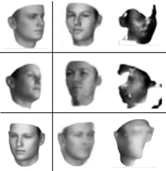
Figure 3-8: Entangled versus disentangled representations. First column: Original images. Second column: transformed image using DC-IGN. Third column: transformed image using normally-trained network.
3.4.3
Chair Dataset
We performed a similar set of experiments on the 3D chairs dataset described above. This dataset contains still images rendered from 3D CAD models of 1357 different chairs, each model skinned with the photographic texture of the real chair. Each of these models is rendered in 60 different poses; at each of two elevations, there are 30 images taken from 360 degrees around the model. We used approximately 1200 of these chairs in the training set and the remaining 150 in the test set; as such, the networks had never seen the chairs in the test set from any angle, so the tests explore the networks’ ability to generalize to arbitrary chairs. We resized the images to 150 × 150 pixels and made them grayscale to match our face dataset.
We trained these networks with the azimuth (flat rotation) of the chair as a dis-entangled variable represented by a single node 𝑧1; all other variation between images
is undifferentiated and represented by 𝑧[2,200]. The DC-IGN network succeeded in
achieving a mean-squared error (MSE) of reconstruction of 2.7722 × 10⁻⁴ on the test
Figure 3-9: Manipulating rotation: Each row was generated by encoding the input image (leftmost) with the encoder, then changing the value of a single latent and putting this modified encoding through the decoder. The network has never seen these chairs before at any orientation. Top: Some positive examples. Note that the DC-IGN is making a conjecture about any components of the chair it cannot see; in particular, it guesses that the chair in the top row has arms, because it can’t see that it doesn’t. Bottom: Examples in which the network extrapolates to new viewpoints less accurately.
In Fig. 3-9 we have included examples of the network’s ability to re-render previously-unseen chairs at different angles given a single image. For some chairs it is able to render fairly smooth transitions, showing the chair at many intermediate poses, while for others it seems to only capture a sort of “keyframes” representation, only having distinct outputs for a few angles. Interestingly, the task of rotating a chair seen only from one angle requires speculation about unseen components; the chair might have arms, or not; a curved seat or a flat one; etc.
4. Disentanglement in Computation
4.1
Introduction
While the learning of representation in fields such as vision and language have been extensively studied, representations in computation have only recently begun to be studied.
Instead of thinking about data, like images or text, representations of computation are about representing procedures, computation itself. Instead of representing an image, we might represent a transformation of that image, like rotating every object in it by 90°. Instead of representing the words in an English phrase, we might represent a program which translates it into French.
Every neural network can be thought of as a representation of a computation. The weights and nonlinearities in the networks combine to transform some input data to some output data; in action they are a function from an input domain to an output domain, and in storage they represent this function. The famous ImageNet network by Krizhevsky et al. (2012), for example, contains 60 million parameters which, along with their connectivity, define a function from an input domain of 256x256x3 image to a 1x1000 distribution over labels.
Applying our desiderata for representations, let us consider the quality of this 60-million-weight representation for a function which classifies images.
1. Disentangled: Just as any representation of data should be sparse over real transformations, the representation of the transformation itself should be sparse. The only clear factorization of the computation represented by a feedforward
neural network is the factorization into layers. Each layer of the network rep-resents a large matrix multiplication, and the function computed is the same for all inputs. This representation for computation is not at all sparse over its inputs, for the entire computation is performed no matter what the input is. 2. Interpretable: Neural networks are famously hard to interpret. Researchers
have developed whole classes of techniques for analyzing them, which use gra-dient ascent to visualize specific units of the network (Erhan et al. 2009), occlusions of the input to analyze significance (Zeiler and Fergus 2014), or in-verting their functions to visualize their information preservation (Mahendran and Vedaldi 2014). These techniques speak to the deeply uninterpretable nature of neural representations of computation.
3. Performant: Deep neural networks currently hold the accuracy records in almost every large-N dataset of image recognition, object localization, and phoneme recognition benchmark. In particular, this network set the record for ImageNet performance with an error rate more than 40% lower than any other entry.
4. Reusable: While substantial reuse of pretrained copies of this network has been made, such reuse is by no means simple. Typically the top half of the network is completely removed and another is trained (quite expensively) in its place; in other use cases the lower-level features generated by the first few layers of the network have been used directly as an embedding of the input space, with very mixed results. Compared with a more modular design, which might have separate components for localizing salient objects and determining various salient information about them (size, color, animacy, shape, context) this representation is quite hard to reuse.
5. Compact: This model contains 60 million parameters. It occupies hundreds of megabytes on disk when compressed. While those numbers sound large, it is not immediately clear if this is very large or very compact for a model which contains
all necessary information for determining the contents of arbitrary images. While this model performs extremely well, and might (in bad lighting, with the right Instagram filter) be considered compact, it is very far from ideal in disentan-glement, interpretability, and reusability. Just by disentangling the computation in this model, factorizing it into modules, its interpretability and reusability would be hugely improved.
If, for example, this network were disentangled by having a module which deter-mined whether a scene was indoors or outdoors and a separate classifier for each of those cases, we would gain several advantages:
• The indoor/outdoor classifier would be immediately comprehensible. • The indoor/outdoor classifier could be reused in other tasks.
• The location-specific object classifiers could be more easily interpreted (e.g. you would be very surprised if the indoor classifier predicted a train, or a gorilla). • The location-specific object classifiers would generate intermediate features which
were more diagnostic for other tasks in their given location.
To make an unfair comparison, let’s use our desiderata to consider the quality of a Python representation of the computation of the FizzBuzz problem:
def divisible_by_five(n): return n % 5 == 0 def divisible_by_three(n): return n % 3 == 0 def fizzbuzz(n): result = '' if divisible_by_three(n): result += 'fizz' if divisible_by_five(n):
result += 'buzz'
return result
def fizzbuzz_string(length):
result_list = map(fizzbuzz, range(1, length + 1))
return '\n'.join(result_list)
print(fizzbuzz_string(100))
1. Disentangled: This computation has been factorized into a number of distinct subcomponents, each of which is very small and can be used in multiple places. They do not depend on the state of the overall program, and have very low-dimensional and clearly-defined inputs and outputs. Simple operators such as += or % are composed into larger ones, and the contribution from each is very clear.
2. Interpretable: This representation can be easily read by anyone who knows how to program, and most of it could be understood even by people who don’t. 3. Performant: While this code will make no errors on the task, this is not a
meaningful question on a toy task.
4. Reusable: Individual components of this code represent functions which could be used elsewhere or for variants of this task. It would be trivial to use divisible_by_three anywhere else its functionality is needed, and the other functions can similarly be reused to generate FizzBuzz solutions of any length. 5. Compact: This representation occupies 370 bytes.
Our ideal representation of a computation would share the learnability and per-formance on hard problems of the deep network without giving up the goals of dis-entanglement and reuse quite so completely as the deep network does.
4.1.1
Catastrophic forgetting
One of the clearest demonstrations of the weakness of highly-entangled neural network representations of computation is catastrophic forgetting.
With the recent success of deep learning methods in many fields, efforts have been made to apply deep learning techniques to multitask learning problems. Deep learning is at the deepest level a method for hierarchically extracting good representations from complex data, with the higher levels of a network capturing increasingly abstract representations of the data. As such, deep learning seems naively to be a promising direction for multitask learning; abstract representations of the data should be useful for many related tasks, and the network should be able to simply not use any which are not helpful.
This theory has been borne out for simple, highly coupled tasks such as evaluating sentiment of reviews for different categories of products (Glorot, Bordes, and Bengio 2011). A more wide-ranging survey of deep learning methods for transfer and multi-task learning shows that some classes of models are able to improve their performance on the original, clean dataset after being shown perturbed or distorted versions of the same data (Bengio 2012).
However, even small changes in the task result in substantial changes to the op-timal features, especially at high levels of the network (Yosinski et al. 2014). This can lead to catastrophic forgetting, in which the network “unlearns” one task as it trains on another one. A recent set of experiments (Goodfellow et al. 2013) detail the tradeoff curve for performance on one task versus performance on the other task for both similar and dissimilar tasks. They show that for networks trained on two tasks, improvement on one task comes at a cost to performance on another.
This occurs because of the highly entangled nature of the computation carried out by these networks. When the network which is able to solve two different tasks is retrained on just one, it gradually mutates the calculations which are necessary in both of the tasks, until eventually it has repurposed them entirely for the use of the first task. What this system needs is a clear separation of concerns. If some functional
elements of the network were used only for one task, those elements would be safe to mutate at a high rate during training on that task. Similarly, those elements which were used across many tasks could change only very gradually, ensuring that even if one task is neglected for an extended period, the components it uses won’t have diverged too greatly from their original state.
In more specific terms, the problem is that each weight in the network receives gra-dients of a similar magnitude when training on either task. And with no parameters “reserved” for a specific task, that task is quickly forgotten.
4.2
Related Work
Until recently, work in this domain has largely centered around either a) learning programs in a fixed representation language, or b) jointly learning a program and its representation in e.g. a neural network, but with little attention focus on the representation itself. In particular, Liang et al. (Liang, Jordan, and Klein 2010) propose to learn programs via Bayesian inference with a grammar over a hierarchical structure. Zaremba et al. (2014) use an LSTM (Hochreiter and Schmidhuber 1997) to predict the output of simple programs written in Python; their effectiveness is remarkable, but the induced representation is so poor that the authors comment, “We do not know how heavily our model relies on memorization and how far the learned algorithm is from the actual, correct algorithm.”
A classic model that attempts to disentangle computation is the mixture of ex-perts (Jacobs, Jordan, and Barto 1991). However, as originally described this model was not especially successful at learning distinct functions for each expert; this led to a modification of the design which used sampling instead of weighting using the gating values (Jacobs et al. 1991). This modified design resulted in nicely decou-pled functions, but was much harder to train. Addressing this problem was a core inspiration for my work.
In the last year, work on learning structured representations of computation has become a popular topic. (Neelakantan, Le, and Sutskever 2015) augment a neural
network with a small set of hard-coded external operations which the network learns to use in multistep programs. (Reed and Freitas 2015) propose a very general model which similarly can use external programs, but with the addition of a call stack; however, this model requires strong supervision to train explicitly with the correct program trace, and as such is learning to recreate an existing program representa-tion. (Zaremba et al. 2015) use an external memory with pointers to learn routines for interacting with external data. (Graves, Wayne, and Danihelka 2014) perform complex operations on sequences such as sorting or repeatedly copying by using a differentiable content-based addressing mechanism to read and write to an external memory.
4.3
Controller-function networks
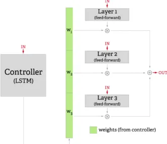
Figure 4-1: The controller and layers of the controller-function network (CFN).The controller provides weights on each layer as a function of the data. This shows three layers, but there can be many more.
The proposed model, the controller-function network (CFN) generates an output for a particular timestep via the following steps (shown in Fig. 4-1):
2. The controller decides which layers are most appropriate for processing this input
3. The controller outputs a weighting vector reflecting how much output it wants from each of the layers
4. The input tensor is fed into each layer (in parallel)
5. The outputs from each layer are multiplied by their respective weights from the controller
6. The weighted outputs from all the layers are summed together and output. This is the output of the whole network for this timestep.
Essentially the idea is that at each timestep, the controller examines the input that it gets, then produces a distribution over the activities of the various “functions” (single-layer NNs) which would best deal with this input. Since the controller is an LSTM, it can store information about the inputs it has received before, meaning that in a time series or language setting it can make weighting decisions contextually.
Each of the “function” layers is a single-layer network with a PReLU activation function (He et al. 2015). The input and output dimension of these functions is always the same, and corresponds to the desired output dimension of the network as a whole.
As this model is differentiable throughout, it can be trained with the standard backpropagation through time (BPTT) algorithm for stochastic gradient descent.
By setting weights over each of the layers in the network, the controller scales not only the output of each layer, but also the error gradient that it receives. This means that in a given timestep, the layers which have very low weights on their output will be nearly unchanged by the learning process. That is, functions which are not used are not forgotten.
In an ordinary feedforward neural network, the only way for the network to prevent learning in a particular node is for it to learn connection strengths very near zero for that node. This takes many training examples, and functionally removes that node from the computation graph.
on an input-by-input basis.
4.3.1
Relationship to mixture of experts
This architecture is closely related to the mixture of experts model proposed by Jacobs et al. (1991), in which several different task-specific “expert” networks each contribute in linear combination to the output of the overall network.
However, this model has two key differences from the mixture of experts:
1. The gating network is an LSTM. This means that the gating network (or controller, in my terminology) can easily learn fixed sequential procedures for certain types of input. This allow the model to be iterated for several steps, composing its operations into more complex ones. See Sec. 5.2.1 for a description of this usage.
2. The training results in decoupled functions. I employ a novel continuation method for training the CFN that allows for easy training, yet results in a final representation which uses only one “expert” at a time with no overlap.
4.3.2
Hard and soft decisions
Training neural models which make “hard” decisions can be quite challenging; in the general case, such models must be trained by REINFORCE-like gradient estima-tion methods (Williams 1992). Yet under many circumstances, such hard decisions are necessary for computational considerations; in fully-differentiable models such as the NTM (Graves, Wayne, and Danihelka 2014) or end-to-end memory networks (Sukhbaatar et al. 2015), the computational complexity of a single evaluation in-creases linearly with the size of the memory. These “soft” decisions involve considering every possible option.
In more complex computational tasks, such as those faced by (Reed and Freitas 2015), there may be a large number of steps before any result is produced by the model, and each step can require a discrete action (move the pointer either left or right; move the model either up or down). Such models naïvely have branching which
is exponential of the form 𝑂(𝑘𝑡), where 𝑘 is the number of options at each timestep,
and 𝑡 is the number of timesteps before producing an output. Using a REINFORCE algorithm to estimate the true gradient is possible, but slow and unreliable (Zaremba and Sutskever 2015). This branching factor is what led (Reed and Freitas 2015) to adopt their strongly-supervised training technique.
A straightforward (if inelegant) solution is to composite the outcome from all of these branches at the end of each timestep. For example, a pointer could be modeled as interpolating between two memory cells instead of having a discrete location. Then when the controller produces the distribution of actions “left 0.7, right 0.3”, the model can move the pointer left by 0.7 instead of sampling from 𝐵𝑒𝑟𝑛𝑜𝑢𝑙𝑙𝑖(0.7).
While such techniques, make the learning process tractable when available, they result in much more highly entangled representations (e.g. reading from a every loca-tion in a memory at once). Furthermore, they must always incur a complexity cost linear in the number of options, just as the memory models have cost linear in the number of options of memory locations to read from.
In especially challenging environments, this solution is not available. For example, in classic reinforcement learning tasks, the agent may only be in a situation once, and it cannot 70% fly to Germany or 20% accept a PhD position.
The CFN exists in the space of models for which this soft-decision solution is available. While in the ideal case we would like to select exactly one function to use at each timestep, this problem is quite difficult to optimize, for early in training the functions are not yet differentiated. By contrast, the soft-decision version which uses a weighted sum of the outputs of each function learns quite quickly. However, the solutions produced by this weighted sum training are highly entangled and always involve a linear combination of all the functions, with no clear differentiation.
From scratch, we can either train a system that works, or a system that has good representations. What we need is a way to go from a working solution to a good solution.
4.3.3
Continuation methods
Continuation methods are a widely-used technique for approaching difficult optimiza-tion problems.
In optimization by continuation, a transformation of the nonconvex func-tion to an easy-to-minimize funcfunc-tion is considered. The method then pro-gressively converts the easy problem back to the original function, while following the path of the minimizer. (Mobahi and Fisher III 2015)
As described in (Mobahi and Fisher III 2015), continuations include ideas as ubiq-uitous as curriculum learning or deterministic annealing, and that paper provides an extensive list of examples. In the quest for good solutions to hard-decision problems, continuation methods are a natural tool.
4.3.4
Training with noisy decisions
In order to construct a continuation between soft and hard decisions, the CFN com-bines two tools: weight sharpening and noise.
Weight sharpening is a technique used by (Graves, Wayne, and Danihelka 2014), which works by taking a distribution vector of weights 𝑤 ∈ [0, 1]𝑛, and a sharpening
parameter 𝛾 ≥ 1 and transforming 𝑤 as follows: 𝑤𝑖′ = 𝑤 𝛾 𝑖 ∑︀ 𝑗𝑤 𝛾 𝑗
By taking this [0, 1]𝑛 vector to an exponent, sharpening increases the relative
differences between the weights in 𝑤. Renormalizing makes 𝑤 a distribution once again, but now it has been stretched; large values are larger, i.e. the modes have higher probability. In the CFN, I take one further step: adding noise.
𝑤′𝑖 = (︀𝑤𝑖+𝒩 (0, 𝜎 2))︀𝛾 ∑︀ 𝑗𝑤 𝛾 𝑗
During the training of the CFN, sharpening is applied to the vector of weights produced by the controller, and the sharpening parameter 𝛾 is gradually increased on a schedule. By itself, this would not transform the outputs of the controller, as it can simply learn the inverse function to continue to produce the same output. However, the addition of noise before sharpening makes similar weights highly unstable. For example, if the network intended to produce a weighting of [0.5, 0.5], noise would interfere:
[0.49, 0.51]100
(0.49100+ 0.51100) = [0.018, 0.982]
At the end of training, this forces the CFN to either make a hard decision or face massive uncertainty in its output. By slowly increasing the sharpening parameter on a schedule, the controller can gradually learn to make harder and harder decisions. In practice this method works very well, resulting in perfectly binary decisions at the end of training and correct factorization of the primitives, each into its own function layer.
4.4
Experiments
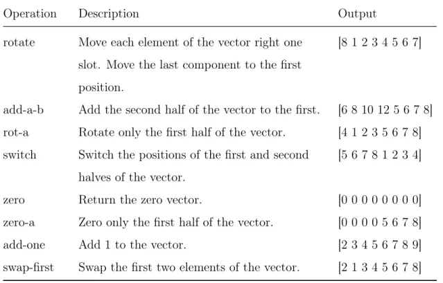
In order to carefully test the ability of various techniques to correctly factorize several presented problems, I constructed a simple dataset of vector functions, inputs, and outputs. These functions are detailed in Tbl. 4.1. In the following experiments, these functions are applied to random input vectors in [0, 1]10.
Since the inputs to all of these functions are indistinguishable, without any extra information it would be impossible for any system to achieve results better than averaging the output of all these functions. Therefore, along with the input vector, all systems receive a one-hot vector containing the index of the primitive to compute. Each system must learn to interpret this information in its own way. In the CFN, this metadata is passed only to the controller, which forces it to use different functions for different inputs.