HAL Id: hal-00461155
https://hal.archives-ouvertes.fr/hal-00461155
Submitted on 3 Mar 2010
HAL is a multi-disciplinary open access
archive for the deposit and dissemination of
sci-entific research documents, whether they are
pub-lished or not. The documents may come from
teaching and research institutions in France or
abroad, or from public or private research centers.
L’archive ouverte pluridisciplinaire HAL, est
destinée au dépôt et à la diffusion de documents
scientifiques de niveau recherche, publiés ou non,
émanant des établissements d’enseignement et de
recherche français ou étrangers, des laboratoires
publics ou privés.
strategies on production grids
Diane Lingrand, Johan Montagnat, Tristan Glatard
To cite this version:
Diane Lingrand, Johan Montagnat, Tristan Glatard. Estimating the execution context for refining
submission strategies on production grids. CCGrid, May 2008, Lyon, France. pp.753 – 758.
�hal-00461155�
submission strategies on production grids.
Diane Lingrand, Johan Montagnat, and Tristan Glatard
University of Nice - Sophia Antipolis / CNRS - FRANCE
[email protected], [email protected]
http://www.i3s.unice.fr/~ lingrand/
Abstract.
In this paper, we study grid job submission latencies. The
latency highly impacts performances on production grids, due to its high
values and variations as well as the presence of outliers. It is particularly
prejudicial for determining the status and expected duration of jobs.
In [1], a probabilistic model of the latency is presented that allows to
estimate the best timeout value considering a given distribution of jobs
latencies. This timeout value is then used in a job resubmission strategy.
The purpose of this paper is to evaluate to what extent updating this
model with relevant contextual parameters can help to refine the latency
estimation. Experiments on the EGEE grid show that the choice of the
resource broker or the computing site has a statistically significant
in-fluence on the jobs latency. We exploit this contextual information to
propose a reliable job submission strategy.
1
Motivations
Production grids are characterized by permanent but non-stationary load and a
large geographical extension. As a consequence, latency, measured as the time
between the submission time of a computation job and the beginning of its
execution, can be very high and experience large variations. As an example, on
the EGEE grid
1
(Enabling Grid for E-sciencE), the average latency is in the
order of 5 minutes with standard deviation also in the order of 5 minutes. This
variability is known to highly impact application performances and thus has to
be taken into account [2].
The main motivation for modeling the latency is to evaluate it precisely, hence
giving a reliable estimation of the expected job completion time. On an unreliable
grid infrastructure where a significant fraction of jobs is lost, this information
is valuable to set up an efficient resubmission strategy minimizing the impact
of faults. It can be exploited either at the workload management system level
or at the user level. Too long running jobs are canceled and resubmitted before
becoming too penalizing.
In [1], a probabilistic model of the latency is presented that allows to estimate
the best timeout value considering a given distribution of jobs latencies. This
timeout value is then used for job resubmission.
1
In a previous work [3], we have shown that some parameters from the
execu-tion context have an influence on the cumulative density funcexecu-tion of latency. In
this paper, we quantify their influence on the timeout values and the expected
execution time (including resubmissions). We aim at refining our model by
tak-ing into account most relevant contextual parameters in order to optimize our
job resubmission strategy.
2
Related works
Several initiatives aim at modeling grid infrastructure Workload Management
Systems (WMS). In [4], correlations between job execution properties (job size
or number of processors requested, job run time and memory used) are studied
on a multi-cluster supercomputer in order to build models of workloads, enabling
comparative study on system design and scheduling strategies. In [5], authors
make predictions of batch queue waiting time which improves the total execution
time.
Taking into account contextual information has been reported to help in
estimating single jobs and workflows execution time by rescheduling. Feitelson [6]
has observed correlations between run time and job size, number of cluster and
time of the day.
In [7], the influence of changes in transmission speed, in both executable code
and data size, and in failure likelihood are analysed for a better estimation of end
time of sub-workflows. This is used for re-scheduling jobs after fault or overrun.
Authors of [8] analyze job inter-arrival times, waiting times at the queues,
execution times and data exchanged sizes. They made experiments on the EGEE
grid on several VOs (Virtual Organizations) and studied the influence of the day
of the week and the time of the day. Their conclusion on these influences is that
there is an increase of the load at the end of the day and that it is difficult to
extract a precise model of the behavior with respect of the day or the time.
To refine the grid monitoring, [9] presents a model of the influence between
the grid components and their execution context (system and network levels),
experimented on Grid’5000.
In this paper, we aim at refining our grid model with more local and dynamic
parameters. Each job can be characterized by its execution context that depends
on the grid status and may evolve during the job life-cycle. The context of a job
depends both on parameters internal and external to the grid infrastructure. The
internal context corresponds to parameters such as the computer(s) involved in
the WMS of a specific job. It may not be completely known at the job submission
time. The external context is related to parameters such as the day of the week
that may be correlated to the grid workload.
3
Experimental platform
Our experiments are based on the EGEE production grid infrastructure. With
35000 CPUs dispatched world-wide in more than 240 computing centers, EGEE
represents an interesting case of study as it exhibits highly variable and quickly
evolving load patterns that depend on the concurrent activity of thousands of
potential users. The infrastructure is relatively homogeneous though as all
com-puter hosting middleware services are state of the art PC-compatible comcom-puters
running the same Operating System distribution (Scientific Linux v3) and hosted
in computing centers with very high speed connections to the Internet.
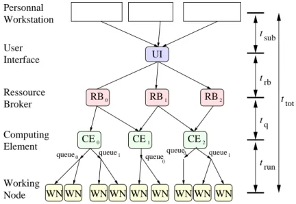
For the following discussion, the main components of the batch-oriented
EGEE grid infrastructure are introduced in figure 1.
t
tot
User
Interface
Ressource
Broker
Computing
Element
Working
Node
UI
RB
RB
CE
CE
CE
0
1
2
1
0
RB
2
t
t
t
t
sub
rb
q
run
Personnal
Workstation
WN
WN WN
WN
WN WN WN WN WN
queue
queue
queue
queue
0
1
0
1
queue
0
Fig. 1.
EGEE job life cycle
When a user want to submit a job from her workstation, she connects to an
EGEE client known as a User Interface (UI). A Resource Broker (RB) queues the
user requests and dispatches them to the different computing centers available.
The gateway to each computing center is one or more Computing Element (CE).
A CE hosts a batch manager that will distribute the workload over the center
Worker Nodes (WN), using different batch queues. Different queues are handling
jobs with different wall clock time. However the policies for deciding of the
number of queues and the maximal time assigned to each of them are
site-specific.
During its life-cycle, a job is characterized by its evolving status. Received by
the RB it is initially waiting, then queued at the CE and running on the WN. If
everything went right, the job is then completed. Otherwise, it is aborted,
timed-out
or in an error status depending on the type of failure. As shown in figure 1,
UIs can connect to different RBs, and RBs may be connected to overlapping sets
of CEs.
4
Modelisation of the grid
Models of the grid latency enable the optimization of job submission parameters
such as jobs granularity or the timeout value needed to make the WMS robust
against system faults and outliers. Properly modeling a large scale
infrastruc-ture is a challenging problem given its heterogeneity and its dynamic behavior.
In a previous work, we adopted a probabilistic approach [10] which proved to
improve application performances while decreasing the load applied on the grid
middleware by optimizing jobs granularities. Similar probabilistic models have
been proposed to estimate timeouts in other complex systems [11, 12].
In [1], we show how the distribution of the grid latency impacts the choice of
a timeout value for the jobs. We model the grid latency as a random variable R
with probability density function (pdf) f
R
and cumulative density function (cdf)
F
R
. The optimal timeout value can be obtained by minimizing the expectation of
the job execution time J which can be expressed as a function of R, the timeout
t
∞
and the proportion of outliers ρ:
E
J
(t
∞
) =
1
F
R
(t
∞
)
Z
t
∞
0
uf
R
(u)du +
t
∞
(1 − ρ)F
R
(t
∞
)
− t
∞
(1)
Taking into account contextual information has recently been reported to
help in estimating single jobs and workflows execution time by rescheduling [7].
We aim at refining our grid model with more local and dynamic parameters.
Each job can be characterized by its execution context that depends on the grid
status and may evolve during the job life-cycle. The context of a job depends
both on parameters internal and external to the grid infrastructure. The internal
context corresponds to parameters such as the computer(s) involved in the WMS
of a specific job. It may not be completely known at the job submission time.
The external context is related to parameters such as the day of the week and
may have an impact on the load imposed to the grid.
Our final goal is to improve job execution performance on grids. This
re-quires taking into account contextual information and its frequent update. In
this paper, we are studying some parameters among the broad range of
contex-tual information that could be envisaged and we discuss their relevance with
regard to grid infrastructures.
5
Experimental data and experiences plan
To study the grid latency, measures were collected by submitting a very large
number of probe jobs. These jobs, only consisting in the execution of an
al-most null duration /bin/hostname command, are only impacted by the grid
latency. In the reminder we make the hypothesis that the users job execution
time is known and that therefore only the grid latency varies significantly
be-tween different runs of the same computation task. To avoid variations of the
system load, a constant number of probes was executing inside the system at
any time of the data collection: a new probe was submitted each time another
one completed. For each probe job, we logged the job submission date, the UI
used, the UI load at submission time, the RB used, the CE used and the jobs
status duration (total duration t
tot
and partial durations t
sub
, t
rb
, t
q
and t
run
as illustrated in figure 1). The probe jobs were assigned a fixed 10000 seconds
timeout beyond which they were considered as outliers and canceled. This value
is far greater than the average latency observed. In average in our measurements
we observed a ρ = 3% ratio of outliers. We have observed that this ratio can
increase significantly sometimes due to system faults though.
Three measure Data Sets are considered in this paper:
DS1. 5800 probe jobs acquired during 10 days in September 2006 over 3 RBs and
92 CEs.
DS2. 7233 probe jobs acquired during 1 week in April 2007 over 1 RB and 3 CEs.
DS3
. 4173 probe jobs acquired during 1 week in May 2007 over 1 RB and 3 CEs.
These data sets were acquired randomly at very different times of the year to
avoid unexpected correlation with external events. They cover all days of the
week.
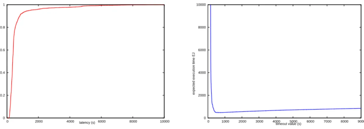
As an example, the cdf of the DS1 data set is plotted in figure 2. Its median
is 363 seconds, its expectation is 570 seconds and its standard deviation is 886
seconds, which quantifies the highly variable behavior of the EGEE grid. The first
part of this experimental distribution is close to a log-normal distribution and its
tail can be modeled by a Pareto distribution [1]. This heavy tailed distribution
shows that the EGEE grid exhibits non-negligible probabilities for long latencies.
0
0.2
0.4
F
0.6
0.8
1
0
2000
4000
latency (s) 6000
8000
10000
0
2000
4000
expected execution time EJ
6000
8000
10000
0
1000
2000
3000
4000
timeout value (s)
5000
6000
7000
8000
9000
Fig. 2.
Left: cumulative density function of the whole experimental data. Right:
expec-tation of the job execution time (in seconds), including resubmission, with respect to
the timeout value t
∞
(in seconds). The minimum of this curve gives the best timeout
In the remainder of the paper these measurements are exploited to quantify
the jobs latency and to evaluate the impact of various internal and external
con-text parameters. A concon-text-dependent optimal timeout value is thus computed.
It is the basis of an optimal resubmission strategy that aims at minimizing the
expected execution time of jobs submitted to the grid infrastructure. In
par-ticular, we consider in the following sections the impact of the target RB and
the target CE which are expected to have an influence on the latency due to
variable computing sites performance and variable load conditions. In addition,
the correlation between time of the day and latency is studied since external
parameters such as working and week-end days are expected to be correlated to
different system loads as well.
6
Influence of the Resource Broker (RB).
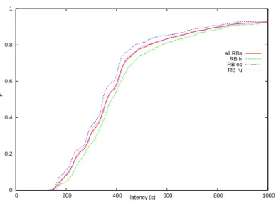
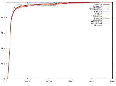
In this experiment, three different Resource Brokers were considered: a french one
(grid09.lal.in2p3.fr), a spanish one (egeerb.ifca.org.es) and a russian
one (lcg16.sinp.msu.ru). Their cdfs are shown in figure 3. The optimal timeout
values computed and the resulting expected execution time are reported below.
The table displays:
–
the optimal timeout value estimated and the difference between this value
and the global reference value obtained using all measurements without
dis-tinction;
–
the minimal expected execution time;
–
the expected execution time if the timeout is set to the global reference value
and the difference with the optimum.
all RBs
RB fr RB es RB ru
optimal t
∞
t
∞ref
= 556 s 729 s
546 s
506 s
∆t
∞
0%
31%
2%
9%
best E
J
479.125 s
483.7 s 445.2 s 476.2 s
E
J
(t
∞ref
)
479.125 s
488.8 s 445.9 s 477.9 s
∆E
J
0%
1%
0.2%
0.4%
The optimal timeout values obtained differ significantly and the most
dis-tinct is the one associated to the Spanish RB (variation of 31%). However, the
expected execution time varies by a much smaller amount (1% maximum). This
is related to the fact that in this case (relatively low outliers ratio and rather
ho-mogeneous infrastructure), slightly overestimating the timeout has little impact
on the execution time. It should be noted that an underestimation is impacting
the execution time much more though as can be seen in figure 4.
To simulate a more variable infrastructure, we applied the model
consider-ing a variable level of outliers between the different RBs (ρ = 20%, 3% and
0% respectively). These errors are realistic as error conditions regularly lead to
outliers ratios as high as 20%. The results are summarized in the following table:
0
0.2
0.4
F
0.6
0.8
1
0
200
400
latency (s)
600
800
1000
all RBs
RB fr
RB es
RB ru
Fig. 3.
Cumulative density function for the different Resource Brokers.
all RBs
RB fr RB es RB ru
ρ
7.7%
20%
3%
0%
optimal t
∞
t
∞ref
= 868 s 551 s
546 s
865 s
best E
J
452.3 s
639.8 s 445.2 s 451.7 s
E
J
(t
∞ref
)
452.3 s
691.7 s 456.2 s 451.7 s
∆E
J
0%
8%
2.5%
0%
In this case, the model consistently reports growing execution time disruptions
with the increase of the number of outliers. The resubmission strategy still rather
efficiently cope with the errors as the execution time variation does not exceed
8%. Taking into account the submission RB can help in adapting the optimal
timeout choice. The more variable the infrastructure, the more valuable the
optimization.
7
Influence of the Computing center
In a computing center, the batch submission system is usually configured with
several queues. The influence of the Computing Element (CE) and the associated
queues, later abbreviated as CE-queue, is considered in this section. The same
methodology than with RBs in section 6 could be envisaged but a significant
difference is that the number of CE-queues is much larger than the number of
RBs: in our experiment, we had 92 CEs and queues and 3 RBs. It might thus
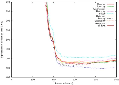
be relevant to group similar CE-queues to obtain fewer classes. As can be seen
in figure 4 many of the 92 CE-queues have similar cdfs while others are more
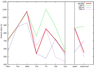
singular.
400
450
500
550
600
650
700
750
800
0
200
400
600
800
1000
expectation of execution time EJ (s)
timeout values (s)
Monday
Tuesday
Wednesday
Thursday
Friday
Saturday
Sunday
week only
week-end
all days
Fig. 4.
Expectation of job execution time with respect to the timeout value (t
∞
) for
the different CE and queues.
The idea we promote here is to group CEs and queues that have similar
properties into different classes.
7.1
Classification of the CE and queues
Different aggregations of CE-queues were tested based on their cdf using the
k-means classification algorithm with k = 2 to 10 classes. For each CE-queue
entity, the cdf has been computed. From this cdf the optimal timeout value is
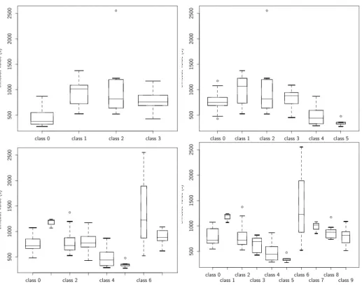
computed , by minimizing equation 1. Figures 5 and 6 show the repartition of
the timeout values in the classes. The depth of each box is proportional to the
number of CE-queues in the class.
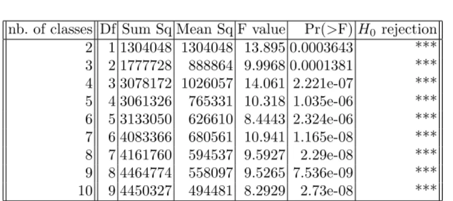
In order to measure if the classes are statistically discriminant, we have
tested the hypothesis H
0
(all set have equal mean and equal variance) using
ANOVA (ANalysis Of VAriance). The results are reported in the following table
nb. of classes Df Sum Sq Mean Sq F value
Pr(>F) H
0
rejection
2
1 1304048 1304048 13.895 0.0003643
***
3
2 1777728
888864 9.9968 0.0001381
***
4
3 3078172 1026057 14.061 2.221e-07
***
5
4 3061326
765331 10.318 1.035e-06
***
6
5 3133050
626610 8.4443 2.324e-06
***
7
6 4083366
680561 10.941 1.165e-08
***
8
7 4161760
594537 9.5927
2.29e-08
***
9
8 4464774
558097 9.5265 7.536e-09
***
10
9 4450327
494481 8.2929
2.73e-08
***
The result of the ANOVA test shows that these means differ significantly
with a probability lower than 0.1% in all cases. The best result is obtained for
9 classes but the gain is not so high. Note that the ANOVA test only show that
the hypothesis H
0
is rejected: this does not necessary imply that all classes differ
from each other.
In the case of 2 classes, these classes are statistically discriminant. But for all
other cases, further tests must be done in order to determine how many classes
are independent.
... ... ... ... ... . . . . . . . . . . . . . . . . . . . . . . . . . . . . . . . . . . . . . . . . . . . . . . . . . . . . . . . . . . . . . . . . . . . . . . . . . . . . . . . . . . . . . . . . . . . . . . . . . . . . . . . . . . . . . . . . . . . . . . . . . . . . . . . . . . . . . . . . . . . . . . . . . . . . . . . . . . . . . . . . . . . . . . . . . . . . . . . . . . . . . . . . . . . . . . . . . . . . . . . . . . . . . . . . . . . . . . . . . . . . . . . . ... . . . . . . . . . . . . . . . . . . . . . . . . . . . . . . . . . . . . . . . . . . . . . . . . . . . . . . . . . . . . . . . . . . . . . . . . ... . . ... . . ... . . ... ... . . . . . . . . . . . . . . . . . . . . . . . . . . . . . . . . . . . . . . . . . . . . . . . . . . . . . . . . . . . . . . . . . . . . . . . . . . . . . . . . . . . . . . . . . . . . . . ... ... ... . . . . . . . . . . . . . . . . . . . . . . . . . . . . . . . . . . . . . . . . . . . . . . . . . . . . . . . . . . . . . . . . . . . . . . . . . . . . . . . . . . . . . . . . . . . . . . . . . . . . . . . . . . . . . . . . . . . . . . . . . . . . . . . . . . . . . . . . . . . . . . . . . . . . . . . . . . . . . . . . . . . . . . . . . . . . . . . . . . . . . . . . . . . . . . . . . . . . . . ... . . . . . . . . . . . . . . . . . . . . . . . . . . . . . . . . . . . . . . . . ... ... ... ... . ... . . . . . . . . . . . . . . . . . . . . . . . . . . . . . . . . . . . . . . . . . . . . . . . . . . . . . . . . . . . . . . . . . . . . . . . . . . . . . . . . . . . . . . . . . . . . . . . . . . . . . . . . . . . . . . . . . . . . . . . . . . . . . . . . . . . . . . . . . . . . . . ... . . ... . . . . . . . . . . . . . . . . . . . . . .class 0
class 1
. . . . . . . . . . . . . . . . . . . . . . . . . . . . . . . . . . . . . . . . . . . . . . . . . . . . . . . . . . . . . . . . . . . . . . . . . . . . . . . . . . . . . . . . . . . . . . . . . . . . . . . . . . . . . . . . . . . . . . . . . . . . . . . . . . . . . . . . . . . . . . . . . . . . . . . . . . . . . . . . . . . . . . . . . . . . . . . . . . . . . . . . . . . . . . . . . . . . . . . . . . . . . . . . . . . . . . . . . . . . . . . . . . . . . . . . . . . . . . . . . . . . . . . . . . . . . . . . . . . . . . . . . . . . . . . . . . . . . . . . . . . . . . . . . . . . . . . . . . . . . . . . . . . . . . . . . . . . . . . . . . . . . . . . . . . . . . . . . . . . . . . . . . . . . . . . . . . . . . . . . . . . . . . . . . . . . . . . . . . . . . . . . . . . . . . . . . . . . . . . . . . . . . . . . . . . . . . . . . . . . . . . . . . . . . . . . . . . . . . . . . . . . . . . . . . . . . . . . . . . . . . . . . . . . . . . . . . . . . . . . . . . . . . . . . . . . . . . . . . . . . . . . . . . . . . . . . . . . . . . . .5
0
0
1
0
0
0
1
5
0
0
2
0
0
0
2
5
0
0
ti
m
eo
u
t
va
lu
e
(s
)
... . . . . . . . . . . . . . . . . . . . . . . . . . . . . . . . . . . . . . . . . . . . . . . . . . . . . . . . . . . . . . . . . . . . . . . . . . . . . . . . . . . . . . . . . . . . . . . . . . . . . . . . . . . . . . . . . . . . . . . . . . . . . . . . . . . . . . . . . . . . . . . . . . . . . . . . . . . . . . . . . . . . . . . . . . . . . . . . . . . . . . . . . . . . . . . . . . . . . . . . . . . . . . . . . . . . . . . . . . . . . . . . . . . . . . . . . . . . . . . . . . . . . . . . . . . . . . . . . . . . . . . . . . . . . . . . . . . . . . . . . . . . . . . . . . . . . . . . . . . . . . . . . . . . . . . . . . . . . . . . . . . . . . . . . . . . . . . . . . . . . . . . . . . . . . . . . . . . . . . . . . . . . . . . . . . . . . . . . . . . . . . . . . . . . . . . . . . . . . . . . . . . . . . . . . . . . . . . . . . . . . . . . . . . . . . . . . . . . . . . . . . . . . . . . . . . . . . . . . . . . . . . . . . . . . . . . . . . . . . . . . . . . . . . . . . . . . . . . . . . . . . . . . . . . . . . . . . . . . . . . . . . . . . . . . . . . . . . . . . . . . . . . . . . . . . . . . . . . . . . . . . . . . . . . . . . . . . ... ... ... . . . . . . . . . . . . . . . . . . . . . . . . . . . . . . . . . . . . . . . . . . . . . . . . . . . . . . . . . . . . . . . . . . . . . . . . . . . . . . . . . . . . . . . . . . . . . . . . . . . . . . . . . . . . . . . . . . . . . . . . . . . . . . . . . . . . . . . . . . . . . . . . . . . . . . . . . . . . . . . . . . . ... . . . . . . . . . . . . . . . . . . . . . . . . . . . . . . . . . . . . . . . . . . . . . . . . . . . . . . . . . . . . . . . . . . . . . . . . . . . ... . . ... . . ... . . ... . . ... . . ... . . ... . . . . . . . . . . . . . . . . . . . . . . . . . . . . . . . . . . . . . . . . . . . . . . . . . . . . . . . . . . . . . . . . . . . . . . . . . . . . . . . . . . . . . . . . ... ... . . . . . . . . . . . . . . . . . . . . . . . . . . . . . . . . . . . . . . . . . . . . . . . . . . . . . . . . . . . . . . . . . . . . . . . . . . . . . . . . . . . . . . . . . . . . . . . . . ... . . . . . . . . . . . . . . . . . . . . . . . . . . . . . . . . . . . . . . . . . . . . . . . . . . . . . . . . . . . . . . . . . . . . . . . . . . ... . ... . ... . ... . ... . ... . . ... . . . . . . . . . . . . . . . . . . . . . . . . . . . . . . . . . . . . . . . . . . . . . . . . . . . . . . . . . . . . . . . . . . . . . . . . . . . . . ... ... . . . . . . . . . . . . . . . . . . . . . . . . . . . . . . . . . . . . . . . . . . . . . . . . . . . . . . . . . . . . . . . . . . . . . . . . . . . . . . . . . . . . . . . . . . . . . . . . . . . . . . . . . . . . . . . . . . . . . . . . . . . . . . . . . . . . . . . . . . . . . . . . . . . . . . . . ... . . . . . . . . . . . . . . . . . . . . . . . . . . ... ... ... ... ... ... ... . . . . . . . . . . . . . . . . . . . . . . . . . . . . . . . . . . . . . . . . . . . . . . . . . . . . . . . . . . . . . . . . . . . . . . . . . . . . . . . . . . . . . . . . . . . . . . . . . . . . . . . . . . . . . . . . . . . . . . . . . . . . . . . . . . . . . . . . . . . . . ... . . ... . . . . . . . . . . . . . . . . . . . . . . . . . . . . . . . . .class 0
class 1
class 2
. . . . . . . . . . . . . . . . . . . . . . . . . . . . . . . . . . . . . . . . . . . . . . . . . . . . . . . . . . . . . . . . . . . . . . . . . . . . . . . . . . . . . . . . . . . . . . . . . . . . . . . . . . . . . . . . . . . . . . . . . . . . . . . . . . . . . . . . . . . . . . . . . . . . . . . . . . . . . . . . . . . . . . . . . . . . . . . . . . . . . . . . . . . . . . . . . . . . . . . . . . . . . . . . . . . . . . . . . . . . . . . . . . . . . . . . . . . . . . . . . . . . . . . . . . . . . . . . . . . . . . . . . . . . . . . . . . . . . . . . . . . . . . . . . . . . . . . . . . . . . . . . . . . . . . . . . . . . . . . . . . . . . . . . . . . . . . . . . . . . . . . . . . . . . . . . . . . . . . . . . . . . . . . . . . . . . . . . . . . . . . . . . . . . . . . . . . . . . . . . . . . . . . . . . . . . . . . . . . . . . . . . . . . . . . . . . . . . . . . . . . . . . . . . . . . . . . . . . . . . . . . . . . . . . . . . . . . . . . . . . . . . . . . . . . . . . . . . . . . . . . . . . . . . . . . . . . . . . . . . . .
5
0
0
1
0
0
0
1
5
0
0
2
0
0
0
2
5
0
0
ti
m
eo
u
t
va
lu
e
(s
)
. ... . . . . . . . . . . . . . . . . . . . . . . . . . . . . . . . . . . . . . . . . . . . . . . . . . . . . . . . . . . . . . . . . . . . . . . . . . . . . . . . . . . . . . . . . . . . . . . . . . . . . . . . . . . . . . . . . . . . . . . . . . . . . . . . . . . . . . . . . . . . . . . . . . . . . . . . . . . . . . . . . . . . . . . . . . . . . . . . . . . . . . . . . . . . . . . . . . . . . . . . . . . . . . . . . . . . . . . . . . . . . . . . . . . . . . . . . . . . . . . . . . . . . . . . . . . . . . . . . . . . . . . . . . . . . . . . . . . . . . . . . . . . . . . . . . . . . . . . . . . . . . . . . . . . . . . . . . . . . . . . . . . . . . . . . . . . . . . . . . . . . . . . . . . . . . . . . . . . . . . . . . . . . . . . . . . . . . . . . . . . . . . . . . . . . . . . . . . . . . . . . . . . . . . . . . . . . . . . . . . . . . . . . . . . . . . . . . . . . . . . . . . . . . . . . . . . . . . . . . . . . . . . . . . . . . . . . . . . . . . . . . . . . . . . . . . . . . . . . . . . . . . . . . . . . . . . . . . . . . . . . . . . . . . . . . . . . . . . . . . . . . . . . . . . . . . . . . . . . . . . . . . . . . . . . . . . . . .Fig. 5.
Timeout values repartition after k-mean classification into 2 classes (on the
left) and 3 classes (on the right) of CEs and queues.
7.2
Refining the ANOVA analysis
Let us look, for example, at the case of classification into 3 different classes
(classes 0, 1 and 2). Using ANOVA, if we test classes 1 and 2, we observe that
they do not differ significantly: F = 0.2334 (p < 0.6338). Building a new class,
class 1+2, from classes 1 and 2, we now test class 0 against class 1+2 and obtain
that they differ significantly: F = 19.651 (p < 3.003e − 05). We observe that
... ... . . . . . . . . . . . . . . . . . . . . . . . . . . . . . . . . . . . . . . . . . . . . . . . . . . . . . . . . . . . . . . . . . . . . . . . . . . . . . . . . . . . . . . . . . . . . . . . . . . . . . . . . ... . . . . . . . . . . . . . . . . . . . . . . . . . . . . . . . . . . . . . . . . . . . . . . . . . . . . . . . ... ... ... ... ... ... ... ... ... . . . . . . . . . . . . . . . . . . . . . . . . . . . . . . . . . . . . . . . . . . . . . . . . . . . . . . . . ... ... . . . . . . . . . . . . . . . . . . . . . . . . . . . . . . . . . . . . . . . . . . . . . . . . . . . . . . . . . . . . . . . . . . . . . . . . . . . . . . . . . . . . . . . . . . . . . . . . . . . . . . . . ... . . . . . . . . . . . . . . . . . . . . . . . . . . . . . . . . . . . . . . . . . . . . . . . . . . . . . . . . . . . . . . . . . . . . . . ... . . ... . . ... . . ... . . ... . . ... . . ... . . ... . . ... . . . . . . . . . . . . . . . . . . . . . . . . . . . . . . . . . . . . . . . . . . . . . . . . . . . . . . . . . . . . . . . . . . . . . . . . . . . . . . . . . . . . . . . . . . ... ... . . . . . . . . . . . . . . . . . . . . . . . . . . . . . . . . . . . . . . . . . . . . . . . . . . . . . . . . . . . . . . . . . . . . . . . . . . . . . . . . . . . . . . . . . . . . . . . . . . . . . . . . . . . . . . . . . . . . . . . . . . . . . . . . . . . . . . . . . . . . . . . . . . . . . . . . . . ... . . . . . . . . . . . . . . . . . . . . . . . . . . . . ... . . ... . . ... . . ... . . ... . . ... . . ... . . ... . . ... . . . . . . . . . . . . . . . . . . . . . . . . . . . . . . . . . . . . . . . . . . . . . . . . . . . . . . . . . . . . . . . . . . . . . . . . . . . . . . . . . . . . . . . . . . . . . . . . . . . . . . . . . . . . . . . . . . . . . . . . . . . . . . . . . . . . . . . . . . . . . . . . ... . . ... ... . . . . . . . . . . . . . . . . . . . . . . . . . . . . . . . . . . . . . . . . . . . . . . . . . . . . . . . . . . . . . . . . . . . . . . . . . . . . . . . . . . . . . . . . . . . . . . . . . . . . . . . . . . . . . . . . . . . . ... . . . . . . . . . . . . . . . . . . . . . . . . . . . . . . . . . . . . . . . . . . . . . . . . . . . . . . . . . . . . . . . . . . . . . . . . . ... ... ... ... ... ... ... ... . . ... . . . . . . . . . . . . . . . . . . . . . . . . . . . . . . . . . . . . . . . . . . . . . . . . . . . ... . . . . . . . . . . . . . . . . . . . . . . . . . . . . . . . . . . . . . . . . . . . .
class 0
class 1
class 2
class 3
. . . . . . . . . . . . . . . . . . . . . . . . . . . . . . . . . . . . . . . . . . . . . . . . . . . . . . . . . . . . . . . . . . . . . . . . . . . . . . . . . . . . . . . . . . . . . . . . . . . . . . . . . . . . . . . . . . . . . . . . . . . . . . . . . . . . . . . . . . . . . . . . . . . . . . . . . . . . . . . . . . . . . . . . . . . . . . . . . . . . . . . . . . . . . . . . . . . . . . . . . . . . . . . . . . . . . . . . . . . . . . . . . . . . . . . . . . . . . . . . . . . . . . . . . . . . . . . . . . . . . . . . . . . . . . . . . . . . . . . . . . . . . . . . . . . . . . . . . . . . . . . . . . . . . . . . . . . . . . . . . . . . . . . . . . . . . . . . . . . . . . . . . . . . . . . . . . . . . . . . . . . . . . . . . . . . . . . . . . . . . . . . . . . . . . . . . . . . . . . . . . . . . . . . . . . . . . . . . . . . . . . . . . . . . . . . . . . . . . . . . . . . . . . . . . . . . . . . . . . . . . . . . . . . . . . . . . . . . . . . . . . . . . . . . . . . . . . . . . . . . . . . . . . . . . . . . . . . . . . . . .
5
0
0
1
0
0
0
1
5
0
0
2
0
0
0
2
5
0
0
ti
m
eo
u
t
va
lu
e
(s
)
... . . . . . . . . . . . . . . . . . . . . . . . . . . . . . . . . . . . . . . . . . . . . . . . . . . . . . . . . . . . . . . . . . . . . . . . . . . . . . . . . . . . . . . . . . . . . . . . . . . . . . . . . . . . . . . . . . . . . . . . . . . . . . . . . . . . . . . . . . . . . . . . . . . . . . . . . . . . . . . . . . . . . . . . . . . . . . . . . . . . . . . . . . . . . . . . . . . . . . . . . . . . . . . . . . . . . . . . . . . . . . . . . . . . . . . . . . . . . . . . . . . . . . . . . . . . . . . . . . . . . . . . . . . . . . . . . . . . . . . . . . . . . . . . . . . . . . . . . . . . . . . . . . . . . . . . . . . . . . . . . . . . . . . . . . . . . . . . . . . . . . . . . . . . . . . . . . . . . . . . . . . . . . . . . . . . . . . . . . . . . . . . . . . . . . . . . . . . . . . . . . . . . . . . . . . . . . . . . . . . . . . . . . . . . . . . . . . . . . . . . . . . . . . . . . . . . . . . . . . . . . . . . . . . . . . . . . . . . . . . . . . . . . . . . . . . . . . . . . . . . . . . . . . . . . . . . . . . . . . . . . . . . . . . . . . . . . . . . . . . . . . . . . . . . . . . . . . . . . . . . . . . . . . . . . . . . . ... . . . . . . . . . . . . . . . . . . . . . . . . . . . . . . . . . . . . . . . ... . . . . . . . . . . . . . . . . . . . . . . . . . . . . . . . . . . . . . . . . . . . . . . . . . . . . . . . . . . . . . . . . . . ... . ... . ... . ... . ... . ... . ... . ... . ... . ... . ... . ... . ... . . . . . . . . . . . . . . . . . . . . . . . . . . . . . . . . . . . . . . . . . . . . . . . . ... . . . . . . . . . . ... . . . ... ... . . . . . . . . . . . . . . . . . . . . . . . . . . . . . . . . . . . . . . . . . . . . . . . . . . . . . . . . . . . . . . . . . . . . . . . . . . . . . . . . . . . . . . . . . . . . . . . . . . . . . . . . . . . . . . . . . . . . . . . . . . . . . . . . . . . . . . . . . . . . . . . . . . . . . . . . . . . ... . . . . . . . . . . . . . . . . . . . . . . . . . . . . . . . . . . . . . . . . . . . . . . . . . . . . . . . ... . ... . ... . ... . ... . ... . ... . ... . ... . ... . ... . ... . . . ... . . . . . . . . . . . . . . . . . . . . . . . . . . . . . . . . . . . . . . . . . . . . . . . . . . . . . . . . . . . . . . . . . . . . . . . . . . . . . . . . . . . . . . . . . . . . . . . . . . . . . . . . . . . . . . . . . . . . . . . ... . . . . . . . . . . . . . . . . . . . . . . . . . . . . . . . . . . . . . . . . . . . . . . . . . . . . . . . . . . . . . . . . . . . . . . . . . . . . . . . . . . . . . . . . . . . . . . . . . . . . . . . . . . . . . . . . . . . . . . . . . . . . . . . . . . . . . . . . . . . . . . . . . . . . . . . . . . ... . . . . . . . . . . . . . . . . . . . . . . . . . . . . ... . . ... . . ... . . ... . . ... . . ... . . ... . . ... . . ... . . ... . . ... . . ... . . ... . . . . . . . . . . . . . . . . . . . . . . . . . . . . . . . . . . . . . . . . . . . . . . . . . . . . . . . . . . . . . . . . . . . . . . . . . . . . . . . . . . . . . . . . . . . . . . . . . . . . . . . . . . . . . . . . . . . . . . . . . . . . . . . . . . . . . . . . . . . ... ... ... . . . . . . . . . . . . . . . . . . . . . . . . . . . . . . . . . . . . . . . . . . . . . . . . . . . . . . . . . . . . . . . . . . . . . . . . . . . . ... . . . . . . . . . . . . . . . . . . . . . . . . . . . . . . . . . . . . . . . . . . . . . . . . . . . . . . . . . . . . ... . ... . ... . ... . ... . ... . ... . ... . ... . ... . ... . ... ... . . . . . . . . . . . . . . . . . . . . . . . . . . . . . . . . . . . . . . . . . . . . . . . . . . . . . . ... ... . . . . . . . . . . . . . . . . . . . . . . . . . . . . . . . . . . . . . . . . . . . . . . . . . . . . . . . . . . . . . . . . . . . . . . . . . . . . . ... . . . . . . . . . . . . . . . . . . . . . . . . . . . . . . . . . . . . . . . . . . . . . . . . ... . ... . ... . ... . ... . ... . ... . ... . ... . ... . ... . ... . ... . . . . . . . . . . . . . . . . . . . . . . . . . . . . . . . . . . . . . . . . . . . . . . . . . . . . . . . . . . . . . . . . . ... . . . . . . . . . . . ... ... ... ... ... ... ... ... ... ... ... ... . ... . . . . . . . . . . . . . . . . . . . ... ... . . . . . . . . . . . . . . . . . . . . . . . . . . . . . . . . . . . . . . . . . . . . . . . . . . . . . . . . . . . . . . . . . .class 0
class 1
class 2
class 3
class 4
class 5
. . . . . . . . . . . . . . . . . . . . . . . . . . . . . . . . . . . . . . . . . . . . . . . . . . . . . . . . . . . . . . . . . . . . . . . . . . . . . . . . . . . . . . . . . . . . . . . . . . . . . . . . . . . . . . . . . . . . . . . . . . . . . . . . . . . . . . . . . . . . . . . . . . . . . . . . . . . . . . . . . . . . . . . . . . . . . . . . . . . . . . . . . . . . . . . . . . . . . . . . . . . . . . . . . . . . . . . . . . . . . . . . . . . . . . . . . . . . . . . . . . . . . . . . . . . . . . . . . . . . . . . . . . . . . . . . . . . . . . . . . . . . . . . . . . . . . . . . . . . . . . . . . . . . . . . . . . . . . . . . . . . . . . . . . . . . . . . . . . . . . . . . . . . . . . . . . . . . . . . . . . . . . . . . . . . . . . . . . . . . . . . . . . . . . . . . . . . . . . . . . . . . . . . . . . . . . . . . . . . . . . . . . . . . . . . . . . . . . . . . . . . . . . . . . . . . . . . . . . . . . . . . . . . . . . . . . . . . . . . . . . . . . . . . . . . . . . . . . . . . . . . . . . . . . . . . . . . . . . . . . .
5
0
0
1
0
0
0
1
5
0
0
2
0
0
0
2
5
0
0
ti
m
eo
u
t
va
lu
e
(s
)
. ... . . . . . . . . . . . . . . . . . . . . . . . . . . . . . . . . . . . . . . . . . . . . . . . . . . . . . . . . . . . . . . . . . . . . . . . . . . . . . . . . . . . . . . . . . . . . . . . . . . . . . . . . . . . . . . . . . . . . . . . . . . . . . . . . . . . . . . . . . . . . . . . . . . . . . . . . . . . . . . . . . . . . . . . . . . . . . . . . . . . . . . . . . . . . . . . . . . . . . . . . . . . . . . . . . . . . . . . . . . . . . . . . . . . . . . . . . . . . . . . . . . . . . . . . . . . . . . . . . . . . . . . . . . . . . . . . . . . . . . . . . . . . . . . . . . . . . . . . . . . . . . . . . . . . . . . . . . . . . . . . . . . . . . . . . . . . . . . . . . . . . . . . . . . . . . . . . . . . . . . . . . . . . . . . . . . . . . . . . . . . . . . . . . . . . . . . . . . . . . . . . . . . . . . . . . . . . . . . . . . . . . . . . . . . . . . . . . . . . . . . . . . . . . . . . . . . . . . . . . . . . . . . . . . . . . . . . . . . . . . . . . . . . . . . . . . . . . . . . . . . . . . . . . . . . . . . . . . . . . . . . . . . . . . . . . . . . . . . . . . . . . . . . . . . . . . . . . . . . . . . . . . . . . . . . . . . . . . . ... . . . . . . . . . . . . . . . . . . . . . . . . . . . . . . . . . . . . . . . . ... . . . . . . . . . . . . . . . . . . . . . . . . . . . . . . . . . . . . . . . . . . . . . . . . . . . . . . . . . . . . ... . ... . ... . ... . ... . ... . ... . ... . ... . ... . ... . ... . ... . ... . ... . ... . . ... . . . . . . . . . . . . . . . . . . . . . . . . . . . . . . . . . . . . . . . . . . . . . . . ... . . . . . . . . . . . . . . . . . . . . . . ... . . . . . . . . . . . . . . . ... ... ... ... ... ... ... ... ... ... ... ... ... ... ... ... ... . . . . . . . . . . . . . . . . . . . . . . ... ... . . . . . . . . . . . . . . . . . . . . . . . . . . . . . . . . . . . . . . . . . . . . . . . . . . . . . . . . . . . . . . . . . . . . . . . . . . . . ... . . . . . . . . . . . . . . . . . . . . . . . . . . . . . . . . . . . . . . . . . . . . . . . . . . . . . . . . . . . . . . ... ... ... ... ... ... ... ... ... ... ... ... ... ... ... ... ... . . . . . . . . . . . . . . . . . . . . . . . . . . . . . . . . . . . . . . . . . . . . . . . . . . . . . . . . . . . . . . . . . ... . . ... ... . . . . . . . . . . . . . . . . . . . . . . . . . . . . . . . . . . . . . . . . . . . . . . . . . . . . . . . . . . . . . . . . . . . . . . . . . . . . . . ... . . . . . . . . . . . . . . . . . . . . . . . . . . . . . . . . . . . . . . . . . . . . . . . . . . . . . . . . . . . . . . . . . . . . . . . . . ... . ... . ... . ... . ... . ... . ... . ... . ... . ... . ... . ... . ... . ... . ... . ... . . ... . . . . . . . . . . . . . . . . . . . . . . . . . . . . . . . . . . . . . . . . . . . . . . . . . . . . . ... ... . . . . . . . . . . . . . . . . . . . . . . . . . . . . . . . . . . . . . . . . . . . . . . . . . . . . . . . . . . . . . . . . . . . . . . . . . . . . . ... . . . . . . . . . . . . . . . . . . . . . . . . . . . . . . . . . . . . . . . . . . . . . . . . ... . ... . ... . ... . ... . ... . ... . ... . ... . ... . ... . ... . ... . ... . ... . ... . ... . . . . . . . . . . . . . . . . . . . . . . . . . . . . . . . . . . . . . . . . . . . . . . . . . . . . . . . . . . . . . . . . . ... . . . . . . . . . . . ... ... ... ... ... ... ... ... ... ... ... ... ... ... ... ... ... . . . . . . . . . . . . . . . . . . . ... ... . . . . . . . . . . . . . . . . . . . . . . . . . . . . . . . . . . . . . . . . . . . . . . . . . . . . . . . . . . . . . . . . . . . . . . . . . . . . . . . . . . . . . . . . . . . . . . . . . . . . . . . . . . . . . . . . . . . . . . . . . . . . . . . . . . . . . . . . . . . . . . . . . . . . . . . . . . . . . . . . . . . . . . . . . . . . . . . . . . . . . . . . . . . . . . . . . . . . . . . . . . . . . . . . . . . . . . . . . . . . . . . . . . . . . . . . . . . . . . . . . . ... . . . . . . . . . . . . . . . . . . . . . . . . . . . . . . . . . . . . . . . . . . . . . . . . . . . . . . . . . . . . . . . . . . . . . . . . . . . . . . . . . . . . . . . . . . . . . . . . . . . . . . . . . . . . . . . . . . . . . . . . . . . . . . . . . . . . . . . . ... . . ... . . ... . . ... . . ... . . ... . . ... . . ... . . ... . . ... . . ... . . ... . . ... . . ... . . ... . . ... ... . . . . . . . . . . . . . . . . . . . . . . . . . . . . . . . . . . . . . . . . . . . . . . . . . . . . . . . . . . . . . . . . . . . . . . . . . . . . . . . . . . . . . . . . . . . . . . . . . . . . . . . . . . . . . . . . . . . . . . . . . . . . . . . . . . . . . . . . . . . . . . . . . . . . . . . . . . . . . . . . . . . . . . . . . . . . . . . . . . . . . . . . . . . . . . . . . . . . . . . . . . . . . . . . . . . . . . . . . . . . . . . . . . . . . . . . . . . . . . . . ... ... . . . . . . . . . . . . . . . . . . . . . . . . . . . . . . . . . . . . . . . . . . . . . . . . . . . . . . . . . . . . . . . . . . . . . . . . . . . . . . ... . . . . . . . . . . . . . . . . . . . . . . . . . . . . . . . . . . . . . . . . ... ... ... ... ... ... ... ... ... ... ... ... ... ... ... ... . . ... . . . . . . . . . . . . . . . . . . . . . . . . . . . . . . . . . . . . . . . . . . . . . . . . . . . ... . . . . . . . . . . . . . . . . . . . . . . . . . . . . . . . . . . . . . . . . . . . . . . . . . . . . . . . . . . . . . . . . . . . . . . . . . . . . . . . . . . . . . . . .class 0
class 2
class 4
class 6
. . . . . . . . . . . . . . . . . . . . . . . . . . . . . . . . . . . . . . . . . . . . . . . . . . . . . . . . . . . . . . . . . . . . . . . . . . . . . . . . . . . . . . . . . . . . . . . . . . . . . . . . . . . . . . . . . . . . . . . . . . . . . . . . . . . . . . . . . . . . . . . . . . . . . . . . . . . . . . . . . . . . . . . . . . . . . . . . . . . . . . . . . . . . . . . . . . . . . . . . . . . . . . . . . . . . . . . . . . . . . . . . . . . . . . . . . . . . . . . . . . . . . . . . . . . . . . . . . . . . . . . . . . . . . . . . . . . . . . . . . . . . . . . . . . . . . . . . . . . . . . . . . . . . . . . . . . . . . . . . . . . . . . . . . . . . . . . . . . . . . . . . . . . . . . . . . . . . . . . . . . . . . . . . . . . . . . . . . . . . . . . . . . . . . . . . . . . . . . . . . . . . . . . . . . . . . . . . . . . . . . . . . . . . . . . . . . . . . . . . . . . . . . . . . . . . . . . . . . . . . . . . . . . . . . . . . . . . . . . . . . . . . . . . . . . . . . . . . . . . . . . . . . . . . . . . . . . . . . . . . .
5
0
0
1
0
0
0
1
5
0
0
2
0
0
0
2
5
0
0
ti
m
eo
u
t
va
lu
e
(s
)
... . . . . . . . . . . . . . . . . . . . . . . . . . . . . . . . . . . . . . . . . . . . . . . . . . . . . . . . . . . . . . . . . . . . . . . . . . . . . . . . . . . . . . . . . . . . . . . . . . . . . . . . . . . . . . . . . . . . . . . . . . . . . . . . . . . . . . . . . . . . . . . . . . . . . . . . . . . . . . . . . . . . . . . . . . . . . . . . . . . . . . . . . . . . . . . . . . . . . . . . . . . . . . . . . . . . . . . . . . . . . . . . . . . . . . . . . . . . . . . . . . . . . . . . . . . . . . . . . . . . . . . . . . . . . . . . . . . . . . . . . . . . . . . . . . . . . . . . . . . . . . . . . . . . . . . . . . . . . . . . . . . . . . . . . . . . . . . . . . . . . . . . . . . . . . . . . . . . . . . . . . . . . . . . . . . . . . . . . . . . . . . . . . . . . . . . . . . . . . . . . . . . . . . . . . . . . . . . . . . . . . . . . . . . . . . . . . . . . . . . . . . . . . . . . . . . . . . . . . . . . . . . . . . . . . . . . . . . . . . . . . . . . . . . . . . . . . . . . . . . . . . . . . . . . . . . . . . . . . . . . . . . . . . . . . . . . . . . . . . . . . . . . . . . . . . . . . . . . . . . . . . . . . . . . . . . . . ... . . . . . . . . . . . . . . . . . . . . . . . . . . . . . . . . . . . . . . . . . . . . . . . . . . . . . . . . . . . . . . . . . . . . . . . . . . . . . ... . . . . . . . . . . . . . . . . . . . . . . . . . . . . . . . . . . . . . . . . . . ... . ... . ... . ... . ... . ... . ... . ... . ... . ... . ... . ... . ... . ... . ... . ... . ... . ... . ... . ... . ... . . . . . . . . . . . . . . . . . . . . . . . . . . . . . . . . . . . . . . . . . . . . . . . . . . . . . . . . . . . . . . . . . . . . ... . . . . . . . . . . . . . . . . . . . . ... . . . . . . . . . . . . . . . ... ... ... ... ... ... ... ... ... ... ... ... ... ... ... ... ... ... ... ... ... . . . . . . . . . . . . . . . . . . . . . ... . . . . . . . . . . . . . . . . . . . . . . . . . . . . . . . . . . . . . . . . . . . . . . . . . . . . . . . . . . . . . . . . . . . . . . . . . . . . . ... . . . . . . . . . . . . . . . . . . . . . . . . . . . . . . . . . . . . . . . . . . . . . . . . . . . . . . . . . . . . . . . ... . ... . ... . ... . ... . ... . ... . ... . ... . ... . ... . ... . ... . ... . ... . ... . ... . ... . ... . ... . ... . . . . . . . . . . . . . . . . . . . . . . . . . . . . . . . . . . . . . . . . . . . . . . . . . . . . . . . . . . . . . . . . . . ... . ... . . . . . . . . . . . . . . . . . . . . . . . . . . . . . . . . . . . . . . . . . . . . . . . . . . . . . . . . . . . . . . . . . . . . . . . . . . . . . ... . . . . . . . . . . . . . . . . . . . . . . ... ... ... ... ... ... ... ... ... ... ... ... ... ... ... ... ... ... ... ... . ... . . . . . . . . . . . . . . . . . . . . . . . . . . . . . . . . . . . . . . . . . . . . . . . . . . . . . . . . . . . . . . . . . . . . ... . . . . . . . . . . . . . . . . . . . . . . . . . . . . . . . . . . . . . . . . . . . . . . . . . . . . . . . . . . . . . . . . . . . . . . . . . . . . ... . . . . . . . . . . . . . . . . . . . . . . . . . . . . . . . . . . . . . . . . . . . . . . . ... ... ... ... ... ... ... ... ... ... ... ... ... ... ... ... ... ... ... ... ... . . . . . . . . . . . . . . . . . . . . . . . . . . . . . . . . . . . . . . . . . . . . . . . . . . . . . . . . . . . . . . . . ... . . . . . . . . . . . ... ... ... ... ... ... ... ... ... ... ... ... ... ... ... ... ... ... ... ... . . ... . . . . . . . . . . . . . . . . . . . . . . ... ... . . . . . . . . . . . . . . . . . . . . . . . . . . . . . . . . . . . . . . . . . . . . . . . . . . . . . . . . . . . . . . . . . . . . . . . . . . . . . . . . . . . . . . . . . . . . . . . . . . . . . . . . . . . . . . . . . . . . . . . . . . . . . . . . . . . . . . . . . . . . . . . . . . . . . . . . . . . . . . . . . . . . . . . . . . . . . . . . . . . . . . . . . . . . . . . . . . . . . . . . . . . . . . . . . . . . . . . . . . . . . . . . . . . . . . . . . . . . . . . ... . . . . . . . . . . . . . . . . . . . . . . . . . . . . . . . . . . . . . . . . . . . . . . . . . . . . . . . . . . . . . . . . . . . . . . . . . . . . . . . . . . . . . . . . . . . . . . . . . . . . . . . . . . . . . . . . . . . . . . . . . . . . . . . . . . . . . . . ... . ... . ... . ... . ... . ... . ... . ... . ... . ... . ... . ... . ... . ... . ... . ... . ... . ... . ... . ... ... . . . . . . . . . . . . . . . . . . . . . . . . . . . . . . . . . . . . . . . . . . . . . . . . . . . . . . . . . . . . . . . . . . . . . . . . . . . . . . . . . . . . . . . . . . . . . . . . . . . . . . . . . . . . . . . . . . . . . . . . . . . . . . . . . . . . . . . . . . . . . . . . . . . . . . . . . . . . . . . . . . . . . . . . . . . . . . . . . . . . . . . . . . . . . . . . . . . . . . . . . . . . . . . . . . . . . . . . . . . . . . . . . . . . . . . . . . . . . . ... . . . . . . . . . . . . . . . . . . . . . . . . . . . ... . . . . . . . . . . . . . . . . . . . ... ... ... ... ... ... ... ... ... ... ... ... ... ... ... ... ... ... ... ... ... . . . . . . . . . . . . . . . . . . . . . . . . . . . . . ... ... . . . . . . . . . . . . . . . . . . . . . . . . . . . . . . . . . . . . . . ... . . . . . . . . . . . . . . . . . . . . . . ... . . ... . . ... . . ... . . ... . . ... . . ... . . ... . . ... . . ... . . ... . . ... . . ... . . ... . . ... . . ... . . ... . . ... . . ... . . ... . ... . . . . . . . . . . . . . . . . . . . . . . . . . . . . . . . . . . . . . . . . . . . . . . . ... . . ... . . . . . . . . . . . . . . . . . . . . . . . . . . . . . . . . . . . . . . . . . . . . . . . . . . . . . . . . . . . . . . . . . . . . . . . . . . . . . . ... . . . . . . . . . . . . . . . . . . . . . . . . . . . . . . . . . . . . . . . . . . . . . . . . . . . . . . ... . . ... . . ... . . ... . . ... . . ... . . ... . . ... . . ... . . ... . . ... . . ... . . ... . . ... . . ... . . ... . . ... . . ... . . ... . . ... . . ... . . . . . . . . . . . . . . . . . . . . . . . . . . . . . . . . . . . . . . . . . . . . . . . . . . . . . . . ... . . . . . . . . . . . . . . . . . . . . . . . . . . . . . . . . . . . . . . . . . . . . . . . . . . . . . . . . . . . . . . . . . . . . . . . . . . . . . . . . . . . . . . . . . . . . . . . . . . . . . . . . . . . . . .class 0
class 1
class 2
class 3
class 4
class 5
class 6
class 7
class 8
class 9
. . . . . . . . . . . . . . . . . . . . . . . . . . . . . . . . . . . . . . . . . . . . . . . . . . . . . . . . . . . . . . . . . . . . . . . . . . . . . . . . . . . . . . . . . . . . . . . . . . . . . . . . . . . . . . . . . . . . . . . . . . . . . . . . . . . . . . . . . . . . . . . . . . . . . . . . . . . . . . . . . . . . . . . . . . . . . . . . . . . . . . . . . . . . . . . . . . . . . . . . . . . . . . . . . . . . . . . . . . . . . . . . . . . . . . . . . . . . . . . . . . . . . . . . . . . . . . . . . . . . . . . . . . . . . . . . . . . . . . . . . . . . . . . . . . . . . . . . . . . . . . . . . . . . . . . . . . . . . . . . . . . . . . . . . . . . . . . . . . . . . . . . . . . . . . . . . . . . . . . . . . . . . . . . . . . . . . . . . . . . . . . . . . . . . . . . . . . . . . . . . . . . . . . . . . . . . . . . . . . . . . . . . . . . . . . . . . . . . . . . . . . . . . . . . . . . . . . . . . . . . . . . . . . . . . . . . . . . . . . . . . . . . . . . . . . . . . . . . . . . . . . . . . . . . . . . . . . . . . . . . .
5
0
0
1
0
0
0
1
5
0
0
2
0
0
0
2
5
0
0
ti
m
eo
u
t
va
lu
e
(s
)
. ... . . . . . . . . . . . . . . . . . . . . . . . . . . . . . . . . . . . . . . . . . . . . . . . . . . . . . . . . . . . . . . . . . . . . . . . . . . . . . . . . . . . . . . . . . . . . . . . . . . . . . . . . . . . . . . . . . . . . . . . . . . . . . . . . . . . . . . . . . . . . . . . . . . . . . . . . . . . . . . . . . . . . . . . . . . . . . . . . . . . . . . . . . . . . . . . . . . . . . . . . . . . . . . . . . . . . . . . . . . . . . . . . . . . . . . . . . . . . . . . . . . . . . . . . . . . . . . . . . . . . . . . . . . . . . . . . . . . . . . . . . . . . . . . . . . . . . . . . . . . . . . . . . . . . . . . . . . . . . . . . . . . . . . . . . . . . . . . . . . . . . . . . . . . . . . . . . . . . . . . . . . . . . . . . . . . . . . . . . . . . . . . . . . . . . . . . . . . . . . . . . . . . . . . . . . . . . . . . . . . . . . . . . . . . . . . . . . . . . . . . . . . . . . . . . . . . . . . . . . . . . . . . . . . . . . . . . . . . . . . . . . . . . . . . . . . . . . . . . . . . . . . . . . . . . . . . . . . . . . . . . . . . . . . . . . . . . . . . . . . . . . . . . . . . . . . . . . . . . . . . . . . . . . . . . . . . . .Fig. 6.
Timeout values repartition after k-mean classification into 4, 6, 8 and 10 classes
of CE-queues.
... ... ... ... ... . . . . . . . . . . . . . . . . . . . . . . . . . . . . . . . . . . . . . . . . . . . . . . . . . . . . . . . . . . . . . . . . . . . . . . . . . . . . . . . . . . . . . . . . . . . . . . . . . . . . . . . . . . . . . . . . . . . . . . . . . . . . . . . . . . . . . . . . . . . . . . . . . . . . . . . . . . . . . . . . . . . . . . . . . . . . . . . . . . . . . . . . . . . . . . . . . . . . . . . . . . . . . . ... . . . . . . . . . . . . . . . . . . . . . . . . . . . . . . . . . . . . . . . . . . . . . . . . . . . . . . . . . . . . . . . . . . . . . . . . . ... ... ... ... ... . . . . . . . . . . . . . . . . . . . . . . . . . . . . . . . . . . . . . . . . . . . . . . . . . . . . . . . . . . . . . . . . . . . . . . . . . . . . . . . . . . . . . . ... ... ... . . . . . . . . . . . . . . . . . . . . . . . . . . . . . . . . . . . . . . . . . . . . . . . . . . . . . . . . . . . . . . . . . . . . . . . . . . . . . . . . . . . . . . . . . . . . . . . . . . . . . . . . . . . . . . . . . . . . . . . . . . . . . . . . . . . . . . . . . . . . . . . . . . . . . . . . . . . . . . . . . . . . . . . . . . . . . . . . . . . . . . . . . . . . . . . . . . . . . . . . . . . . . . . . . . . . ... . . . . . . . . . . . . . . . . . . . . . . . . . . . . . . . . . . . . . . . . . . . . . . . . . . . . . . . . . . ... . . . ... . . . ... . . . ... . . ... . . . . . . . . . . . . . . . . . . . . . . . . . . . . . . . . . . . . . . . . . . . . . . . . . . . . . . . . . . . . . . . . . . . . . . . . . . . . . . . . . . . . . . . . . . . . . . . . . . . . . . . . . . . . . . . . . . . . . . . . . ... . . ... . . . . . . . . . . . . . . . . . . . . . .class 0
class 1 2
. . . . . . . . . . . . . . . . . . . . . . . . . . . . . . . . . . . . . . . . . . . . . . . . . . . . . . . . . . . . . . . . . . . . . . . . . . . . . . . . . . . . . . . . . . . . . . . . . . . . . . . . . . . . . . . . . . . . . . . . . . . . . . . . . . . . . . . . . . . . . . . . . . . . . . . . . . . . . . . . . . . . . . . . . . . . . . . . . . . . . . . . . . . . . . . . . . . . . . . . . . . . . . . . . . . . . . . . . . . . . . . . . . . . . . . . . . . . . . . . . . . . . . . . . . . . . . . . . . . . . . . . . . . . . . . . . . . . . . . . . . . . . . . . . . . . . . . . . . . . . . . . . . . . . . . . . . . . . . . . . . . . . . . . . . . . . . . . . . . . . . . . . . . . . . . . . . . . . . . . . . . . . . . . . . . . . . . . . . . . . . . . . . . . . . . . . . . . . . . . . . . . . . . . . . . . . . . . . . . . . . . . . . . . . . . . . . . . . . . . . . . . . . . . . . . . . . . . . . . . . . . . . . . . . . . . . . . . . . . . . . . . . . . . . . . . . . . . . . . . . . . . . . . . . . . . . . . . . . . . . .5
0
0
1
0
0
0
1
5
0
0
2
0
0
0
2
5
0
0
classes
ti
m
eo
u
t
va
lu
e
(s
)
... . . . . . . . . . . . . . . . . . . . . . . . . . . . . . . . . . . . . . . . . . . . . . . . . . . . . . . . . . . . . . . . . . . . . . . . . . . . . . . . . . . . . . . . . . . . . . . . . . . . . . . . . . . . . . . . . . . . . . . . . . . . . . . . . . . . . . . . . . . . . . . . . . . . . . . . . . . . . . . . . . . . . . . . . . . . . . . . . . . . . . . . . . . . . . . . . . . . . . . . . . . . . . . . . . . . . . . . . . . . . . . . . . . . . . . . . . . . . . . . . . . . . . . . . . . . . . . . . . . . . . . . . . . . . . . . . . . . . . . . . . . . . . . . . . . . . . . . . . . . . . . . . . . . . . . . . . . . . . . . . . . . . . . . . . . . . . . . . . . . . . . . . . . . . . . . . . . . . . . . . . . . . . . . . . . . . . . . . . . . . . . . . . . . . . . . . . . . . . . . . . . . . . . . . . . . . . . . . . . . . . . . . . . . . . . . . . . . . . . . . . . . . . . . . . . . . . . . . . . . . . . . . . . . . . . . . . . . . . . . . . . . . . . . . . . . . . . . . . . . . . . . . . . . . . . . . . . . . . . . . . . . . . . . . . . . . . . . . . . . . . . . . . . . . . . . . . . . . . . . . . . . . . . . . . . . . . .0
0.2
0.4
F
0.6
0.8
1
0
2000
4000
latency (s) 6000
8000
10000
"class 0"
"classes 1 and 2"
"whole class 0"
"whole classes 1 and 2"
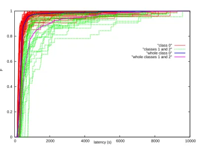
Fig. 8.
Cumulative density functions of latency with respect to time (in seconds). This
figure is obtained from the k-means classification into 3 classes. We grouped the last 2
classes into a single one so that we have 2 classes: the initial class 0 (in red) and new
class 3 (in green) resulting of the merging of classes 1 and 2. Each curve corresponds
to the cdf of one CE-queue. The curves in blue and magenta correspond to the global
cdf for class 0 (in blue) and class 3 (in magenta).
grouping two classes after the classification k = 3 gives a similar although slightly
better result than the classification k = 2.
The optimal timeout for the 2 populations (classes 0 and 3) are t
∞
0
= 779s
and t
∞
3
= 881s respectively (see figure 8).
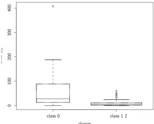
Figure 9 shows the errors computed between the best E
J
and E
J
(t
∞
), where
t
∞
if computed from the whole class.
. . ... ... ... . . . . . . . . . . . . . . . . . . . . . . . . . . . . . . . . . . . . . . . . . . . . . . . . . . . . . . . . . . . . . . . . . . . . . . . . . . . . . . . . . . . . . . . . . . . . . . . . . . . . . . . . . . . . . . . . . . . . . . . . . . . . . . . . . . . . . . . . . . . . . . . . . . . . . . . . . . . . . . . . . . . . . . . . . . . . . . . . . . . . . . . . . . . . . . ... . . . . . . . . . . . . . . . . . . . . . . . . . . . . . . . . . . . . . . . . . . . . . . . . . . . . . . . . . . . . . . . . . . . . . . . . . . . . . . . . . . . . . . . . . ... . . ... . . ... . . ... . . ... . . . . . . . . . . . . . . . . . . . . . . . . . . . . . . . . . . . . . . . . . . . . . . . . . . . . . . . . . . . . . . . . . . . . . . . . . . . . . . . . . . . . . . . . . . . . . . . . . . . . . . . . . . . . . ... . ... ... ... ... ... . . . . . . . . . . . . . . ... . . . . . . . . . . . . . . ... ... ... ... . ... . . . . . . . . . . . . . . . . . . . . . . . ... . . . . . . . . . ... . . . . . . . . . ... . . . . . . . . . ... . . . . . . ... . . . . . . . . . ... . ... . . . . . . . . . . . . . . . . . . . . . .