Dynamique agéostrophique dans l'océan intérieur

HAL Id: tel-02998433

https://tel.archives-ouvertes.fr/tel-02998433

Submitted on 10 Nov 2020

HAL is a multi-disciplinary open access

archive for the deposit and dissemination of

sci-entific research documents, whether they are

pub-lished or not. The documents may come from

teaching and research institutions in France or

abroad, or from public or private research centers.

L’archive ouverte pluridisciplinaire HAL, est

destinée au dépôt et à la diffusion de documents

scientifiques de niveau recherche, publiés ou non,

émanant des établissements d’enseignement et de

recherche français ou étrangers, des laboratoires

publics ou privés.

Dynamique agéostrophique dans l’océan intérieur

Lia Siegelman

To cite this version:

Lia Siegelman. Dynamique agéostrophique dans l’océan intérieur. Sciences de la Terre. Université de

Bretagne occidentale - Brest, 2019. Français. �NNT : 2019BRES0094�. �tel-02998433�

T

HESE DE DOCTORAT DE

L

'UNIVERSITE

DE

BRETAGNE

OCCIDENTALE

C

OMUE

U

NIVERSITE

B

RETAGNE

L

OIRE

E

COLE

D

OCTORALE N

°

598

Sciences de la Mer et du littoral

Spécialité : Océanographie Physique et Environnement

Ageostrophic dynamics in the ocean interior.

Thèse présentée et soutenue à Brest le 13 décembre 2019

Unité de recherche :

UMR 6539 – Laboratoire des sciences de l’Environnement Marin - LEMAR

Par

Lia SIEGELMAN

Composition du Jury :

Alain COLIN De VERDIERE Professeur des universités, UBO Président du Jury

Rosemary MORROW Physicienne CNAP, OMP, LEGOS Francesco d’OVIDIO Chargé de recherche CNRS, LOCEAN Guillaume LAPEYRE Directeur de recherche CNRS, ENS

Paris

Jonathan GULA Maitre de conférences, UBO Patrice KLEIN Directeur de recherche CNRS,

Directeur de thèse

Pascal RIVIERE Maitre de conférences, UBO, Co-directeur de thèse

Rapporteurs avant soutenance :

Rosemary MORROW Physicienne CNAP, OMP, LEGOS Francesco d’OVIDIO Chargé de recherche CNRS,

LOCEAN

Ageostrophic dynamics in the ocean interior

Lia Siegelman

Supervisors

M. Patrice Klein (Caltech/JPL)

M. Pascal Rivière (UBO)

Acknowledgements

I deeply thank my main advisor, Patrice Klein, for his unlimited time and support, his boundless creativity and unabated enthusiasm over the past three years. I am looking forward to continuing our collaboration in the future.

I would also like to thank Pascal Rivière, my co-advisor, for his great kindness and support, Andrew F. Thomp-son, my unofficial co-advisor, for hosting me in the oceanography divison at the California Institute of Technology (Caltech) and generously offering many insightful advice and suggestions, and Lee-Lueng Fu for hosting me in the general ocean circulation group at the Jet Propulsion Laboratory (JPL).

My thesis committee, Guillaume Lapeyre and Jonathan Gula for their generous time, comments, and questions. I am grateful that I was able to incorporate into my work groundbreaking observations for which many have invested considerable time and effort. I would particularly like to thank Christophe Guinet for giving me access to data collected by instrumented southern elephant seal and Fabien Roquet for providing help in understanding the capabilities and limitations of the instruments. I am also grateful to Clément Ubelmann for explaining the intricacies of processed SSH products, and to Frédéric Briol and Francesco d’Ovidio for providing the code to compute FSLE from satellite altimetry data.

Much support was also available for the computational work, in particular for the analysis of the LLC4320 simula-tion. Many thanks to Dimitris Menemenlis for running the simulation, colleagues at the NASA Supercomputing Division for making the outputs available, and Hector S. Torres for his computational expertise that prevented countless headaches.

I would also like to thank the administrative staff at both LEMAR and Caltech/JPL, that enabled my visits in California.

Thanks to my fellow students and postdocs at LEMAR and Caltech/JPL for their friendship and discussions that helped create a supportive and stimulating environment.

Special thanks are due to my friends and family for supporting me both overseas and locally.

My PhD was funded by a joint CNES-LabexMER doctoral fellowship and the CNES OSTST "Oceanic sub-mesoscales and internal gravity waves: an issue for SWOT" proposal.

Contents

Abstract 2 Acknowledgements 3 Publications 6 Scientific activity 7 Introduction 8 Context . . . 8 Outline . . . 12 1 Datasets 13 1.1 Southern elephant seal data . . . 13

1.2 Satellite altimetry data . . . 34

1.2.1 Sea surface height . . . 34

1.2.2 Finite-size Lyapunov exponent . . . 37

1.3 Numerical simulation . . . 39

2 Dynamical concepts on meso- and submesoscale turbulence 41 2.1 Non-dimensional numbers . . . 41

2.2 Ertel potential vorticity . . . 43

2.3 Quasi-geostrophic dynamics (Ro_{1 and Ri  1) . . . .} 47

2.3.1 Production of submesoscales by mesoscale eddies . . . 48

2.3.2 Frontal dynamics in the QG regime . . . 52

2.4 Ageostrophic dynamics (Ro and Ri ofO(1)) . . . 55

2.4.1 Frontal dynamics in the ageostrophic regime . . . 56

2.4.2 Vertical velocities . . . 60 3 Enhanced upward heat transport at deep submesoscale fronts 62 4 Ageostrophic dynamics of deep submesoscale fronts 84

5 Submesoscale fronts as biological hotspot 108

Conclusion and perspectives 122

References 128

Appendix A Klein et al. (2019) 135

List of Figures

0.1 VIIRS image in the Southern Ocean . . . 8

0.2 Surface relative vorticity . . . 9

0.3 Velocities at meso- and submesoscale . . . 10

1.1 Seal and satellite schematic . . . 13

1.2 MEOP profiles . . . 14 1.3 Instrumented seal . . . 15 1.4 CTD-SRDL . . . 15 1.5 Continuous CTD-SRDL deployment . . . 17 1.6 SSH map . . . 34 1.7 Satellite altimeters . . . 35

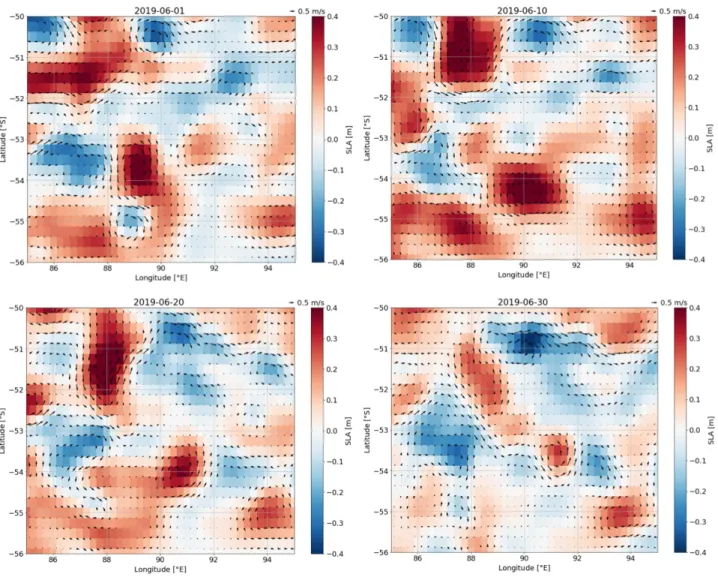
1.8 SLA time evolution . . . 36

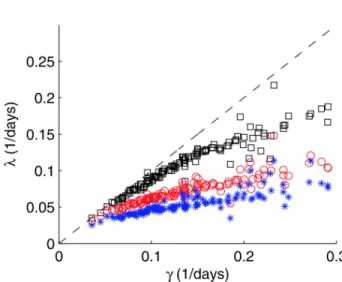
1.9 FTLE versus strain . . . 37

1.10 FSLE snaphot . . . 38

1.11 Surface current speed in LLC4320 . . . 40

2.1 Vorticity conservation . . . 45

2.2 Ertel PV decomposition . . . 46

2.3 Time series of Ertel PV . . . 47

2.4 Geostrophic streamfunction . . . 49

2.5 Okubo-Weiss quantity . . . 50

2.6 Vortex stripping . . . 51

2.7 Ageostrophic circulation schematic . . . 53

2.8 Deformation vs vertical velocity schematic . . . 54

2.9 Boussinesq vs QG flows . . . 56

2.10 Ageostrophic streamfunction . . . 58

5.1 FSLE and Ertel PV . . . 124

5.2 Wavenumber-frequency spectrum . . . 125

5.3 Seismic reflection profiling . . . 127

List of Tables

1 LLC spin-up hierarchy . . . 39

Publications associated with this dissertation

Ageostrophic dynamics

• Siegelman, L., Klein, P., Rivière, P., Thompson. A.F., Torres, H.S., Flexas, M. and Menemenlis, D. (2020). Enhanced upward heat transport at deep submesoscale ocean fronts. Nature Geoscience, 13(1), 50-55. (Chapter 3)

• Siegelman, L.. (2020). Energetic submesoscale dynamics in the ocean interior. Journal of Physical Oceanography, 50(3), 727-749. (Chapter 4)

• Siegelman, L., Klein, P., Torres, H., Thompson, A.F. and Menemenlis, D. (2020). Altimetry-based diagnosis of deep-reaching submesoscale ocean fronts. Fluids, 5(3), 145.

• Archer, M., Schaeffer, A., Keating, S., Roughan, M., Holmes, R. and Siegelman, L. (2020). Observations of submesoscale instability and frontal subduction within the mesoscale eddy field of the Tasman Sea. Journal of Physical Oceanography, 50(5), 1509-1529.

Biological impact of ageostrophic dynamics

• Siegelman, L., O’Toole, M., Flexas, M., Rivière, P. and Klein, P. (2019). Submesoscale ocean fronts act as biological hotspot for southern elephant seal. Scientific reports, 9(1), 2045-2322. (Chapter 5)

• Rivière, P., Jaud, T., Siegelman, L., Klein, P., Cotté, C., LeSommer, J., Dencausse, G. and Guinet, C. (2019). Sub-mesoscale fronts modify elephant seals foraging behavior. Limnology and Oceanography Letters, 4(6), 193-204.

Data processing

• Siegelman, L., Roquet, F., Mensah, V., Rivière, P., Pauthenet, E., Picard, B. and Guinet, C. (2019). Correction and accuracy of high-and low-resolution ctd data from animal-borne instruments. Journal of Atmospheric and Oceanic Technology, 36(5), 745-760. (Chapter 1.1)

• Mensah, V., Roquet, F., Siegelman, L., Picard, B., Pauthenet, E. and Guinet, C. (2018). A correction for the thermal mass–induced errors of CTD tags mounted on marine mammals. Journal of atmospheric and oceanic technology, 35(6), 1237-1252.

• Manucharyan, G., Siegelman, L. and Klein, P. (in revision). State estimation of surface and deep flows from sparse SSH observations of geostrophic ocean turbulence using Deep Learning. Journal of Advances in Modeling Earth Systems.

Balanced motions and internal gravity waves from space

• Klein, P., Lapeyre, G., Siegelman, L., Qiu, B., Fu, L.L., Torres, H.S., Su, Z., Menemenlis, D. and Le Gentil, S. (2019). Ocean-scale interactions from space. Earth and Space Science, 6(5), 795-817. (Appendix A)

• Torres, H.S., Klein, P., Siegelman, L., Qiu, B., Chen, S., Ubelman, C., Wang, J., Menemenlis, D. and Fu, L.L. (2019). Diagnosing ocean-wave-turbulence interactions from space. Geophysical Research Letters., 46(15), 8933-8942. (Appendix B)

Scientific activity during the PhD

Field work

• Kerguelen Islands, French Antarctic and Southern territories Nov 2016–Feb 2017 Program 109 IPEV, PI: C. Guinet. Data acquisition for the PhD. Southern elephant seal CTD-SRDL tag deployment and retrieval.

International collaborations

• Jet Propulsion Laboratory, California Institute of Technology 2017–2019 NASA JPL Visiting Student Research Program in Lee-Lueng Fu’s general ocean circulation group.

• California Institute of Technology 2017–2019

Visiting Graduate Student in Andrew F. Thompson’s physical oceanography research group.

Teaching

• Université de Bretagne Occidentale Sep–Dec 2017

Teaching assistant. General physics, freshman year, 60 hours.

International Meetings

• AOGS Asia Oceania Geosciences Society Meeting, Singapore 2019 Deep submesoscales: elephant seal and satellite unravel a major pathway connecting the ocean interior to the surface (presentation).

• AOFD Atmospheric and Oceanic Fluid Dynamics Meeting, Portland, ME 2019 Enhanced heat transport at deep ageostrophic ocean fronts (presentation).

• SWOT Science Team Meeting, Bordeaux, France 2019

Elephant seal and satellite provide insight towards reconstructing vertical velocities at submesoscale from space (presentation).

• Ocean Sciences Meeting, Portland, OR 2018

Mesoscale and sub-mesoscale dynamics in the Kerguelen region, Southern Ocean, revealed by Southern Elephant Seals (poster).

Introduction

Context

The ocean is the largest solar energy collector on Earth. It absorbs about 90% of Earth’s radiation

imbalance (Hansen et al., 2011) and, as such, plays a crucial role in the regulation of our climate. The

amount of heat the ocean can store is modulated by its complex circulation, which spans a broad range

of spatial scales, from centimeters to thousands of kilometers. This dissertation focuses on the scale

range 1–500 km, which encompasses two major physical structures: mesoscale eddies (100–300 km size),

Figure 0.1:

Visible Infrared Imaging Radiometer Suite on the Suomi satellite captures an extensive phytoplankton bloom just west of the Drake Passage, one of the most turbulent regions in the ocean. Mesoscale eddies and submesoscales filaments are noticeable on this image. From https://earthobservatory. nasa.gov.

which account for most of the oceanic

Kinetic Energy (KE), and

subme-soscale fronts (

_{≤ 50 km size), which}

capture most of the vertical velocity

field.

Satellite altimetry of the past

twenty-five years has revealed the existence of

a strongly energetic mesoscale

turbu-lent flow field in all the oceans (Klein

et al., 2019).

This oceanic mesoscale

turbulence is characterized by cyclonic

and anticyclonic eddies with an

hori-zontal length scale of 100–300 km, a

vertical length scale of 500–1000 m and

a time scale ranging from a few days

to several weeks (Chelton et al., 2011).

At leading order, mesoscale eddies are

in geostrophic balance, i.e., a balance

between pressure and Coriolis forces.

They are mostly energetic in turbulent

regions such as the Gulf Stream, the

Kuroshio Extension, and the Antarctic Circumpolar Current (Figures 0.1 and 0.2).

Figure 0.2:

Surface relative vorticity in the Kuroshio Extension on March 15th 2002 from a high-resolution (1/30◦in the horizontal and 100 vertical levels) numerical simulation of the North Pacific using the ocean general circulation model for the Earth Simulator. From Sasaki et al. (2014).

Mesoscale eddies account for

_{∼ 80% of the total oceanic KE (Ferrari and Wunsch, 2009). In terms of}

KE budget, numerical and theoretical studies indicate that mesoscale eddies experience an inverse KE

cascade, with KE fluxing from the source (

_{∼ 50–100 km), resulting from the baroclinic instability of}

large-scale currents, towards larger scales (Tulloch et al., 2011; Klein et al., 2019). In simple terms, this

happens when two small eddies merge to form a larger one. This inverse KE cascade increases the total

eddy KE and strengthens large geostrophic eddies as they become more coherent and their life time

increases (Arbic et al., 2012; Qiu et al., 2014; Sasaki et al., 2014). Mesoscale eddies are a key component

of the global ocean circulation and significantly impact, among others, carbon sequestration, biological

productivity, heat transport and thus the Earth’s climate as a whole (Ferrari and Wunsch, 2009).

However, a new vision of ocean dynamics has emerged in the last two decades. It highlights the

previ-ously unsuspected importance of submesoscale motions, confined within the ocean surface mixed layer,

for the general ocean circulation (Spall and Richards, 2000; Lévy et al., 2001). Submesoscales have an

horizontal length scale

_{≤ 50 km and a time scale ranging from hours to days. They lie intermediate to}

meso- and small-scale 3-D (0.1–100 m) motions and take the form of elongated fronts or filaments

embed-ded within mesoscale eddies (Figures 0.1 and 0.2). Contrary to mesoscale eddies, submesoscale motions

are not in geostrophic balance (Thomas et al., 2008), as such they are referred to as "ageostrophic"

motions.

While mesoscales capture most of the horizontal eddy KE (u, v), submesoscales capture most of the

vertical eddy KE (w) (Klein and Lapeyre, 2009; McWilliams, 2016), as illustrated in Figure 0.3. This

figure shows that while most of the variance of

(u, v) lies in the mesoscales, most of the variance of w is

contained at submesoscales. Submesoscale dynamics are known to generate vertical velocities of

_∼100

m/day that are typically an order of magnitude larger than those associated with the mesoscale. As

such, submesoscale dynamics play an important role in the vertical transport of key properties such as

climatically important gazes, heat and nutrient (Klein and Lapeyre, 2009; Ferrari, 2011).

Figure 0.3:

a) Vertical velocity and b) horizontal velocity at a 200-m depth as a function of the length scale for mesoscales (blue line) and submesoscales (red line), assuming equal KE for both regimes at the length scale of 100 km. From Klein and Lapeyre (2009).

To date, submesoscale dynamics have mainly been studied in the upper ocean, and in particular within

the ocean mixed layer (

_{∼50–100 m deep), where they are thought to be dominant due to the presence}

of horizontal density gradients, vertical shear, weak stratification, and a surface boundary conducive

to frontogenesis. In contrast, submesoscales in the ocean interior are currently assumed to be weak.

This is because the ocean interior is commonly assumed to be in geostrophic balance, preventing the

formation of strong horizontal gradients. However, growing evidence suggests that the interior ocean

may depart from geostrophy and host energetic submesoscales. For instance, this has been proposed

by Molemaker et al. (2010) in an idealized study, in which the authors demonstrate the presence of

energetic frontogenesis driven by mesoscale eddies in the ocean interior. Seismic imaging has also long

revealed the existence of energetic eddies in the ocean interior (Biescas et al., 2008; Menesguen et al.,

2009; Barbosa Aguiar et al., 2015), such as the subsurface anticyclones of the North Atlantic known as

"meddies" (Armi et al., 1988; Ménesguen et al., 2012) or the coherent eddies of the Gulf Stream (Gula

et al., 2019). In addition, the recent in situ study of Yu et al. (2019) diagnosed strong upward vertical

heat fluxes in the ocean interior that are believed to be produced by submesoscale dynamics.

Furthermore, mesoscale and submesoscale dynamics are often studied independently. To date, only a

few studies (Fox-Kemper and Menemenlis, 2008; Klein and Lapeyre, 2009; Tulloch and Smith, 2009)

have examined their interactions beyond the dynamics of stable/unstable submesoscale fronts embedded

in a large-scale strain field. This dissertation addresses the question of the two-way interaction between

mesoscale eddies and submesoscale structures in a fully turbulent flow field. More precisely, the focus

of this work is on ageostrophic dynamics (see Chapter 2 for the precise definition) in the ocean interior,

and in particular below the mixed layer, where little is known about their existence. The main purposes

of this work are to show that ageostrophic motions (i) are generated by the backgound mesoscale eddy

field via frontogenesis processes, and (ii) are not solely confined to the ocean surface mixed layer but,

rather, can extend in the ocean interior down to depths of a thousand meters. As such, submesoscale

fronts provide an important, yet unexplored, pathway for the transport of heat, chemical and biological

tracers, between the ocean interior and the surface, with potential major implications for the

biogeo-chemical and climate systems.

This dissertation focuses on one of the most energetic regions of the world’s ocean: the Antarctic

Circumpolar Current (ACC) (Hogg et al., 2015), from which numerous eddies emanates, making it

prone to the generation of submesoscale motions. This region has been chosen because of availability of

two groundbreaking datasets: (i) submesoscale-resolving in situ observations collected by instrumented

elephant seals in the Kerguelen area (Indian sector of the Southern Ocean, Figure 1.2) and (ii) outputs

from a realistic simulation at high-resolution that includes internal tides. In addition, this region benefits

from a thorough satellite altimetry coverage, allowing to access the mesoscale activity of the area. As

such, the availability of these three independent datasets enabled the study of ageostrophic dynamics

in the ocean interior from an observational and modeling perspective.

Outline

• Chapter 1 describes the three datasets used in this dissertation:

– Conductivity-Temperature-Depth data collected by instrumented southern elephant seals in

the Kerguelen area (Figure 1.2), providing vertical sections of density at high-resolution,

capable to resolve agoestrophic dynamics at depth.

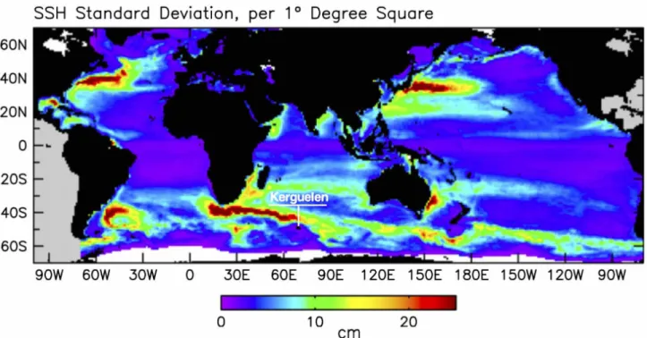
– Conventional satellite altimetry data, providing maps of sea surface height (SSH), a proxy for

surface pressure, sufficient to resolve the mesoscale activity of the area. Finite size Lyapunov

exponents are subsequently computed from SSH to retrieve the strain field.

– A global and realistic numerical simulation with a 1/48

◦

horizontal resolution, 90 vertical

levels and tidal forcing, i.e., the so-called LLC4320 simulation.

• Chapter 2 introduces the theoretical concepts related to quasi-geostrophic and ageostrophic

dy-namics that will be used in Chapters 3–5. The aim of this chapter is to summarize the key

theoretical results related to meso- and submesoscale turbulence. This chapter can be read

inde-pendently from the others.

• Chapter 3 demonstrates the existence of submesoscale fronts in the ocean interior. These fronts

generate enhanced upward vertical heat transport at depth. The results are based on an innovative

methodology combining seal and satellite data, and are backed by an analysis of the high-resolution

numerical simulation.

• Chapter 4 is in the continuity of Chapter 3; it confirms the presence of ageostrophic dynamics

in the ocean interior and proposes a dynamical explanation for it, based on an analysis of the

high-resolution numerical simulation.

• Chapter 5 presents a biological impact of ageostrophic dynamics for a top predator; the southern

elephant seal. Its foraging activity is shown to be stimulated in the vicinity of submesoscale fronts.

• Lastly, the main results of this dissertation are summarized and some perspectives on questions

that will need to be addressed in future work are presented.

1

Datasets

Three main datasets are used in this dissertation thesis; high-resolution observations collected by

instru-mented elephant seals in the Kerguelen area, satellite altimetry data, from which finite-size Lyapunov

exponents are derived, and outputs from a realistic numerical simulation at high-resolution. The

com-bination of the first two independent datasets (seal and satellite data) provides a synoptic 3-D view of

the upper ocean, down to depths of

_{∼ 500 m (Figure 1.1). The numerical simulation is then used to}

confront and extend the observational results to the first thousand meters of the water column.

Figure 1.1:

Schematic view of the upper 500 m of the ocean in the Kerguelen area (Indian sector of the Southern Ocean, see white polygon). Elephant seals sample mesoscale eddies. They are localized by the Argos satellite system (satellite on the left). Their dive trajectory is shown by the dashed curve. Satellite altimeter diagnoses sea surface height (satellite on the right). c _{Tandi Reason Dahl.}

1.1

High-resolution observations collected by instrumented southern elephant seals

Hydrographic data collected by marine mammals such as Southern Elephant Seals (Mirounga leonina)

represent a consequent source of information, especially in the undersampled polar oceans where

observa-Figure 1.2:

a) Zonal number of profiles from MEOP-CTD (blue), ship-based CTD (red) and ARGO floats (yellow) from the world ocean database 2013 (Boyer et al., 2013). Note the major contribution of MEOP south of 50◦S. b) Density distribution of 529,373 CTD profiles from the MEOP-CTD database. From Pauthenet (2018).

tions are notoriously hard to acquire (Roquet et al., 2014; Treasure et al., 2017) (Figure 1.2). Since 2002,

instrumented animals have been generating large datasets of oceanographic

Conductivity-Temperature-Depth (CTD) casts (> 500 000 profiles), which are freely available to the scientific community through

the Marine Mammals Exploring the Oceans Pole to Pole (MEOP) data portal (http://meop.net).

Us-ing marine mammals as data-collection platform has proved to be a powerful and cost-effective way to

improve the ocean observing system for both physical and biological oceanographers. In fact, over 90%

of CTD profiles south of 60

◦

S have been collected by instrumented marine mammals (Treasure et al.,

2017) (Figure 1.2).

Subantarctic and Antarctic islands, such as the Kerguelen, Macquarie, New South Wales, South

Geor-gia, Bouvet or Falkland Islands, are home to large population of southern elephant seals. The southern

elephant seal is a deep-diving (600

_{± 200 m, with maxima around 2,000 m, Figure 1.3), wide-ranging}

marine predator species. It forages on mesopelagic fish in either one of three main habitats: the

Antarc-tic continental shelf, the Kerguelen Plateau or deep open water regions (Hindell et al., 2016). Southern

elephant seals spend

_{∼ 8 months per year at sea and come back to land twice a year for a cumulative}

period of

_{∼ 4 months; once to moult and once to breed.}

Figure 1.3:

Colony of southern elephant seals at Kerguelen Islands during the molting season in December 2016, with an instrumented female in the background (white circle). Find out more about it in the NASA news release at https://www.jpl.nasa.gov/news/news.php?feature=7392. Picture c _{Etienne Pauthenet, Sorbonne} Université. The inset shows the trajectory of a southern elephant seal, with temperature profiles reaching depths of_{∼ 1000 m. c Thomas Jaud.}

Figure 1.4:

Photograph of a CTD-SRDL, with visible hardware compo-nents labeled. The miniaturized CTD unit samples the water column during the ascent phase of the seal’s dive. Data are then transmitted via the satellite transmission system Argos. From Trea-sure et al. (2017).

When they come back to land, elephant seals are equipped

with CTD–Satellite Relay Data Logger (CTD-SRDL) tags

(Figure 1.4), that are either retrieved at the end of the

de-ployment or fall off with the animal’s dead skin during the

next moulting season.

CTD-SRDLs are built by the Sea

Mammal Research Unit at the University of St Andrews in

Scotland and incorporate a miniaturized CTD unit

manufac-tured by Valeport Ltd. (Boehme et al., 2009). They record

conductivity, temperature and pressure, from which salinity

and, then, density are derived (Figure 1.4). In addition, the

seal’s geographic position is tracked via the Argos satellite

sys-tem.

The data is traditionally compressed before being sent via Argos, due to limited battery and bandwidth

capabilities. Approximately 5 profiles, made of

_{∼15 points each, are sent per day (Roquet et al., 2011).}

However, thanks to recent improvements in battery capacity, a handful of CTD-SRDL have been set in

continuous recording mode at the sampling frequency of 0.5 Hz, recording every dive realized by a seal

during its journey. Since elephant seals typically perform more than 80 dives per day, this gives access

to the density field at high-resolution over periods of several months, opening new horizons for the study

of submesoscale physics in eddy-rich regions of the world oceans. Since 2014, twenty-eight such tags

have been deployed at the Kerguelen Islands (French Southern Territories, Figure 1.2) and at Peninsula

Valdes (Argentina) as part of the SO-MEMO program led by Christophe Guinet (CEBC/CNRS, France).

However, to be fitted on marine mammals, the tags are considerably smaller than a traditional CTD

and often contain residual noise related to the miniaturized sensors capabilities (Roquet et al., 2017).

Raw temperature and conductivity data are affected by a thermal lag effect, particularly pronounced

across sharp thermoclines, and especially apparent on high-resolution profiles. Thus, we implemented

an post-processing procedure aimed at improving the data quality, described in Siegelman et al. (2019b)

and presented below. We build on papers published by Roquet et al. (2011) and Mensah et al. (2018).

These authors developed initial corrections and accuracy estimates of animal-borne CTD data collected

as part of the international MEOP consortium. Here, we take advantage of the newly available dataset

of high-resolution profiles recorded, in continuous, at the sampling frequency of 0.5 Hz. More precisely,

we make use of 7 tags deployed in the Southern Ocean from 2014 to 2018, allowing to access for the

first time the ascent and descent of a dive. Thanks to this unique dataset, we develop and validate an

autonomous post-processing procedure that considerably improves the quality all CTD-Satellite Relay

Data Logger (CTD-SRDL) data, i.e. both high-resolution profiles recorded at the frequency of 0.5 Hz

and compressed low-resolution ones transmitted in near-real time via satellite. The procedure corrects

for the thermal lag effect on temperature and salinity and, subsequently, removes density inversions by

adjusting salinity while leaving temperature unchanged. Overall, the procedure is applied to over 50 000

profiles (including high- and low-resolution profiles). In the process, we also refined accuracy estimates

of CTD-SDRL data and, in particular, estimated for the first time the compression error associated to

low-resolution data that, to date, represent 95% of the tags logged in the MEOP database. Thanks to

recent progress in the field of bio logging, continuous high-resolution dataset are expected to become

increasingly available. As such, the approaches proposed in this paper should gain increasing utility.

We refer the curious reader to Siegelman et al. (2019b) for technical details related to each tag’s own

characteristics and associated errors. However, briefly, the final used in this dissertation has a

post-correction accuracy of

_±0.02

◦

C for temperature and

_{±0.03 g.kg}

−1

for salinity, a median horizontal

resolution of 700 m, a vertical resolution of 1 m and a mean temporal resolution of 25 min. Note

that this resolution is greater than the one currently obtained from ocean gliders, which typically have

a horizontal resolution of 2–4 km and a temporal resolution of 3–6 hours. In addition, and contrary

to ocean gliders, elephant seals are endurance swimmers that can easily fight the current, painlessly

crossing through, and thus sampling, mesoscale eddies and submesoscale fronts in the energetic ACC.

In Chapter 3, we use of tag 48 deployed in a turbulent mesoscale area east of the Kerguelen Islands and

in Chapter 5, we analyze tag 50 deployed west of the Kerguelen Islands in a less turbulent area (Figure

1.5). Both tags were deployed during the late austral spring–early austral summer of 2014.

Figure 1.5:

Continous CDT-SRDL deployed on 5 southern elephant seals in 2014 at the Kerguelen Islands. The tag number is indicated. Sea level anomaly (sla) from AVISO in shown the background for December 15, 2014. SSH contours corresponding to the Subantarctic (SAF; -0.25 m) and Polar (PF; -0.70 m) fronts are shown in black. Topography contours are plotted in grey.

Correction and Accuracy of High- and Low-Resolution CTD Data from

Animal-Borne Instruments

L

IA

S

IEGELMAN

,

a,b,c

F

ABIEN

R

OQUET

,

d

V

IGAN

M

ENSAH

,

e

P

ASCAL

R

IVIÈRE

,

a

E

TIENNE

P

AUTHENET

,

f

B

APTISTE

P

ICARD

,

gAND

C

HRISTOPHE

G

UINETg

a_{Univ. Brest, CNRS, IRD, Ifremer, LEMAR, Plouzané, France} b

Environmental Science and Engineering, California Institute of Technology, Pasadena, California c

NASA Jet Propulsion Laboratory, California Institute of Technology, Pasadena, California d_{Department of Marine Sciences, University of Gothenburg, Gothenburg, Sweden}

e_{Institute of Low Temperature Science, Hokkaido University, Sapporo, Japan}

f_{Sorbonne Universités, UPMC Univ., Paris 06, UMR 7159, LOCEAN-IPSL, F-75005, Paris, France} g_{Centre d’Études Biologiques de Chizé, CNRS, Villiers-en-Bois, France}

(Manuscript received 28 September 2018, in final form 12 February 2019) ABSTRACT

Most available CTD Satellite Relay Data Logger (CTD-SRDL) profiles are heavily compressed before satellite transmission. High-resolution profiles recorded at the sampling frequency of 0.5 Hz are, however, available upon physical retrieval of the logger. Between 2014 and 2018, several loggers deployed on elephant seals in the Southern Ocean have been set in continuous recording mode, capturing both the ascent and descent for over 60 profiles per day during several months, opening new horizons for the physical oceanog-raphy community. Taking advantage of a new dataset made of seven such loggers, a postprocessing procedure is proposed and validated to improve the quality of all CTD-SRDL data: that is, both high-resolution profiles and compressed low-resolution ones. First, temperature and conductivity are corrected for a thermal mass effect. Then salinity spiking and density inversion are removed by adjusting salinity while leaving temperature unchanged. This method, applied here to more than 50 000 profiles, yields significant and systematic im-provements in both temperature and salinity, particularly in regions of rapid temperature variation. The continuous high-resolution dataset is then used to provide updated accuracy estimates of CTD-SRDL data. For high-resolution data, accuracies are estimated to be of60.028C for temperature and 60.03 g kg21for salinity. For low-resolution data, transmitted data points have similar accuracies; however, reconstructed temperature profiles have a reduced accuracy associated with the vertical interpolation of60.048C and a nearly unchanged salinity accuracy of60.03 g kg21.

1. Introduction

Hydrographic data collected by marine mammals such as southern elephant seals (SES; Mirounga leonina), Steller sea lions (Eumetopias jubatus), or ribbon seals (Histriophoca fascia) equipped with conductivity– temperature–depth Satellite Relay Data Logger (CTD-SRDL) tags (referred to as ‘‘tag’’) represent a consequent

source of information, especially in the undersampled polar oceans where observations are notoriously hard to acquire (Roquet et al. 2014;Treasure et al. 2017). The temperature and conductivity sensors of these tags, manufactured by Valeport, Ltd., yield high precision (60.0058C for temperature and 60.01 ms cm21for con-ductivity; seeBoehme et al. 2009) and reasonable accu-racies (60.028C for temperature and 60.03 g kg21_for

salinity) after delayed-mode calibration (Roquet et al. 2011). However, to be fitted on marine mammals, the tags are considerably smaller than a traditional CTD and often contain residual noise related to the minia-turized sensors capabilities (Roquet et al. 2017). Re-cent studies (Nakanowatari et al. 2017; Mensah et al. 2018) demonstrated that the tags are affected by a ther-mal mass error on their temperature and conductivity cells, particularly pronounced across sharp thermoclines.

Denotes content that is immediately available upon publica-tion as open access.

Supplemental information related to this paper is available at the Journals Online website: https://doi.org/10.1175/JTECH-D-18-0170.s1.

Corresponding author: Lia Siegelman, [email protected]

VOLUME36 J O U R N A L O F A T M O S P H E R I C A N D O C E A N I C T E C H N O L O G Y MAY2019

DOI: 10.1175/JTECH-D-18-0170.1

Correction of the thermal mass–induced error have been proposed and shown to work (Nakanowatari et al. 2017; Mensah et al. 2018) but only for salinity and not for temperature.Mensah et al. (2018)demonstrated that the thermal mass error on salinity is of O(1022) g kg21with maxima of O(1021) g kg21. These authors developed a correction, based onLueck and Picklo (1990), which di-rectly corrects salinity rather than conductivity and yields an error decrease of the salinity measure of up to 50% when using generic parameters values. However, due to the lack of thermal mass correction for temperature, density errors, some of them imputable to temperature, remain.

In addition, some aspects of the accuracy estimates of these data are insufficiently characterized. Indeed, be-sides the calibration errors discussed inRoquet et al. (2011), errors associated with the dynamical response of the tags and the reconstruction of profiles after com-pression also exist but have not been estimated.

In the present paper, we take advantage of a newly available continuous high-resolution dataset (described insection 2c) that advantageously contains the ascend-ing and descendascend-ing phase of dive, allowascend-ing to compare upcasts and downcasts for the first time. This unique dataset is used to tackle all the issues mentioned above, that is, the implementation of a thermal lag correction for temperature and conductivity, incorporation of a salinity correction to remove density inversions, and estimation of the dynamic response error of the tags and of the compression error associated with low-resolution data, all of which contribute to improving the post-processing and accuracy estimates of CTD-SRDL data. Section 2presents the datasets and method employed in this study.Section 3 introduces the correction pro-cedure, which includes preliminary salinity and tem-perature adjustments and the thermal mass correction for conductivity and temperature as well as the density inversion removal algorithm. Section 4 describes the parameter estimation for the thermal mass correction. Section 5presents the correction and accuracy estimates for high-resolution data.Section 6 presents the correc-tion and accuracy estimates for compressed data. A sum-mary and conclusions are proposed insection 7.

2. Datasets and method

a. Satellite-transmitted compressed profile data

Compressed low-resolution profiles are transmitted in near–real time via the Argos satellite system for;4 profiles per day (among the;60 dives per day per-formed by SES) and are typically made of;15 points chosen via a broken-stick point selection algorithm (Boehme et al. 2009). To date, the majority of available

biologged data is made of low-resolution profiles. They represent 85% of the profiles and 95% of the tags in the Marine Mammals Exploring the Oceans Pole to Pole (MEOP) database, which is the largest database of biologged acquired hydrographic data with over 500 000 profiles collected since 2004 (Treasure et al. 2017). In particular, the heavy subsampling associated with the satellite-transmission method of low-resolution data implies the existence of a compression loss that will be evaluated for the first time insection 6c.

The low-resolution dataset employed in this study is made of 43 tags deployed on SES around the Kerguelen Islands from February 2011 to January 2018 (trajectories in black and red in Fig. 1a), amounting to a total of 14 762 CTD profiles. The environment in which SES dived is marked by temperatures of 08–48C, salinities of 34–34.9 g kg21, and densities of 26.9–27.8 kg m23, char-acteristic of the areas north of the polar front (PF), in the Antarctic zone (AAZ), which is defined as the area lo-cated between the PF and the southern Antarctic Cir-cumpolar Current Front (SACCF) and south of the SACCF (Fig. 1).

b. High-resolution profile data from retrieved tags

High-resolution profiles are recorded at the sampling frequency of 0.5 Hz for ;10 profiles per day and are typically made of ;1000 points. However, these data are only available after physical retrieval of the tag due to limited battery capabilities. Thus, compressed pro-files are a subsample of resolution ones. The high-resolution dataset employed in this study corresponds to the high-resolution version of the low-resolution dataset, that is, the same 14 762 dives (trajectories in black and red inFig. 1a) but recorded at the sampling frequency of 0.5 Hz. The high-resolution dataset is used to validate the proposed correction scheme for compressed low-resolution data and to derive the compression error (seesection 6).

c. Continuous high-resolution data

Thanks to recent progress in the field of miniaturiza-tion and satellite telemetry, tags can now record tem-perature, salinity, and pressure at the sampling frequency of 0.5 Hz for every dive of the seal’s journey (.60 dives per day), giving access, for the first time, to both the as-cending and desas-cending phase of a dive. Such tags can last for more than 3 months and cover large oceanic domains at a very high horizontal and vertical resolu-tion (see secresolu-tions of temperature and salinity inFig. 2). These state-of-the-art data are opening new horizons for the physical oceanography community and in par-ticular for the study of small-scale processes of O(1–50) km, also called submesoscales. These submesoscale features,

characterized by elongated fronts and filamentary struc-tures, are now captured by such observations, contrary to previous data obtained from animal-borne CTDs that were either of low resolution or only of high vertical (but not horizontal) resolution. To date, such data have only been briefly introduced inMensah et al. (2018)to vali-date their salinity-based correction. In this paper, we fully exploit the potential of these new data, referred to as the ‘‘continuous high-resolution dataset,’’ that allows for direct comparison of upcasts and downcasts prior to and after correction.

The continuous high-resolution dataset employed in this study is made of seven tags (39 183 profiles) deployed

on SES around the Kerguelen Islands in the Indian Ocean sector of the Southern Ocean from October 2014 to January 2018 (trajectories in red onFig. 1a). The environment in which the SES conducted pro-files is marked by temperatures of 18–58C, salinities of 33.9–34.9 g kg21, and densities of 26.7–27.7 kg m23, characteristic of the area north of the SACCF (see Figs. 1and2).

d. General methodology

In addition to the temperature and salinity adjust-ments introduced inRoquet et al. (2011)and briefly re-called insection 3a, we propose an autonomous two-step

FIG. 1. (a) Spatial distribution of profiles collected by the 43 low-resolution tags (LR; black) among which 7 are also at continuous high resolution (HR; red), deployed from 2011 to 2018 on SES on the Kerguelen Islands. Climatological position of the Subantarctic Front (SAF), Polar Front (PF), Southern Antarctic Circumpolar Current Front (SACCF), and Southern Boundary Front (SBdy) are indicated in blue according toKim and Orsi (2014). (b) Mean conservative temperature (CT) profile of the 43 LR tags (black) and 7 HR tags (red). (c) As in (b), but for absolute salinity (SA). (d) As in (b), but for potential densitys0. In (b)–(d) the 20th and 80th percentiles are shaded.

postprocessing procedure for the correction of MEOP’s profiles also applicable to other hydrographic data acquired via biologging or with unpumped glider. We first implement a correction scheme for the thermal mass effect where temperature (Morison et al. 1994) and conductivity are simultaneously corrected (Lueck and Picklo 1990) instead of only and directly correcting salinity as is done inMensah et al. (2018). This was, however, made possible by the theoretical framework delineated inMensah et al. (2018)(seesections 3band4). We then aim at further refining the salinity correction regarding density inversions, which has not been ad-dressed by previous works and is of particular importance for high-resolution profiles. To do so, hydrographic pro-files are stabilized within the water column by minimally adjusting absolute salinity (SA) while leaving the values of in situ temperature unchanged with the method developed by Barker and McDougall (2017) (see section 3c).

The procedure is applied to the continuous high-resolution dataset as well as to the low-high-resolution dataset introduced in section 2. For high-resolution data, the effect of the correction is documented globally and then separately for the areas north and south of the PF (Fig. 1). The correction is then vali-dated without relying on external data. Indeed, we use the continuous high-resolution dataset that advanta-geously contains both the ascending and descending phase of a dive, to validate the proposed correction by comparing upcast and downcast data before and af-ter correction. Finally, the continuous high-resolution dataset is used to estimate the mean errors associated

with the tag’s dynamical response, which are also esti-mated globally and separately north and south of the PF (seesection 5).

For low-resolution data, the effect of the correction is documented for three oceanic zones: north of the PF, in the AAZ, and south of the SACCF (Fig. 1). The cor-rection is then validated by comparing corrected high-resolution profiles to their low-high-resolution version prior to and after correction. Finally, the compression error associated with low-resolution data is estimated for the first time by comparing corrected low-resolution profiles to their high-resolution counterparts. The com-pression error is derived globally and then separately for the areas north of the PF, in the AAZ, and south of the SACCF (Fig. 1; seesection 6).

Estimation of both the dynamic and compression er-rors enables us to provide updated accuracy estimates for high- and low-resolution data, which should be of prime importance to the physical oceanography community.

3. Correction procedure

a. Step 1: Salinity and temperature adjustments

In this section, we briefly recall the delayed-mode calibration designed by Roquet et al. (2011)and ap-plied to the high- and low-resolution datasets before the correction scheme developed in this study (steps 2 and 3; Fig. 3). Temperature and salinity are first cor-rected for pressure-induced linear biases by comparing CTD-SRDL data to ship-based CTD measurements. An external field effect on the conductivity sensor is also detected, inducing an additional salinity offset.

FIG. 2. Example of 200-km-long section of (a) conservative temperature and (b) absolute salinity at high reso-lution in the Southern Ocean from tag ct112–050–14 (red southwest trajectory from Kerguelen Islands inFig. 1a). The tag recorded information at the sampling frequency of 0.5 Hz from 28 Oct 2014 to 21 Jan 2015, amounting to 6942 dives, or over 80 dives per day, and for a cumulative distance of 5665 km.

This salinity offset is corrected with delayed-mode methods. The first method uses the stable salinity maxi-mum characterizing the Lower Circumpolar Deep Water sampled by the seals foraging south of the SACCF and where this approach is not possible, a statistical method of cross comparison of CTD-SRDL measurements is used. For more details on the delayed-mode calibration methods, we refer the reader toRoquet et al. (2011). Finally, temperature and salinity are vertically in-terpolated onto a regular grid of 1-m resolution.

Note that the two-step correction procedure proposed in this paper can be implemented on hydrographic data acquired via biologging and unpumped glider without requiring step 1, which was specifically designed for the tags manufactured by Valeport, Ltd.

b. Step 2: Thermal mass error

The thermal mass error (TME) is due to the transfer of heat from the sensor’s walls to the sample being measured. This well-documented phenomenon (Lueck 1990) affects the conductivity cells of CTDs, which leads to a significant error in the estimation of salinity. This error is a function of the temperature gradient in space and time and has been widely documented for sharp thermocline (Lueck and Picklo 1990; Morison et al. 1994;Mensah et al. 2009; Liu et al. 2015). The tags considered in this study are particularly affected by the TME on their conductivity cells since they are un-pumped. In addition, it appears that an error in tem-perature also related to the TME exists (Mensah et al. 2018). Building onMensah et al. (2018), who only and directly corrected salinity, we implement a correction scheme for the TME that simultaneously corrects con-ductivity and temperature.

To correct the conductivity measure, we apply the procedure proposed byLueck and Picklo (1990). The thermal mass error is modeled as an initial error aC,

decaying within a relaxation time of 1/b (Lueck 1990). Conductivity is then corrected via

C_T(n)5 G_Ca_C(12 0:5bD_t)21T_hp(n) , (1) with CT the conductivity correction added to the

con-ductivity nth sample, Thp(n) the high-pass-filtered

sam-ple’s temperature, using a first-order discrete-time filter with a time constant t 5 b212 0:5 Dt, n the sample’s

index, GC5 (›C/›T)jS,p the coefficient of sensitivity of

conductivity to temperature at fixed salinity, and pres-sure andDtthe sampling time interval, withDt5 2 s for

CTD-SRDLs. Note that Eq.(1), expressed as inMensah et al. (2018), is equivalent toLueck and Picklo’s (1990) original formulation. Salinity is subsequently derived from the corrected conductivity.

Following Morison et al. (1994), temperature is cor-rected for the TME with a similar scheme according to

T_T(n)5 a_T(12 0:5bD_t)21T_hp(n) , (2) where the only difference with Eq.(1)is the absence of the sensitivity coefficientGC. This second step is

sum-marized in the schematic onFig. 3. Adequate values for the three parameters aT, aC, and b are estimated in section 4.

c. Step 3: Density-inversion removal

Density inversions are commonly contained in ocean-ographic observations and are often due to instrumental noise and phenomena such as salinity spiking. While the

FIG. 3. Schematic summarizing the correction procedure implemented in the MEOP da-tabase. From the raw CTD data, temperature TRawand salinity SRaware first adjusted and vertically interpolated onto a regular grid according to the procedure described inRoquet et al. (2011)(step 1 detailed insection 3a). Then, adjusted conductivity CAdjand temperature TAdjare corrected for the thermal mass error (step 2 detailed insection 3b). Density inversions are then removed by minimally adjusting STMEwhile leaving TTMEunchanged. Finally, a Gaussian filter with a 1-dbar window is applied to TTMEand SDIR(step 3 detailed insection 3c).

TME correction (step 1) suppresses part of this noise, most of the salinity spikes and density inversions persist after its application. Barker and McDougall (2017) propose a method to stabilize hydrographic profiles that removes part of this residual noise. The proce-dure minimally adjusts SA while leaving the values of conservative temperature (CT) unchanged. This den-sity inversion removal (DIR) procedure adjusts the profiles such that they never exceed a minimum N2 threshold (N is the Brunt–Väisälä frequency), set here, and by default, to 13 1029s22. Then a Gaussian filter with a 1-dbar window is applied to CT and SA to re-move sharp and localized jumps induced by the DIR for SA profiles. These jumps occur at a frequency higher than the original sampling frequency and thus are not the reflection of a physical process. Further-more, since experimental noise is observed in CT and in SA, which both contribute to the density estimate, smoothing CT in addition to SA ensures potential density s0 free of density inversion or equivalently

maintains a positive N2. Indeed, N2profiles can exhibit negative values when the filter is only applied to SA but not when it is applied to both SA and CT (not shown). The Gaussian filter also has the advantage to account for the irregular sampling in depth of the raw data that is dependent on the variable vertical speed of the ani-mal. Last, the 1-dbar window does not alter the vertical resolution of the data since the original sampling fre-quency is of 0.5 Hz and the animal ascending speed is between 1 and 2 m s21(Hindell and Lea 1998). This third step is summarized in the schematic onFig. 3.

4. Parameter estimation for the thermal mass

error correction

To achieve an equivalent final salinity correction as the one obtained inMensah et al. (2018), we use their generic parameters values ofb 5 0.06 s21andaS5 0.04.

SinceMensah et al.’s (2018)correction is based on the assumption that the correction of salinity is a linear combination of temperature and conductivity correc-tions, the initial error coefficients aC, aT, and aS are

related byaC5 aT2 aS, whereaSis the initial error for

salinity. The relaxation time 1/b is assumed to be iden-tical for both temperature and conductivity (thus also for salinity).

To derive an optimalaT, we use the continuous

high-resolution dataset mentioned insection 2. The temper-ature correction delineated by Eq.(2)is applied to the ascending and descending phases of every dive ranging from depths of a minimum of 150 m up to 1000 m and occurring within a 10-min interval in order to compare similar water masses, adding up to a total of 32 154 dives.

Differences in temperature between ascent and descent are not only due to the thermal mass effect; changes in the timing and geographic location between both phases actually account for a large part of this difference. How-ever, the temperature difference between ascent and descent caused by natural variability should have no average bias. Consequently, the temperature correc-tion scheme delineated by Eq. (2)is tested through a least squares regression scheme, in which we look for the optimal aT that minimizes the mean bias in

tem-perature

å

400m_z50 B(aT, z) between the ascending phase

of dive i and the descending phase of dive i1 1, where B(a_T, z)5 1 n2 1

å

n21 i51[T aT a (i, z)2 T_daT(i1 1, z)], (3)

with z2 [0, 400] the depth of the measurements (m), i the ith dive, n the number of dives per tag, and TaT

a

and TaT

d the temperature during ascent and descent,

respectively, after application of the temperature cor-rection with the coefficientaT. Note that below 400 m,

Thp is close to 0 such that the impact of the correction

becomes negligible (Fig. 4), which justifies the choice of 400 m in

å

400m_z50 B(aT, z). Note also that we do not use the

same dive for comparing ascending and descending phases but instead compare the ascending phase of dive i to the descending phase of dive i1 1 because SES tend to station at the surface for only a few minutes (;2 min) while they swim underwater for longer periods of time (;25 min). It enables us to minimize the natural vari-ability between ascents and descents.

The test is carried out separately for each of the seven tags, with resulting aT ranging from 0.07 to 0.10 (see

Table S1 in the online supplemental material). An op-timal coefficientaT equal to 0.09 is then defined as the

mean of the sevenaTobtained for each tag. This

opti-malaT coefficient is used to implement the TME

cor-rection for temperature. A value of aC5 aT2 aS5

0:09 2 0:04 5 0:05 is therefore used in combination withb 5 0:06 s21, which produces a salinity correction nearly identical to the one of Mensah et al. (2018). Figure 4presents the mean Thpand temperature bias

averaged for the seven tags. Noticeably, the mean temperature bias before correction is inversely pro-portional to the mean Thp_ascent 2 Thp_descent (black

line), which confirms the appropriateness of the TME correction for the temperature field. Indeed, before correction, the mean temperature bias exhibits a sig-nificant positive (negative) bias between 0 and 200 m (200 and 400 m) (black line inFig. 4b). However, after correction, the mean bias is centered around zero (blue line in Fig. 4b), indicating the suppression of a system-atic bias throughout the water column. More importantly,

between 0 and 400 m, where the impact of the correc-tion is the greatest due to the presence of the strongest Thp, the mean temperature bias is reduced by 75% with

an absolute value of 0.018C before correction and only 0.0038C after correction, which is below the sensor’s precision of60.0058C (Boehme et al. 2009). Besides the averaged impact of the TME correction for tem-perature,Fig. 5apresents a typical ascent and descent profile prior to and after correction. The temperature difference between ascent and descent is reduced by 0.088C at 112 m, a rather considerable improvement. In other words, application of the TME correction to the temperature field successfully removes the mean bias related to the thermal mass effect that is even main-tained within the sensor’s precision of60.0058C.

5. Correction and accuracy of high-resolution

profiles

a. Effect of the correction scheme

Here we only consider the ascending phase of a dive since it is the one retained in the final MEOP database. We use the same continuous high-resolution dataset as insection 4but with no restrictive criteria for depth or time. As a result, the two-step postprocessing correction is now implemented for the 39 183 high-resolution pro-files of the continuous high-resolution dataset.

A typical pre- and postcorrection profile at high res-olution is presented on the top panels ofFig. 6. The

TME (blue curve) first adjusts CT, SA, ands0on a

low-frequency scale of O(100) m. Then salinity spikes and subsequent density inversions occurring at a scale of O(1) m are removed by the DIR (red curve).

Differences between raw and corrected data are computed at both steps and RMS values are presented on Fig. 7. Overall, the largest corrections take place between the surface and 300 m, that is, where stronger gradients of temperature are located (Fig. 4). As ex-pected, the TME has a much larger contribution to the CT correction, whereas both TME and DIR contribute significantly to the correction of SA. Indeed, during the DIR the only effective correction applied to CT is the Gaussian filter. For CT, the root-mean-square (RMS) between raw and corrected data is 5.93 10238C after application of the TME and only 6.1 3 10238C after application of the additional DIR step (Fig. 7a). On the other hand, for SA, the RMS between raw and corrected data is of 2.8 3 1023g kg21 after the TME step and 5.33 1023g kg21 after the DIR. Likewise, fors0, the

RMS is of 2.7 and 4.53 1023kg m23after the TME and DIR, respectively. These results highlight the equally important impact of each step for the correction of SA ands0 (Figs. 6and7). Furthermore, the order of the

steps is important and applying the TME prior to the DIR considerably reduces the amplitude of the DIR (not shown here). In other words, the DIR has a lesser impact on the profiles when applied after the TME than directly on raw data, which points out the contribution

FIG. 4. (a) Mean high-pass filter of temperature Thpduring the ascent (blue line) and descent (red line) and mean Thpascent2 Thpdescent (black line) for the 7 HR tags of the continuous high-resolution dataset used to implement the thermal mass error correction. (b) Mean bias prior to correction (black line) and after correction (blue line) for the 7 HR tags of the continuous high-resolution dataset. The 20th and 80th percentiles are shaded.

of the thermal mass effect correction for reducing den-sity inversions. The mean RMS between raw and cor-rected data is 1.35 3 10228C for CT and 1.17 3 1022g kg21for SA within the upper 300 m. These values are largely above the sensor’s precision, and underscore the relative importance of the correction.

The impact of the correction for high-resolution pro-files is now documented for two zones of the Southern Ocean: north and south of the PF, following the clima-tological definition of Kim and Orsi (2014). Unfortu-nately, the continuous high-resolution dataset used in this study does not contain enough profiles south of the SACCF (191 profiles or ,0.05% of the dataset) to compute separate statistics for the AAZ and the area south of the SACCF. North of the PF, the profiles are marked by a mean temperature and salinity of 2.508C and of 34.42 g kg21, while south of the PF, the means are of 2.018C for temperature and 34.57 g kg21 for salinity

(Table 1). RMSs between raw and corrected data are presented per area and depth range inTable 1. While below 300 m, the impact of correction is equivalent north and south of the PF, it differs between 0 and 300 m, where the correction is stronger by;20% south of the PF for both CT, SA, ands0. For CT, the mean RMS is 1.43

10228C north of the PF and 1.6 3 10228C south of the PF. For SA, the mean RMS is 1.13 1022g kg21north of the PF and 1.33 1022g kg21 south of the PF. Fors0, it is

93 1023kg m23north of the PF and 1.13 1022kg m23 south of it (Table 1).

b. Validation of the correction scheme for

high-resolution profiles

Following the same methodology as insection 4, the two-step correction is applied to the ascending and descending phases of the 39 183 dives that are deeper than 150 m and occur within a 10-min interval, which

FIG. 5. Typical ascent (blue line) and descent (red line) profiles prior to correction (dashed line) and after correction (solid line), zoomed from 0 to 500 m. (a) Conservative temperature. (b) Absolute salinity. (c) Potential density. (d) CT–SA diagram.

amounts to 32 154 dives. Comparison between the as-cending phase of dive i and the desas-cending phase of dive i1 1 is done before correction as well as at both steps of the procedure. For each tag, the RMS error of ascend versus descend is calculated at each depth z according to RMS(z)5 ffiffiffiffiffiffiffiffiffiffiffiffiffiffiffiffiffiffiffiffiffiffiffiffiffiffiffiffiffiffiffiffiffiffiffiffiffiffiffiffiffiffiffiffiffiffiffiffiffiffiffiffiffiffiffiffiffiffiffiffiffiffiffiffiffiffiffiffiffi 1 n2 1

å

n21 i51[Xa(z, i)2 Xd(z, i1 1)] 2 s , (4) with n the total number of dives per tag, Xaand Xdthe

field (CT, SA, orr0) during the ascent and descent,

respectively. This RMS is calculated for the uncor-rected (RMSraw) and corrected (RMScor) CT, SA, and

r0at the TME and DIR steps. The performance of the

correction is then evaluated through the difference Dcor5 RMSraw2 RMScorat both steps, with positive

values indicating a decrease of the RMS error due to a convergence of ascending and descending profiles post correction. All seven tags see a continuous and significant improvement at each step of the procedure for all three fields. The difference between the as-cending and desas-cending phases for both CT, SA, and s0is reduced after correction, as can be inferred from

FIG. 6. Typical profile undergoing the correction scheme. High-resolution profiles of (a)–(c) conservative temperature, absolute salinity, and potential density, respectively. (d)–(f) As in (a)–(c), respectively, but showing low-resolution profiles.

the positive Dcorpresented on the upper panels ofFig. 8,

even though between 200 and 400 m the difference is slightly negative for CT (but inferior to the sensor’s pre-cision). The TME reduces most the difference between ascents and descents for CT with meanjDcorj over the

water column of 1.33 10238C at both steps. For SA and s0, the two steps incrementally contribute to reduce the

difference between ascents and descents with a mean jDcorj of 1.5 and 3.0 3 1023g kg21for SA at step TME

and DIR, respectively, and 1.4 and 2.93 1023kg m23for s0at step TME and DIR, respectively.

Overall, the error difference Dcoris most reduced in

areas of strong temperature gradients, that is, between the surface and 300-m depth (Figs. 4and8), which itself

coincides with the strongest impact of the correction procedure (Fig. 7), emphasizing the procedure’s effi-ciency. Besides the effect of the correction scheme presented on Fig. 8over the entire water column, a typical pre- and postcorrection profile, between the surface and 300 m, is shown onFig. 5. The profile, which occurs in a region presenting sharp temperature vari-ations and thus particularly prone to thermal mass and salinity spiking effects, sees its temperature difference between ascent and descent reduced by 83 10228C at 112 m and its salinity by 43 1022g kg21at 130 m, two rather considerable improvements which are also re-flected on the density profile (Fig. 5c) and in the TS plan (Fig. 5d).

FIG. 7. Mean RMS between raw and corrected data for (top) the 7 HR tags for (a) CT, (b) SA, and (c)s0and (bottom) the 43 LR tags for (d) CT, (e) SA, and (f)s0. The 20th and 80th percentiles are shaded.

c. Accuracy estimates

Besides calibration errors discussed inRoquet et al. (2011)and estimated to be of60.028C for temperature and 60.03 g kg21 for salinity after delayed-mode cali-bration, the tags are also subject to a thermal lag re-sponse as documented in this study as well as in previous works (Nakanowatari et al. 2017;Mensah et al. 2018). Even after correction, a residual error imputable to thermal lag effects remains. In this section, we quantify this dynamical bias present in CTD-SRDL data, and also detail it north and south of the PF.

The mean dynamical error is estimated from the continuous high-resolution dataset through the calcu-lation of B(aT, z) defined by Eq.(3)after application of

the two-step correction. Results are presented for the entire water column on the top panels of Fig. 9 and summary statistics per zone can be found inTable 1, in which the mean dynamical error over the water column is defined by M_z max5 1 z_max

å

z_max z50jB(aT, z)j, (5)

where zmaxis the maximal depth, here, 1000 m. For both

CT and SA, the mean dynamical bias M1000 is of 2.73

10238C and 4.1 3 1023g kg21, respectively, which is well below the sensor’s accuracies of60.0058C for temper-ature and60.02 g kg21for salinity. The s0 also has a

weak mean bias with a value of 3.53 1023kg m23. For all three quantities M1000is larger north than south of the

PF by 75% for CT and 50% for SA ands0. Furthermore,

across all areas, the mean dynamical bias is larger in the first 300 m by 45% for CT and 25% for SA ands0.

In conclusion, application of the TME and DIR con-siderably improves the final accuracy of CTD-SRDL data, with mean dynamical errors estimated to be below

the sensor’s precision of 60.0058C for temperature and60.02 g kg21 for salinity. This means that after application of the correction procedure, dynamical errors are negligible compared to calibration errors such that the accuracies of 60.028C for temperature and60.03 g kg21for salinity presented inRoquet et al. (2011)are still valid for high-resolution data.

6. Correction and accuracy of compressed profiles

a. Effect of the correction scheme

The low-resolution version of the high-resolution profile shown on Fig. 6a is presented on the bottom panels of the same figure. Overall, the correction pro-cedure behaves similarly but with a few noticeable differences. Similarly to the high-resolution profile, CT is primarily affected by the TME. However, for SA and s0, only the effect of the TME is large while that of DIR

has become insignificant. As mentioned before, the TME acts on scales of O(100) m while the DIR tends to act on scales of O(1) m. The strong (weak) impact of the TME (DIR) is thus consistent with the low reso-lution of the profile that does not have enough data points to generate salinity spiking. In addition, the Gaussian filter has a negligible impact for all three quantities (not shown), which is also coherent with the low resolution of the profile.

These observations can be generalized to the entire dataset and the application of the correction procedure to the 14 762 low-resolution profiles yields similar re-sults as for high-resolution ones (Fig. 7, lower panels). The shape of the correction’s impact within the water column is preserved, with the strongest corrections occurring once again between the surface and 300-m depth. However, as mentioned before, the TME now has the main impact for CT, SA, ands0 with a mean

TABLE1. Statistics relative to high-resolution (HR) data per oceanic zone and depth range averaged for the seven tags of the continuous HR dataset used in this study. Mean CT, SA, and RMS between raw and final profiles are presented, as is the mean error bias defined by Eq.(5), for which 14 904 profiles are used north of the PF and 17 250 south of the PF, adding to a total of 32 154 profiles. The location of the PF is defined according toKim and Orsi (2014).

Zone No. of HR profiles Depth (m) CT (8C) SA (g kg21) RMS of CT (8C) RMS of SA (g kg21) RMS ofs0 (kg m23) CT mean bias (8C) SA mean bias (g kg21) s0mean bias (kg m23) North of PF 17 592 0–300 2.64 34.04 0.014 0.011 0.009 0.004 0.005 0.005 300–1000 2.45 34.58 0.003 0.003 0.002 0.003 0.004 0.004 0–1000 2.50 34.42 0.006 0.006 0.004 0.003 0.005 0.004 South of PF 21 591 0–300 1.66 34.20 0.016 0.013 0.011 0.003 0.004 0.004 300–1000 2.17 34.73 0.003 0.002 0.002 0.001 0.002 0.002 0–1000 2.01 34.57 0.007 0.007 0.005 0.002 0.003 0.003 All 39 183 0–300 2.38 34.10 0.014 0.012 0.010 0.003 0.005 0.004 300–1000 2.36 34.63 0.003 0.003 0.002 0.002 0.004 0.003 0–1000 2.36 34.47 0.006 0.006 0.004 0.003 0.004 0.003 MAY2019 S I E G E L M A N E T A L .

755

RMS between raw and corrected data of 4.9 and 4.5 3 10238C for CT at step TME and DIR, respectively, 2.3 and 3.03 1023g kg21for SA, and 2.3 and 2.73 1023kg m23 for s0. Once again, the correction is noticeably stronger

between 0 and 300 m with average RMS between raw and final data of 11.93 10238C for CT, 7.1 3 1023g kg23for SA, and 6.63 1023kg m23fors0.

As for the high-resolution profiles, a regional analysis is conducted on the low-resolution dataset. Since a large amount of profiles are located south of the SACCF (5438 profiles or 37% of the dataset), three zones are now an-alyzed: the area north of the PF, the AAZ, and the area south of the SACCF, where the fronts are also defined according to Kim and Orsi (2014). Mean temperatures

are 2.778, 2.178, and 0.848C and mean salinities 34.43, 34.52, and 34.62 g kg21 for the areas north of the PF, in the AAZ, and south of the SACCF, respectively. The temperature correction is equivalent in all three zones regardless of the depth range. For SA and s0,

the correction is equivalent in the three zones below 300 m but in the upper 300 m it is more important south of the PF (in both the AAZ and the area south of the SACCF), as for to the correction impact on high-resolution data. For SA, the mean RMS is 0.005 g kg21north of the PF and 0.007 and 0.008 g kg21 in the AAZ and south of the SACCF, respectively. For s0, it is 0.005 kg m23north of the PF and 0.007 kg m23

south of it (Table 2).

FIG. 8. Mean RMS difference between ascending and descending phases of a dive at each step of the correction procedure for (top) the 7 HR tags for (a) CT, (b) SA, and c)s0and (bottom) the 43 LR tags for (d) CT, (e) SA, and (f)s0. The 20th and 80th percentiles are shaded.