HAL Id: inria-00371193
https://hal.inria.fr/inria-00371193
Submitted on 31 Mar 2009
HAL is a multi-disciplinary open access
archive for the deposit and dissemination of
sci-entific research documents, whether they are
pub-lished or not. The documents may come from
teaching and research institutions in France or
abroad, or from public or private research centers.
L’archive ouverte pluridisciplinaire HAL, est
destinée au dépôt et à la diffusion de documents
scientifiques de niveau recherche, publiés ou non,
émanant des établissements d’enseignement et de
recherche français ou étrangers, des laboratoires
publics ou privés.
and Generators
Laszlo Szathmary, Petko Valtchev, Amedeo Napoli
To cite this version:
Laszlo Szathmary, Petko Valtchev, Amedeo Napoli. Efficient Vertical Mining of Frequent Closed
Itemsets and Generators. [Research Report] 2009, pp.16. �inria-00371193�
Frequent Closed Itemsets and Generators
Laszlo Szathmary1, Petko Valtchev1, and Amedeo Napoli2
1 Dépt. d’Informatique UQAM, C.P. 8888,
Succ. Centre-Ville, Montréal H3C 3P8, Canada [email protected], [email protected]
2 LORIA UMR 7503, B.P. 239, 54506 Vandœuvre-lès-Nancy Cedex, France
Abstract. The effective construction of many association rule bases re-quire the computation of both frequent closed and frequent generator itemsets (FCIs/FGs). However, these two tasks are rarely combined. Most of the existing solutions apply levelwise breadth-first traversal, though depth-first traversal is knowingly superior. Hence, we address here the depth-first FCI/FG-mining. The proposed algorithm, Touch, deals with both tasks separately, i.e., uses a well-known vertical method, Charm, to extract FCIs and a novel one called Talky-G, to extract FGs. The respective outputs are matched in a post-processing step. Experi-mental results indicate that Touch is highly efficient and outperforms its levelwise competitors.
1
Introduction
The discovery of meaningful associations is a key data mining discipline [1]. An association miner typically proceeds in two steps: (i) extract all frequent patterns X of a database, and (ii) break each X into a premise Y , and a conclusion X \Y parts to form a rule Y → X \ Y . Interestingness measures, such as support and confidence, are applied to prune the set of extracted association rules. However, the number of the remaining rules may still be way too high to be practical. As a remedy, various concise representations of the family of valid association rules have been proposed [2,3,4], whereas others have been imported from related fields such as concept analysis [5,6]. A good survey can be found in [7].
Here we focus on the computation of FCIs and FGs, on which are based the minimal non-redundant association rules (MN R) for instance. Following [2], these are rules with the form P → Q \ P , where P ⊂ Q, P is a (minimal) generator (a.k.a. key-sets or free-sets) and Q is a closed itemset. In other terms, in such rules the premise is minimal and the conclusion is maximal. As shown in [7], MN R is a lossless, sound, and informative representation of all valid rules. Moreover, further restrictions can be imposed on the rules in MN R, leading to more compact representations such as the generic basis or the proper basis (see [7] for a complete list).
From a computational point of view, constructing MN R or its sub-structures requires the family of frequent closed itemsets (FCIs) and their generators (FGs), and possibly the precedence order between FCIs. A few methods for extracting both FCIs and FGs have been published in the mining literature, e.g. A-Close [8] or Titanic [9]. Generators have been targeted within the concept analysis field as well [10], e.g. by the Zart algorithm [11]. Well-known FCI/FG-miners exclusively apply levelwise strategies, although the levelwise itemset miners are knowingly outperformed by depth-first methods (e.g. Charm [12] and Closet [13]) on a broad range of dataset profiles, especially on dense ones. Hence the idea of de-signing a depth-first FCI/FG-miner. The presented algorithm called Touch splits the FCI/FG-mining task into its components and solves them separately. The first one by applying Charm and the second one through an original method for FG-mining, the Talky-G algorithm. In an efficient post-processing step, Touch associates the FGs to their respective FCIs, thus providing the necessary start-ing point for the production of MN R. Experimental results show that Touch outperforms two other efficient competitors, A-Close [8] and Zart [11], espe-cially on dense and highly correlated datasets. Thus, the contributions of our study lay mainly in the design of an efficient method, Touch, for constructing the aforementioned rule bases. Additionally, Talky-G is a stand-alone algorithm for extracting FGs.
The paper is organized as follows. Section 2 provides the basic concepts of frequent itemset mining. In Section 3, we give an overview of vertical depth-first algorithms such as Eclat and Charm. In Section 4, we introduce a new FG-miner algorithm called Talky-G. The Touch algorithm that combines the results of Charm and Talky-G is introduced in Section 5. Finally, conclusions and future work are discussed in Section 6.
2
Basic Concepts
Consider the following 5 × 5 sample dataset: D = {(1, ACDE), (2, ABCDE), (3, AB), (4, D), (5, B)}. Throughout the paper, we will refer to this example as “dataset D”.
We consider a set of objects or transactions O = {o1, o2, . . . , om}, a set of
at-tributesor items A = {a1, a2, . . . , an}, and a relation R ⊆ O × A. A set of items
is called an itemset. Each transaction has a unique identifier (tid), and a set of transactions is called a tidset.3
For an itemset X, we denote its corresponding tidset, often called its image, as t(X). For instance, in dataset D, the image of AB is 23 (t(AB) = 23). Conversely, i(Y ) is the itemset corresponding to a tidset Y . The length of an itemset is its cardinality, whereas an itemset of length i is called an i-itemset. The (absolute) support of an itemset X, denoted by supp(X), is the size of its image, i.e. supp(X) = |t(X)|. The image function induces an equivalence relation on the power-set of items ℘(A): two itemsets are equivalent
3
if they share the same image (X ∼= Z iff t(X) = t(Z)) [14]. Furthermore, within an equivalence class, its extremal elements w.r.t. set inclusion are distinguished: the unique maximum is called closed itemset, whereas the minima are generator itemsets. In what follows, we provide the support-oriented definitions exploiting the monotony of support upon set inclusion in ℘(A).
Definition 1 (generator). An itemset G is called generator if no proper subset thereof has the same support (∀H ⊂ G, supp(H) > supp(G)).
For instance, the sets AB and AD are generators in dataset D. Generators are also known as key-sets in database theory and represent a special case of free-sets [15]. Given a generator itemset, all its subsets are also generators [14]. Furthermore,
Property 1. If an itemset is not generator, then none of its supersets are gener-ators [16].
Definition 2 (closed). An itemset C is called closed if no proper superset thereof has the same support (∀H ⊃ C, supp(H) < supp(C)).
A closure operator assigns to an itemset X the maximum of its equivalence class (denoted by γ(X)). Naturally, X = γ(X) for closed X. In our example, AB and ACDE are the closures of the aforementioned two generators, respectively (meaning that the class of AD is a singleton).
An itemset X is called frequent, if its support is not less than a given min-imum support (denoted by min_supp), i.e. supp(X) ≥ min_supp. Similarly to generators, frequent itemsets form a down-set in the Boolean lattice of all itemsets, which is better known as the anti-monotony of the frequent status.
An association rule r: P1 → P2 involves two itemsets P1, P2 ⊆ A, such that
P1∩ P2= ∅, and P26= ∅. The support of a rule r is supp(r) = supp(P1∪ P2) and
its confidence conf (r) = supp(P1∪ P2)/supp(P1). Frequent rules are defined in a
way similar to frequent itemsets, whereas confident rules play equivalent role for the confidence measure. A valid rule is both frequent and confident. Finding all valid rules in a database is the target of a typical association rule mining task.
As their number may grow up to exponential, reduced sub-families of valid rules are defined, which nevertheless convey the same information (lossless). Associated expansion mechanisms allow for the entire family to be retrieved from the reduced ones without any non-valid rules to be mixed in (soundness). The minimal non-redundant association rule (MN R) family is made of rules P → Q \ P , where P ⊂ Q, P is a (minimal) generator and Q is a closed itemset. A more restricted family results from the additional constraint that P and Q belong to the same equivalence class, i.e. γ(P ) = Q. This family is known as the generic basis for exact association rules [7], i.e., for all those having a 100% confidence. Here the basis refers to the non-redundancy of the family w.r.t. a specific criterion. Another construction using generators and their closures is the proper basis [17] that has equivalents in several mathematical fields. Inexact rule bases can also be defined by means of generators and closures, e.g. the informative basis [7], which further involves the inclusion order between closures.
3
Vertical Itemset Mining
The mining methods from the literature, targeting either plain FIs or FCIs, can be roughly split into breadth-first and depth-first miners. Apriori -like [1] level-wise breadth-first algorithms exploit the anti-monotony of frequent itemsets in a straightforward manner: they advance one level at a time, generating candi-dates for the next level and then computing their support upon the database. Depth-first algorithms, in contrast, organize the search space in a tree. Typically using a sorted representation of the itemsets, they factor out common prefixes and hence limit the computing effort. Typical depth-first FCI-miners include Charm [12] and Closet [13].
3.1 Common Characteristics
Eclat was the first FI-miner using a vertical encoding of the database combined with a depth-first traversal of the search space (organized in a prefix-tree) [18]. Charm is an adaptation of Eclat to extract FCIs only [12].
Vertical miners rely on a specific layout of the database that presents it in an item-based, instead of a transaction-based, fashion. Thus, an additional effort is required to transpose the global data matrix in a pre-processing step. However, this effort pays back since afterwards the secondary storage does not need to be accessed anymore. Indeed, the support of an itemset can be computed by explicitly constructing its tidset which in turn can be built on top of the tidsets of the individual items. Moreover, in [19], it is shown that the support of any k-itemset can be determined by intersecting the tid-lists of any two of its (k − 1)-long subsets.
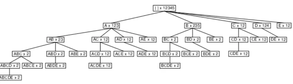
The central data structure in a vertical FI-miner is the IT-tree that represents both the search space and the final result. The IT-tree is an extended prefix-tree whose nodes are X × t(X) pairs. With respect to a classical prefix-tree or trie, in an IT-tree the itemset X provides the entire prefix from the root to the node labeled by it (and not the difference with the parent node prefix).
Example. Figure 1 presents the IT-tree of our example. Observe that the node ABC × 2 for instance can be computed by combining the nodes AB × 23 and AC ×12. To that end, tidsets are intersected and itemsets are joined. The support of ABC is readily established to 1.
3.2 Eclat
Eclat is a plain FI-miner. It traverses the IT-tree in a depth-first manner in a pre-order way, from left-to-right [18,19].
At the beginning, the IT-tree is reduced to its root (empty itemset). Eclat ex-tends the root one level downwards by adding the nodes of all frequent 1-itemsets. Then, each of the new nodes is extended similarly: first, candidate descendant nodes are formed by adding to its itemset the itemset of each right sibling; sec-ond, the tidsets are computed by intersection and the supports are established;
Fig. 1. IT-tree: Itemset-Tidset search tree of dataset D
and third, the frequent itemsets are added as effective descendant nodes of the current node.
Running example. Using Figure 1, we illustrate the execution of Eclat on dataset D with min_supp = 1 (20%). Initially, the IT-tree comprises only the root node whose support is 100%. Frequent items with their tidsets are then added under the root. Each of the new nodes is recursively extended, following a left-to-right order and processing the corresponding sub-trees in a pre-order fashion. For instance, the subtree of A comprises all frequent itemsets starting with A. Thus, at step two, all 2-long supersets of A are formed using the right siblings of A (frequent 1-itemsets). As AB, AC, AD, and AE are all frequent, they are added as descendant nodes under the node of A. The extend procedure is then recursively called on AB and the computation goes one level deeper in the IT-tree. When the algorithm stops, all frequent itemsets are discovered.
3.3 Charm
Charm adapts the computing schema of Eclat to construct FCIs only [12]. The key challenge faced by Charm is to reduce the complete IT-tree as depicted in Figure 1 to the family of FCIs. Thus, on the one hand, it has to rapidly find an FCI from a prefix thereof, i.e., without necessarily exploring all its frequent subsets. To that end, Charm applies four properties of itemset-tidset pairs (de-tailed in [12]) that help rapidly extend each itemset X to a maximal itemset Z with t(X) = t(Z) such that the former is a prefix of the latter. Yet this does not guarantee that Z is closed as γ(X) does not need to admit X as a prefix. Hence, each such Z must be checked for closeness, which calls for two enabling mecha-nisms. One is a storage of all closed itemsets allowing all candidate closures to be easily checked against the currently known ones. It is realized by means of a hash table whose hash key is based on the tidset (image) of Z (see Section 4 for further details on hashing). The second mechanism arises naturally with the traversal strategy applied in Charm: In fact, among all the candidates Z, i.e., maximally extended itemsets that share the same image, the closure γ(Z) is always generated first. Thus, to test if Z is closed, it must be checked if there is
a superset of Z with the same image already stored. If there is such a superset, then it is necessarily the closure of Z, so the current candidate is discarded.
Example. On dataset D, Charm builds a similar albeit much smaller IT-tree than the one in Figure 1. Altogether, it finds 6 closed itemsets by min_supp = 1. For instance, to determine that the itemset BD is not closed, Charm relies on the closure ABCDE. The latter is output by the processing of the branch of A, hence it is already stored when the candidate BD is created during the process of the branch of B. Thus, as BD is a subset of ABCDE with the same image, BD is discarded.
Charm is knowingly one of the fastest FCI-miners, especially for dense, highly correlated datasets. Hence our idea of using it as basis for an own FCI/FG-mining method. The challenge to face here is the proper translation of the FCI-targeting strategy in Charm to FGs. A first observation is that FGs play dual role within the corresponding equivalence classes where they are minimal, whereas FCIs are maximal. Moreover, there may be several FGs in a class, which means that the candidate check cannot rely on mere image comparison. Indeed, if two FGs happen to be checked against each other, none of them must be discarded. Thus, one needs a further test that looks for itemset inclusion: a candidate FG should be certified if there is no subset thereof with the same image stored in the FG hash. This testing principle calls for a different traversal strategy, i.e. one that insures all subsets of an itemset X are already processed before X itself. Such a requirement is typically addressed with a breadth-first, levelwise traversal strategy. Curiously enough, it can be achieved even with a depth-first one, yet not a standard one. The next section presents the traversal discipline and the algorithm built on top of it.
4
Talky-G
Talky-G is a novel vertical algorithm to find frequent generators (FGs) only. Talky-G traverses the IT-tree in a depth-first manner in a reverse pre-order way, from right-to-left.
4.1 Reverse Pre-Order Traversal
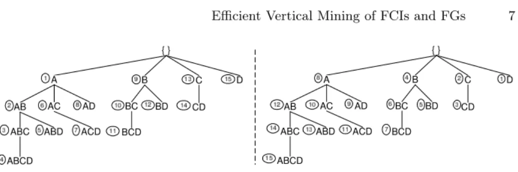
While Eclat and Charm traverse the IT-tree in a pre-order way from left-to-right, Talky-G uses the so-called reverse pre-order strategy, where the order of traversal is right-to-left. In [20], Calders and Goethals made the following observation. Let X be the itemset of a node in the IT-tree. In the case of reverse pre-order traversal, the nodes of the subsets of X are either on the path from the root node to the node of X, or are in a branch that comes in the order after X, never in a branch that comes in the order before the branch of X. That is, the same tree is processed, still in a depth-first manner, but from right-to-left. This order is called reverse pre-order. As pointed out in [20], using reverse pre-order
Fig. 2. Left: pre-order traversal with Eclat; Right: reverse pre-order traversal with Talky
traversal, all subsets of X are handled before X itself. Though no name was given in [20] to this modified version of Eclat, we will refer to this algorithm as Talky. That is, Talky is Eclat with reverse pre-order traversal. The algorithm proposed hereafter called Talky-G is a completion of this traversal in order to explore FGs only.
Example. See Figure 2 for a comparison between the two traversals namely pre-order with Eclat (left) and reverse pre-pre-order with Talky (right). The direction of traversal is indicated in circles on the left side of the nodes.
4.2 The Algorithm
Pseudo code. Algorithm 1 provides the main block of Talky-G. First, the IT-tree is initialized, which includes the following steps: the root node, representing the empty set, is created. By definition, the support of the empty set is equal to the number of transactions in the dataset (100%). Talky-G transforms the layout of the dataset in vertical format, and inserts under the root node all 1-long frequent generators.4
Then, the dataset itself can be deleted from the main memory since all frequent generators are unions of 1-long frequent generators. After this, the extend procedure is called recursively for each child of the root in a reverse pre-order way from right-to-left. Talky-G concentrates on frequent generators only so that at the end all FGs are comprised in the IT-tree.
The addChild procedure inserts an IT-node under a node. The save proce-dure stores a frequent generator in a dedicated “list” data structure.
The extend procedure (see Algorithm 2) discovers all frequent generators in the subtree of a node. First, the procedure forms new frequent generators with the right siblings of the current node. Then, these FGs are added below the current node and are extended recursively in a reverse pre-order way from right-to-left.
The getNextGenerator function (see Algorithm 3) has two nodes as input parameters, and it returns a new frequent generator, or “null” if no frequent
4
Fig. 3. Execution of Talky-G on dataset D with min_supp = 1 (20%)
generator can be produced from the two input nodes. A candidate node is created by taking the union of the itemsets of the two input nodes, and the intersection of their tidsets. Thus, the input nodes are the parents of the candidate. Then, the candidate undergoes a series of tests. First, a frequency test is used to eliminate non-frequent itemsets. Second, the candidate is compared to its parents. If its tidset is equivalent to the tidset of one of its parents, then the candidate is not generator by Def. 1. If an itemset passed these two tests, it is still not sure that it is generator. As seen before, the reverse pre-order traversal guarantees that when an itemset is reached in the IT-tree, all its subsets are handled before. Talky-G collects frequent generators in a “list” too (see also the save procedure). The third test checks if the candidate has a proper subset with the same support in this “list”. If yes, then the candidate is not generator by Def. 1. This last step might seem to be a very expensive step, but as we will see later, it can be done very efficiently with a special hash data structure. If a candidate survives all the tests, then it is an FG and will be added to the IT-tree. Otherwise it is discarded and this prevents any of its supersets to be generated as candidates (see Prop. 1). This way, the search space is reduced to frequent generators only.
When the algorithm stops, all frequent generators (and only frequent generators) are inserted in the IT-tree and in the “list” of generators.
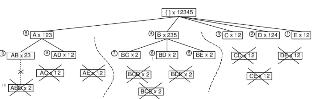
Running example. The execution of Talky-G on dataset D with min_supp = 1 (20%) is illustrated in Figure 3. The execution order is indicated on the left side of the nodes in circles.
The algorithm first initializes the IT-tree with the root node. Since there is no full column in the input dataset, all attributes are frequent generators, thus they are added under the root. The children of the root node are extended recursively one by one, from right-to-left. Node E has no right sibling, thus it cannot be extended. Node D is extended with E, but the resulting itemset DE is not generator since its support is equal to the support of its parent E. Node C is extended with D and E, but neither CD nor CE is generator for the same reason. We skip the detailed presentation of the subtree of B. 2-long supersets of A are formed by using its right siblings and added to the IT-tree. The candidates AC
Algorithm 1 (main block of Talky-G):
1) root.itemset ← ∅; // root is an IT-node whose itemset is empty
2) root.tidset ← {all transaction IDs}; // the empty set is included in every tr.
3) loop over the vertical representation of the dataset (attr) { 4) if ((attr.supp ≥ min_supp) and (attr.supp < |O|)) { 5) root.addChild(attr); // attr is frequent and generator
6) } 7) } 8)
9) loop over the children of root from right-to-left (child) { 10) save(child); // process the itemset
11) extend(child); // discover the subtree below child
12) }
Algorithm 2 (“extend” procedure of Talky-G):
Method: extend an IT-node recursively (discover FGs in its subtree) Input: curr – an IT-node whose subtree is to be discovered
1) loop over the siblings of curr from left-to-right (other) { 2) generator ← getNextGenerator(curr, other);
3) if (generator 6= null) then curr.addChild(generator); 4) }
5)
6) loop over the children of curr from right-to-left (child) { 7) save(child); // process the itemset
8) extend(child); // discover the subtree below child
9) }
and AE are not generators because of C and E, respectively. The combination of AB and AD produces the candidate ABD, which represents a special case. Its support is different from its parents, but we already found a proper subset of it with the same support (BD) in a previous branch. According to Def. 1, ABD is not generator, thus it is not added to the IT-tree.
4.3 Fast Subsumption Checking
Let Xiand Xjbe two itemsets. We say that Xisubsumes Xj (or Xj is subsumed
by Xi), iff Xj ⊂ Xi and supp(Xi) = supp(Xj). Xi (resp. Xj) is also known as
subsumer (resp. subsumee). By Def. 1, if an itemset subsumes another itemset, then the subsumer is not generator. Recall that in the getNextGenerator func-tion, when a new candidate itemset C is created, Talky-G checks if C subsumes a previously found generator. If the test is positive, then clearly C is not
gener-Algorithm 3 (“getNextGenerator” function of Talky-G):
Method: create a new frequent generator Input: two IT-nodes (curr and other) Output: a frequent generator or null
1) cand.tidset ← curr.tidset ∩ other.tidset;
2) if (cardinality(cand.tidset) < min_supp) { // test 1
3) return null; // not frequent
4) }
5)// else, if it is frequent
6) if ((cand.tidset = curr.tidset) or (cand.tidset = other.tidset)) { // test 2
7) return null; // not generator
8) }
9)// else, if it is a potential generator
10) cand.itemset ← curr.itemset ∪ other.itemset;
11) if (cand has a proper subset with the same support in the hash) { // test 3
12) return null; // not generator
13) }
14)// if cand passed all the tests then cand is a frequent generator
15) return cand;
ator. This subsumption test might seem to be an expensive step, but we found a very efficient way to filter these non-generator itemsets.
In Talky-G we adapted the hash structure of Charm for storing frequent generators. Talky-G, similarly to Charm, computes a hash function on the sum of the tids in the tidset and stores in the hash table a generator with its support value. Due to the tidset-based hash function, two itemsets with the same image have the same hash value. Itemsets having the same hash value are stored in a list at the same position of the hash. Let h(Xi) denote the hash function on the
tidset of Xi. For the subsumption check of a candidate itemset C, we retrieve
from the hash table all entries with the hash key h(C). For each element G in this list, test if supp(C) = supp(G). If yes, test if C ⊃ G. If yes, then C subsumes G, i.e. C is not generator. If C subsumes no entries in the list, then C is generator and added to the end of the list.
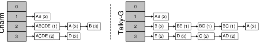
Example. Let us see Figure 4 (right) that depicts the hash structure of the IT-tree in Figure 3. This hash table contains all frequent generators of dataset D. For this example, the size of the hash table is set to four.5
At each position of the hash table there are pointers to lists. In each list we can find itemsets that have the same hash key.
In the running example we saw that ABD is not generator. It can be deter-mined the following way. First, compute the sum of the tids in its tidset; then
5
Fig. 4. Hash tables for dataset D by min_supp = 1. Left: hash table of Charm containing all FCIs; Right: hash table of Talky-G containing all FGs
modulo this sum by the size of the hash table to get its hash value: 2 mod 4 = 2. Traverse the list of the hash table at position 2. The support of B differs from the support of ABD. The itemset BE has the same support value as ABD, but ABD is not a proper superset of BE. The itemset BD has the same support as ABD, and ABD is a proper superset of BD, thus ABD is not generator. At this point the traversal of the list is finished.
Experimental results of Talky-G are reported in the next section as part of the Touch algorithm.
5
Touch
The Touch algorithm has three main features, namely (1) extracting frequent closed itemsets, (2) extracting frequent generators, and (3) associating frequent generators to their closures, i.e. identifying frequent equivalence classes.
5.1 The Algorithm
Previously, we showed that Charm and Talky-G extract frequent closed itemsets and frequent generators, respectively. Each algorithm uses a dedicated hash data structure for storing the found itemsets (see Figure 4). There is one more step to do namely associating frequent generators to their closures, i.e. identifying the equivalence classes. The question is how to do this efficiently.
Our approach uses the hash structures for the association. The method is based on the following property:
Property 2. Let h(X) denote the hash function on the tidset of X. Given a frequent closed itemset Y and its frequent generator Z, h(Y ) = h(Z) since t(Y ) = t(Z).
Since the two hash tables have the same size, and the two algorithms use the same hash function, it follows from Property 2 that a frequent closed itemset and its generators are in different hash tables but at the same index position.
Pseudo code. The pseudo code of Touch is given in Algorithm 4. First, the algorithm calls Charm and Talky-G and takes over their hash structures. Then,
Algorithm 4 (Touch):
Description: find frequent equivalence classes
1) hashF CI ←(call Charm and get its hash data structure); // see Section 3.3
2) hashF G ←(call Talky-G and get its hash data structure); // see Section 4
3) match(hashF CI, hashF G);
Table 1. Output of Touch on dataset D by min_supp = 1
FCI (supp) FGs AB (2) AB ABCDE (1) BE; BD; BC A (3) A FCI (supp) FGs B (3) B ACDE (2) E; C; AD D (3) D
Touch matches the two hash tables the following way. For each frequent closed itemset X, it looks up in the other hash table at the same index position all subsets of X that have the same support. The output of Touch is shown in Table 1. Recall that due to the property of equivalence classes, the support of a generator is equal to the support of its closure.
Example. Consider Figure 4 that depicts the hash structures of Charm and Talky-G. Say we want to determine the generators of the closed itemset ACDE. The itemset ACDE is stored at position 3 in the hash structure of Charm. By Property 2, its generators are also stored at position 3 in the hash structure of Talky-G. In this list, there are three itemsets that are subsets of ACDE and that have the same support values: E, C, and AD. It means that these three itemsets are the generators of ACDE. The frequent closed itemset A has one subset with the same support in the other hash structure at index 2 (A). This means that A is a closed itemset and a generator at the same time, i.e. the equivalence class of A has one element only (singleton equivalence class). Etc.
5.2 Experimental Results
We evaluated Touch against Zart [11] and A-Close [8]. The algorithms were implemented in Java in the Coron data mining platform [21].6
The experiments were carried out on a bi-processor Intel Quad Core Xeon 2.33 GHz machine running under Ubuntu GNU/Linux operating system with 4 GB of RAM. For the experiments we have used the following datasets: T20I6D100K, C20D10K, and Mushrooms. The T20I6D100K7
is a sparse dataset, constructed according to the properties of market basket data that are typical weakly correlated data.
6
http://coron.loria.fr
7
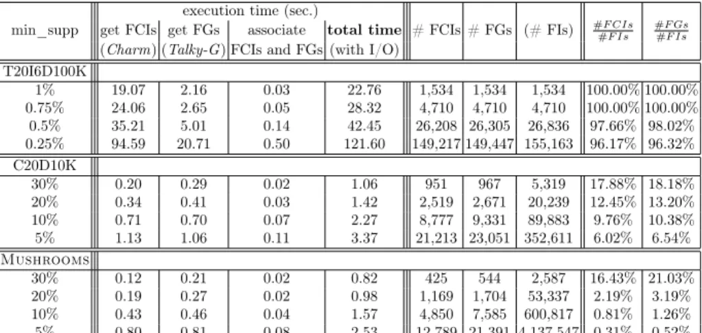
Table 2. Detailed execution times of Touch and other statistics (number of FCIs, number of FGs, number of FIs, proportion of the number of FCIs to the number of FIs, proportion of the number of FGs to the number of FIs). Note that the number of FIs is shown for comparative reasons only. Touch does not need to extract all FIs
execution time (sec.)
min_supp get FCIs get FGs associate total time # FCIs # FGs (# FIs) #F CIs #F Is
#F Gs #F Is
(Charm) (Talky-G) FCIs and FGs (with I/O) T20I6D100K 1% 19.07 2.16 0.03 22.76 1,534 1,534 1,534 100.00% 100.00% 0.75% 24.06 2.65 0.05 28.32 4,710 4,710 4,710 100.00% 100.00% 0.5% 35.21 5.01 0.14 42.45 26,208 26,305 26,836 97.66% 98.02% 0.25% 94.59 20.71 0.50 121.60 149,217 149,447 155,163 96.17% 96.32% C20D10K 30% 0.20 0.29 0.02 1.06 951 967 5,319 17.88% 18.18% 20% 0.34 0.41 0.03 1.42 2,519 2,671 20,239 12.45% 13.20% 10% 0.71 0.70 0.07 2.27 8,777 9,331 89,883 9.76% 10.38% 5% 1.13 1.06 0.11 3.37 21,213 23,051 352,611 6.02% 6.54% Mushrooms 30% 0.12 0.21 0.02 0.82 425 544 2,587 16.43% 21.03% 20% 0.19 0.27 0.02 0.98 1,169 1,704 53,337 2.19% 3.19% 10% 0.43 0.46 0.04 1.57 4,850 7,585 600,817 0.81% 1.26% 5% 0.80 0.81 0.08 2.53 12,789 21,391 4,137,547 0.31% 0.52%
The C20D10K is a census dataset from the PUMS sample file, while the Mush-rooms8
describes mushrooms characteristics. The last two are highly correlated datasets.
Table 2 contains detailed information about the execution of Touch. The first three columns correspond to the three main steps of Touch namely (1) getting FCIs using Charm, (2) getting FGs using Talky-G, and (3) associating FGs to their closures. Column 4 indicates the total execution time of the algorithm including input and output. In the sparse dataset T20I6D100K, almost all fre-quent itemsets are closed and generators at the same time. It means that most equivalence classes are singletons. It is known that Charm is less efficient on sparse datasets. This is due to the fact that Charm performs four tests on can-didates for reducing the IT-tree. However, in sparse datasets the number of FCIs is almost equivalent to the number of FIs, thus the search space cannot be re-duced significantly. Talky-G is also less efficient on sparse datasets. However, in dense, highly correlated datasets (C20D10K and Mushrooms), both Charm and Talky-G are very efficient, even at low minimum support values. Since the number of FCIs and FGs is much less than the number of FIs, the two algorithms can take advantage of exploring a much smaller search space. The association of FCIs and FGs is done very efficiently in all cases. That is, the association step gives absolutely no overhead to Touch.
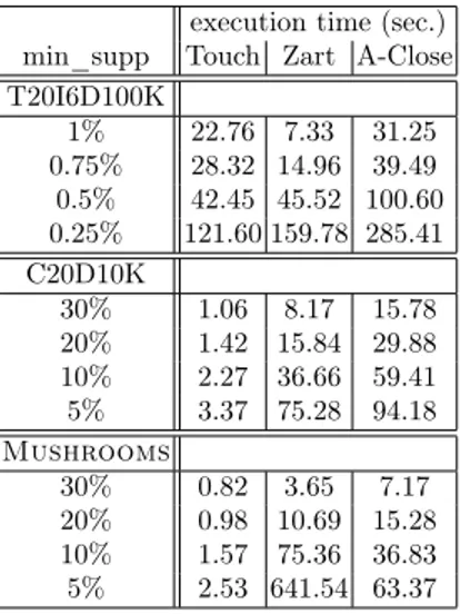
Table 3 contains the experimental evaluation of Touch against Zart and A-Close. All times reported are real, wall clock times as obtained from the Unix
8
Table 3. Response times of Touch, compared to Zart and A-Close
execution time (sec.) min_supp Touch Zart A-Close T20I6D100K 1% 22.76 7.33 31.25 0.75% 28.32 14.96 39.49 0.5% 42.45 45.52 100.60 0.25% 121.60 159.78 285.41 C20D10K 30% 1.06 8.17 15.78 20% 1.42 15.84 29.88 10% 2.27 36.66 59.41 5% 3.37 75.28 94.18 Mushrooms 30% 0.82 3.65 7.17 20% 0.98 10.69 15.28 10% 1.57 75.36 36.83 5% 2.53 641.54 63.37
time command between input and output. We have chosen Zart and A-Close because they represent two efficient algorithms that produce exactly the same output as Touch. Zart and A-Close are both levelwise algorithms. Zart is an extension of Pascal [14], i.e. first it finds all FIs using pattern-counting inference, then it filters FCIs, and finally the algorithm associates FGs to their closures. A-Close reduces the search space to FGs only, then it calculates the closure for each generator. The way A-Close computes the closures of generators is quite expensive because of the huge number of intersection operations. Touch, just like A-Close, reduces the search space to the strict minimum, i.e. it only extracts what it really needs namely the set of FCIs and the set of FGs. Then, Touch associates the two sets in a very efficient way. Since Touch is based on Charm and Talky-G, the algorithm is very efficient on dense, highly correlated datasets. We must admit however that levelwise algorithms like Zart are sometimes more suitable for sparse datasets.
6
Conclusion
Mining FGs has so far been done largely in a levelwise manner as the breadth-first traversal fits the down-set structure of the FG family. Yet depth-first algorithms have shown superior efficiency in many situations, whence the motivation of our study of depth-first FCI/FG-mining.
As a contribution to this problem, we presented Touch, an algorithm that splits the general problem into three tasks: (1) FCI-mining, (2) FG-mining, and (3) association of FGs to their closures (FCIs). While (1) is solved by reusing an existing algorithm, Charm, the two others generate innovative solutions. Hence the Talky-G vertical FG-miner used in (2) is an original contribution on its own. As all three solutions are highly optimized, the algorithm performs well
against comparable levelwise miners. Numerous concise representations of valid association rules can be readily derived from the method output.
The study led to a range of exciting questions that are currently investigated. Thus, from an algorithmic point of view, it would be interesting to merge steps (1) and (2), e.g. by using the output of Talky-G (i.e., the IT-tree of all FGs) as a starting point for the FCI-mining, hence avoiding step (3). A further challenge lays in the computation of the FCI precedence order that underlies some of the association rule bases from the literature.
References
1. Agrawal, R., Srikant, R.: Fast Algorithms for Mining Association Rules in Large Databases. In: Proc. of the 20th Intl. Conf. on Very Large Data Bases (VLDB ’94), San Francisco, CA, USA, Morgan Kaufmann Publishers Inc. (1994) 487–499 2. Bastide, Y., Taouil, R., Pasquier, N., Stumme, G., Lakhal, L.: Mining Minimal Non-Redundant Association Rules Using Frequent Closed Itemsets. In: Proc. of the Computational Logic (CL ’00). Volume 1861 of LNAI., Springer (2000) 972–986 3. Kryszkiewicz, M.: Representative Association Rules. In: Proc. of the 2nd
Pacific-Asia Conf. on Research and Development in Knowledge Discovery and Data Mining (PAKDD ’98), Melbourne, Australia, Springer-Verlag (1998) 198–209
4. Pasquier, N., Bastide, Y., Taouil, R., Lakhal, L.: Closed set based discovery of small covers for association rules. In: Proc. 15emes Journees Bases de Donnees Avancees (BDA). (1999) 361–381
5. Duquenne, V.: Contextual implications between attributes and some representa-tional properties for finite lattices. In: Beitraege zur Begriffsanalyse, B.I. Wis-senschaftsverlag, Mannheim (1987) 213–239
6. Luxenburger, M.: Implications partielles dans un contexte. Mathématiques, Infor-matique et Sciences Humaines 113 (1991) 35–55
7. Kryszkiewicz, M.: Concise Representations of Association Rules. In: Proc. of the ESF Exploratory Workshop on Pattern Detection and Discovery. (2002) 92–109 8. Pasquier, N., Bastide, Y., Taouil, R., Lakhal, L.: Discovering frequent closed
item-sets for association rules. In: Proc. of The 7th Intl. Conf. on Database Theory (ICDT ’99), Jerusalem, Israel (1999) 398–416
9. Stumme, G., Taouil, R., Bastide, Y., Pasquier, N., Lakhal, L.: Computing Iceberg Concept Lattices with TITANIC. Data and Knowledge Engineering 42(2) (2002) 189–222
10. Valtchev, P., Missaoui, R., Godin, R.: Formal Concept Analysis for Knowledge Discovery and Data Mining: The New Challenges. In: Proc. of the 2nd Intl. Conf. on Formal Concept Analysis, Springer Verlag (Feb 2004) 352–371
11. Szathmary, L., Napoli, A., Kuznetsov, S.O.: ZART: A Multifunctional Itemset Mining Algorithm. In: Proc. of the 5th Intl. Conf. on Concept Lattices and Their Applications (CLA ’07), Montpellier, France (Oct 2007) 26–37
12. Zaki, M.J., Hsiao, C.J.: CHARM: An Efficient Algorithm for Closed Itemset Min-ing. In: SIAM Intl. Conf. on Data Mining (SDM’ 02). (Apr 2002) 33–43
13. Pei, J., Han, J., Mao, R.: CLOSET: An Efficient Algorithm for Mining Frequent Closed Itemsets. In: ACM SIGMOD Workshop on Research Issues in Data Mining and Knowledge Discovery. (2000) 21–30
14. Bastide, Y., Taouil, R., Pasquier, N., Stumme, G., Lakhal, L.: Mining frequent patterns with counting inference. SIGKDD Explor. Newsl. 2(2) (2000) 66–75
15. Boulicaut, J.F., Bykowski, A., Rigotti, C.: Free-Sets: A Condensed Representation of Boolean Data for the Approximation of Frequency Queries. Data Mining and Knowledge Discovery 7(1) (Jan 2003) 5–22
16. Kryszkiewicz, M.: Concise Representation of Frequent Patterns Based on Disjunction-Free Generators. In: Proc. of the 2001 IEEE Intl. Conf. on Data Mining (ICDM ’01), Washington, DC, USA, IEEE Computer Society (2001) 305–312 17. Ganter, B., Wille, R.: Formal concept analysis: mathematical foundations.
Springer, Berlin/Heidelberg (1999)
18. Zaki, M.J., Parthasarathy, S., Ogihara, M., Li, W.: New Algorithms for Fast Discovery of Association Rules. In: Proc. of the 3rd Intl. Conf. on Knowledge Discovery in Databases. (August 1997) 283–286
19. Zaki, M.J.: Scalable Algorithms for Association Mining. IEEE Transactions on Knowledge and Data Engineering 12(3) (2000) 372–390
20. Calders, T., Goethals, B.: Depth-first non-derivable itemset mining. In: Proc. of the SIAM Intl. Conf. on Data Mining (SDM ’05), Newport Beach, USA. (Apr 2005)
21. Szathmary, L.: Symbolic Data Mining Methods with the Coron Platform. PhD Thesis in Computer Science, Univ. Henri Poincaré – Nancy 1, France (Nov 2006)