HAL Id: hal-00000692
https://hal.archives-ouvertes.fr/hal-00000692
Preprint submitted on 8 Oct 2003
HAL is a multi-disciplinary open access
archive for the deposit and dissemination of sci-entific research documents, whether they are pub-lished or not. The documents may come from teaching and research institutions in France or
L’archive ouverte pluridisciplinaire HAL, est destinée au dépôt et à la diffusion de documents scientifiques de niveau recherche, publiés ou non, émanant des établissements d’enseignement et de recherche français ou étrangers, des laboratoires
On certain perturbations of the Erdös-Renyi random
graph
Stéphane Coulomb, Michel Bauer
To cite this version:
Stéphane Coulomb, Michel Bauer. On certain perturbations of the Erdös-Renyi random graph. 2003. �hal-00000692�
ccsd-00000692 (version 1) : 8 Oct 2003
On certain perturbations of the
Erd¨
os-Renyi random graph
St´ephane Coulomb
1and Michel Bauer
2Service de Physique Th´eorique de Saclay
3CE Saclay, 91191 Gif sur Yvette, France
Abstract
We study perturbations of the Erd¨os-Renyi model for which the statistical weight of a graph depends on the abundance of certain geometrical patterns. Using the formal correspondance with an ex-actly solvable effective model, we show the existence of a percolation transition in the thermodynamical limit and derive perturbatively the expression of the threshold. The free energy and the moments of the degree distribution are also computed perturbatively in that limit and the percolation criterion is compared with the Molloy-Reed criterion.
1
Introduction
Random graphs were introduced more than forty years ago by mathemati-cians and have proved since then to be a very useful and versatile concept. The most studied example is the Erd¨os-Renyi model [5], where the edges are independent. Balanced with the simplicity of its definition, the richness and deepness of mathematical results are really fascinating.
On the other hand, it is clear that the Erd¨os-Renyi model is a poor idealization of real networks, those which pop out naturally in sociology, biology, communication sciences,... For instance, the degree distribution (i.e. the statistics of the number of edges incident at a vertex) of most of the real life examples exhibits statistical, scale-free, properties very far from the poissonian behavior predicted by the Erd¨os-Renyi model [1],[4].
1
Email: [email protected]
2
Email: [email protected]
3
Laboratoire de la Direction des Sciences de la Mati`ere du Commisariat `a l’Energie Atomique, URA2306 du CNRS
Many random graph models are now on the market, some consructed ad hoc to reproduce certain desired features needed to fit real data, some con-structed according to general principles. Belonging to the second category, the Molloy-Reed model [6] concentrates, inside the space of all labeled graphs with uniform probability, on the subspace of graphs with an arbitrarily given degree distribution. Within this model, many relevant quantities can be com-puted analytically, and there is a general percolation criterion given in terms of cumulants of the edge degree distribution.
Our aim is to study another family of random graphs for which explicit computations are also possible. The idea is roughly as follows. Suppose that to each graph G one assigns a weight u(G). From the weight u one can construct another weight w(G) = P
G′⊂Gu(G) where the sum is over graphs G′ with the same vertex set as G and edge set included in that of
G. Conversely, from any weight function w one can extract a unique weight function u, but the expression of u in terms of w involves minus signs.
We shall introduce a model for which the weight u is a counting function for certain structures on graphs. This weight u has two further properties : first it is permutation invariant, i.e. the weight of a graph does not depend on the labelling of its vertices, and second it factors over connected components, i.e the weight for a graph with several connected components is the prod-uct of the weight of each component. Note that by standard combinatorial arguments, these three properties are inherited by the weight w.
Then we study the thermodynamic finite connectivity limit, when the size of the system (i.e. the number of vertices of the graph) becomes large but the average number of neighbors of any given vertex has a fixed finite value. In this regime, the relevant features of the weights u and w are encoded in tree generating functions u and w respectively.
The idea is that because u counts less objects than w (which is not true for arbitrary w because then u does not have a simple combinatorial in-terpretation in general), the generating function u has better convergence properties than the corresponding generating function w. We shall make the (crucial) assumption that the first singularity in the generating function of w can be obtained from the functional relation that ties it to the generat-ing function of u, without havgenerat-ing to know the sgenerat-ingularities of the generatgenerat-ing function for u itself. This is certainly true, as we shall recall later, for the Erd¨os-Renyi model. It is also true order by order in perturbation theory around the Erd¨os-Renyi model for the models we introduce. We shall have little to say analytically on non perturbative properties, but the numerical simulations are encouraging.
Under this assumption we are able to give expressions for the free energy, the size distribution of connected components and for the percolation
cri-terion and size of the giant component when it exists. The expressions are not very explicit, because they involve the function u, which is very compli-cated in terms of the original parameters of the model. So on the one hand we show how to perform explicit perturbative computations of the physical quantities and on the other hand we introduce an effective model for which the relationship between u and u is directly computable,
Our motivations are the following. First the models we study form a natu-ral and reasonnably manageable family of random graph models. Our point is to emphasize the connection with quantum field theory. We do not claim that the relation is very deep, but many random graph phenomena have quantum field theory counterparts, and quantum field theory gives a very convenient language and insight. Second, one of the interests of studying models with non trivial degree correlations is that attacks (see e.g. [7],[8]) automatically induce such features, even if they were absent to begin with. Third, at a more basic level, we can contrast with the Molloy-Reed model. This is use-ful for the purpose of general comparison, but especially because heuristic arguments, always based on non explicit assumptions, allow to recover the Molloy-Reed percolation criterion whitout using the particular hypothesis of the Molloy-Reed model, thereby suggesting that the Molloy-Reed percolation criterion has a much wider range of validity. This is probably wrong, and the model solved in this paper is definitely not in this range.
2
The model
After recalling the elementary graph theoretic definitions, we present our basic assumptions. We use the framework of statistical mechanics, i.e. we assign to each labelled graph of size N a weight (real positive number), which we use as an unnormalized probability distribution. For the Erd¨os-Renyi model, the weight is simply pE(G)(1− p)N (N −1)2 −E(G) where E(G) is the
number of edges of G. We shall choose a weight function that depends on more detailed local features of the graph, namely the abundance of certain geometric motives.
2.1
A few definitions and notations
Simple unoriented graphs, connected graphs, trees. A (simple un-oriented) graph G is a couple (V, E) where V 6= ∅ is the vertex set and E ⊂ {{i, j}; i, j ∈ V, i 6= j} is the edge set. If V = {1, ⋅ ⋅ ⋅ , N} for some integer N , then G is called a labelled graph. The set of labelled graphs of size N is denoted GN.
If G is a graph, we denote by V (G) the vertex set of G or the cardinal of this vertex set, depending on the context, i.e whether a set or a number is expected at that place 1. Similarly, E(G) will denote either the edge set of
G or the cardinal of this edge set.
A connected component of G is a minimal graph (V′, E′) with V′ ⊂ V such
that if (i, j)∈ V′· V and {i, j} ∈ E then j ∈ V′ and {i, j} ∈ E′.
A connected graph is a graph which has only one connected component. A circuit of G of size s is a sequence (i1,⋅ ⋅ ⋅ , is) of distinct vertices with s≥ 3
such that {i1, i2}, ⋅ ⋅ ⋅ , {is−1, is} and {is, i1} are edges.
A tree is a connected graph without circuits, and the set of labelled trees of size N is denoted by TN.
If {i, j} is an edge of G, we say that i and j ∈ V are neighbours in G. The number of neighbours of a given vertex i ∈ V in a graph G, also called the degree of G at vertex i, is denoted li(G), or li when there is no ambiguity. It
is the number of elements of E in which i appears.
Adjacency matrix of a graph, operations on matrices. The adja-cency matrix A(G) (or simply A) of a labelled graph G ∈ GN is the N by
N matrix defined by Ai,j = 1 if {i, j} is an edge of G, Ai,j = 0 else. Note
that the set of adjacency matrices is the set of symmetric 0, 1 matrices with vanishing diagonal elements.
The sum of all elements of any matrix M will be written kMk ≡ P
i,jMi,j.
If M is the adjacency matrix A(G) of a graph G, then it is clear that 1 2kMk
is E(G), the number of edges of G.
The sum of all diagonal elements of a square matrix M is the trace of M , written T r(M ). Note that 1
2T r(A(G)
2) is again equal to E(G).
2.2
Probability distribution, partition function
To emphasize the similarities between the random graph model studied in this paper and quantum field theory, we split the weight of graphs in a product of a free part and an interacting part. The free weight is w0(G)≡ qE(G) where
q ∈]0, +∞[. For later convenience, we also introduce p = q/(1 + q) ∈]0, 1[. The interacting part is wI(G)≡ eSI(G), where
SI(G)≡ X k tk 2kT rA(G) k+X k sk 2kA(G) k k. 1
This should cause no confusion, though from a fundamental point of view, a number is a set as well.
The full weight is w(G) ≡ w0(G)wI(G). The normalization factor included
in the definition of the partition function ZN ≡ (1 − p) N (N −1) 2 X G∈GN w(G)
is chosen in such a way that ZN can be expressed as an average over
Erd¨os-Renyi weights :
ZN =eSI(G)
®
ER(p),
where ER(p) assigns probability pE(1−p)N (N −1)2 −E to any graph on N vertices
with E edges. We view w0 as describing a gas of independent edges (the
Erd¨os-Renyi model), and SI as describing the interactions between edges,
the tk’s and sk’s being arbitrary real parameters that regulate the abundance
of certain local geometric features of G. Note that if G is made of several connected components, G1,⋅ ⋅ ⋅ , Gl, SI(G) = SI(G1) +⋅ ⋅ ⋅ + SI(Gl), so that
wI factors as a product over connected components. This is also true of
w0. This multiplicativity of the weight plays a crucial role to simplify the
analysis below. Another striking feature is that w(G) is invariant under permutations of the vertex set. Many other interactions with this property could be incorporated, for instance by including products of traces and norms into the interaction, however these would break the multiplicativity property. The “simple” multiplicative model does not seem to be exactly solvable, and we have to rely on perturbation theory to make explicit computations. Even the “trival” case when all parameters except, say, s3 vanish is already
complicated enough. This is why we insist on keeping the two properties : multiplicativity and permutation invariance.
The above model is perfectly well defined for all parameter values as long as N is finite. However, we shall be interested in taking a large N limit such that the average degree is a fixed number (so that the number of edges is proportional to N ). This will impose some constraints, see below.
3
Two combinatorial formulæ for the
parti-tion funcparti-tion
In this section, we shall derive two formulæ related to exponentiation in combinatorics.
3.1
Connected components
Suppose we consider the grand canonical partition function
Ξ =X
G
w(G) V (G)!z
V (G)
as a power series in z : this is a formal sum over all graphs of any size, from which ZN can be recovered as
ZN = (1− p) N (N −1) 2 N ! I dz zN +1Ξ(z)
where for the time being, the symbol H dz
zN +1 is not viewed as a real contour integral, but simply as the operation of taking the term of order N in the z expansion of a formal power series. If G has l connected components G1,⋅ ⋅ ⋅ , Gl, we observe that w(G) V (G)!z V (G) = 1 ³ Pl k=1V (Gk) ´ ! l Y k=1 qE(Gk)w I(Gk)zV (Gk).
Summing over G is the same as summing over the connected components. Up to now the vertices of the Gk were labelled as subgraphs of G. Thanks to
permutation invariance, one can instead sum over abstract finite sequences of l = 1, 2,⋅ ⋅ ⋅ labelled connected graphs but weight the terms in the sum by a combinatorial factor 1 l! ³ Pl k=1V (Gk) ´ ! Q kV (Gk)!
to take into account all possibilities to order them and to label the union of their vertex sets from 1 to P
kV (Gk). Then Ξ = eW where W = Pc G w(G) V (G)!z V (G) ≡ P n Wn n! z
n is defined exactly as Ξ except that the sum is
only over connected graphs (this is what is meant by the symbol Pc
G). The
main formula of this section, the first exponential formula, relates ZN and
W (z) as ZN = (1− p) N (N −1) 2 N ! I dz zN +1e W (z). (1)
3.2
Reorganization of the perturbative expansion
The case when tk = sk = 0 for all k corresponds to the Erd¨os-Renyi model.
The probability of a graph only depends on the number of its edges, and many quantities such as degree distributions, component distributions and
percolation threshold take a simple form. When one or more of the tk’s and
sk’s are not vanishing, the finer structure of the graph becomes relevant, and
this will be the case of interest in this paper.
Let us fix G and start from the expansion of eSI(G) in powers of t
k’s and
sk’s. This gives a linear combination of terms of the form:
Y
k
¡¡T rA(G)k¢mk
kA(G)kknk¢ .
If we expand each matrix product, such a term becomes a sum of products of matrix elements of A(G) of generic form A(G)i1j1A(G)i2j2⋅ ⋅ ⋅ A(G)injn and we may assume that i1 6= j1,⋅ ⋅ ⋅ , in 6= jn because otherwise the product
is 0 for any (simple graph) adjacency matrix. On the other hand, to any sequence i1j1⋅ ⋅ ⋅ injn with i1 6= j1,⋅ ⋅ ⋅ , in 6= jn, we may associate a graph
H with vertex set [1, N ] and edge set {{i1, j1}, ⋅ ⋅ ⋅ , {in, jn}}. The product
A(G)i1j1A(G)i2j2⋅ ⋅ ⋅ A(G)injn vanishes unless all edges of H are edges of G, in which case it has value 1.
With this observation in mind, we define eSI(G) by keeping, in the ex-pansion of eSI(G), only those terms A(G)
i1j1A(G)i2j2⋅ ⋅ ⋅ A(G)injn such that {{i1, j1}, ⋅ ⋅ ⋅ , {in, jn}} exhausts the edge set of G (maybe with repetitions).
Then by definition,
eSI(G) = X
H,E(H)⊂E(G)
eSI(H),
where the sum is over all graphs on the same vertex set as G whose edge set is a subset of that of G. The reciprocal formula is given by eSI(H) = P
G,E(G)⊂E(H)(−)E(H)−E(G)eSI(G)and the multiplicative property of eSI(G)
en-sures that eSI(H) is also multiplicative : if H has l connected components H1,⋅ ⋅ ⋅ , Hl, eSI(H) = eSI(H1)⋅ ⋅ ⋅ eSI(Hl). Now ZN = X G∈GN (1− p)N (N −1)2 −E(G)pE(G)eSI(G) = X G∈GN X H,E(H)⊂E(G) (1− p)N (N −1)2 −E(G)pE(G)eSI(H) = X H∈GN X G,E(G)⊃E(H) (1− p)N (N −1)2 −E(G)pE(G)eSI(H). For fixed H, P G,E(G)⊃E(H)(1− p) N (N −1)
2 −E(G)pE(G) = pE(H), and we find that ZN =
X
H∈GN
Defining u(H) = pE(H)eSI(H) U = Pc H u(H) V (H)!z V (H) ≡P nUn!nz n,
we can repeat the steps leading from multiplicativity and permutation in-variance to eq.(1) to obtain the second exponential formula
ZN = N !
I dz zN +1e
U (z). (2)
3.3
Consequences of the exponential formulæ
The two expressions obtained for the partition function, one in terms of W (z) and the other in terms of U (z), show that for every nonnegative integer N
(1− p)−N (N −1)2 I dz zN +1e U (z) = I dz zN +1e W (z).
It is convenient to eliminate N by the following trick : putting 1−p = e−˻,
(1− p)−N (N −1)2 takes the form of a gaussian integral √1
2̉˻ R+∞ −∞ e− y2 2˻+yN −˻ N 2.
From the change of variable x = zey−˻2, it follows that
eW (z) = √1 2πβ Z +∞ −∞ e−y22˻+U (ze y−˻2) dy. (3)
There is no good reason why e−y22˻+U (zey− ˻
2)
should be integrable in y along the full real axis. However, if one expands this function in powers of z, term by term integration is ok, and for the time being, eq.(3) is a shorthand notation for the fact that this term by term integration leads to the formal power series of eW (z).
4
Practical perturbative expansion
Our aim is to organize the perturbative expansion to make explicit compu-tations. We would like to make a systematic enumeration of the terms that appear in perturbation theory.
A typical term in the perturbative expansion is of the form Ai1j1⋅ ⋅ ⋅ Ainjn to which we associate the sequence i1j1⋅ ⋅ ⋅ injn i.e. a word written using
the alphabet [1, N ]. For a graph G with adjacency matrix Aij, the product
Ai1j1Ai2j2⋅ ⋅ ⋅ Ainjn is 1 if{i1, j1}, ⋅ ⋅ ⋅ , {in, jn} are amongst the edges of G and 0 else. If l is the number of distinct edges among these n 2-sets, the average
is simply the sum of the Erd¨os-Renyi weights of all graphs containing these l edges. This is known to yield hAi1j1Ai2j2⋅ ⋅ ⋅ AinjniER(p) = p
l. This average
is invariant under permutations of [1, N ], all vertices play the same role in T rA(G)k andkA(G)kk. So we regroup the words i
1j1⋅ ⋅ ⋅ injnin classes under
the action of the permutation group, compute the size of each class and find a representative in each class. Then we enumerate the representatives and take multiplicities into account.
The idea is the following : suppose that you have a finite word written using any alphabet (i.e. any set of symbols) on, say, N letters. To each letter that appears in the word, associate an integer as follows : assign 1 to the first letter of the word, then assign 2 to the next new (i.e distinct from the first) letter appearing in the word, then 3 to the next new (i.e distinct from the first and the second) and so on until all letters appearing in the word have been assigned a number, the highest one being, say, v (v is the number of distinct letters used to compose the word, which may well be strictly smaller than the length of the word, because the same letter can appear more than once). Replacing each letter of the word by its number leads to a new word, the alphabet being [1, v] ⊂ [1, N] this time. The words obtained by this procedure are characterized by the fact that 1 appears before 2 which appears before 3 and so on. Say that two words in the original alphabet are equivalent if they yield the same numerical word by the above procedure. Then each class contains (N −v)!N ! words.
In our case, the original alphabet is already [1, N ], and we are led to the concept of normalized sequences, an elaboration of a procedure introduced in a slightly simpler context in [3].
4.1
Normalized sequences
For an arbitrary sequence i1j1i2j2⋅ ⋅ ⋅ injn (with alphabet [1, N ]) such that
i1 6= j1,⋅ ⋅ ⋅ , in6= jn, we define v = #{i1, j1,⋅ ⋅ ⋅ , in, jn}, the number of distinct
vertices in the sequence, and l = #{{i1, j1}, {i2, j2}, ⋅ ⋅ ⋅ , {in, jn}},the number
of distinct edges in the sequence.
We shall say that a sequence i1j1i2j2⋅ ⋅ ⋅ injn is normalized with respect
to Q
k¡T rA(G)k
¢mkQ
kkA(G)kknk or more simply with respect to (mk, nk)
if
• n =P
kk(mk+ nk).
• In this sequence, 1 comes before 2, which comes before 3,... which comes before v.
• The sequence has a correct structure as regards T r and k k. That is, to T rA(G)p (m
k = δp,k, nk = 0) and kA(G)pk (mk = 0, nk = δp,k)
correspond the constraints j1 = i2,⋅ ⋅ ⋅ , jp−1 = ip, with the additional
constraint jp = i1 for T rA(G)p. If more than one term of (mk, nk)
is nonzero, then we choose an arbitrary ordering : increasing k’s, all traces coming before norms. This allows to decompose the sequence in subsequences, which correspond either to a trace or a norm, and are accordingly constrained. For instance, when m3 = 1 and n1 = 1, n3 = 1
are the only nonvanishing elements of (mk, nk), the sequence has a
correct structure if it is of the form i1j1i2j2i3j3 i4j4 i5j5i6j6i7j7 where
j1 = i2, j2 = i3, j3 = i1 and j5 = i6, j6 = i7 (to kA(G)k correspond no
constraint of structure).
We writeMv,l,(mk,nk) for the number of normalized sequences with v ver-tices and l edges. By our previous remarks, the class containing a normalized sequence has (N −v)!N ! members, each of which leads to the same average. Hence
* Y k ¡¡T rA(G)k¢mk kA(G)kknk¢ + ER(p) =X v,l N ! (N − v)!p l Mv,l,(mk,nk). (4)
In doing explicit computations, which can be painful, there is a useful check of the formula, namely a sum rule corresponding to p = 1, in which case only the complete graph contributes, and there is no average to compute. It is staightforward to check that if G is the complete graph on N vertices,
T rA(G)k= (N − 1)k+ (−)k(N− 1) kA(G)kk = N(N − 1)k. Hence X v,l N ! (N − v)!Mv,l,(mk,nk)= Y k ¡(N − 1)k+ (−)k(N − 1)¢mk ¡N(N − 1)k¢nk .
4.2
Graphical expansion
Although the interpretation in terms of normalized sequences is adequate for the purpose of numerical computations, there is another useful graphical representation of the perturbation series which we present briefly now. Expanding T rAk =P
i1,⋅⋅⋅,ikAi1,i2Ai2,i3⋅ ⋅ ⋅ Aik,i1 we represent each term as a colouring of a labelled cycle on k vertices with N colours, vertex j carry-ing color ij for j = 1,⋅ ⋅ ⋅ , k. In the same way, we represent each term in
kAkk = P
on k +1 vertices with N colours, vertex j carrying color ij for j = 1,⋅ ⋅ ⋅ , k+1.
The expansion of eSI in powers of t
k’s and sk’s, is then represented as a sum
over colorings, with N colours, of labelled graphs whose connected compo-nents are cycles and segments. Pick one term, call it Γ, in this sum. Each cycle of length k yields a factor tk/(2k), each segment on k + 1 vertices yields
a factor sk/2, there is a factor 1/mk! if there are mk cycles of length k, and
a factor 1/nk! if there are nk segments on k + 1 vertices.
The probabilistic average of Γ (over the set of incidence matrices) is zero if some edge of Γ has it’s two extremities of the same colour. If not, let e(Γ) be the number of distinct pairs of colors that appear as extremities of edges of Γ. The probabilistic average over the set of incidence matrices multiplies the former weight of Γ by pe(Γ).
Let v(Γ) be the number of distinct colours in the colouring of Γ. Say that terms Γ and Γ′ are equivalent if there is a permutation of [1, N ] (the set of colours) that maps Γ to Γ′. The equivalence class of Γ is made of
N !/(N− v(Γ))! graphs with the same weight. The equivalence class of Γ has a graphical representation : starting from Γ, draw a dashed line between two vertices if and only if they carry the same color. Then remove the colors. In this way, obtain a graph with two kind of edges, solid and dashed. The graphs that appear in this operation have two properties. First, the solid components are cycles and segments, and the dashed components are com-plete graphs. Second, two vertices cannot be adjacent for solid and dashed edges at the same time. In lack of a better denomination, we call graphs satisfying these two conditions (labelled) admissible graphs. The notion of connectivity for admissible graphs treats solid and dashed edges on the same footing.
Instead of working with labelled admissible graphs, we may use unlabelled admissible graphs. Then the combinatorial factors (2k for a k-cycle, 2 for a k + 1-segment, a factorial for permutations of components of the same type and size) which take into account only solid edges, are replaced by the order of the symmetry group of the admissible graph, the group of permutations of vertices that preserve solid and dashed edges.
Let H be an admissible graph. Two vertices being declared equivalent if they are connected by a dashed line, let v(H) be the number of equivalence classes of vertices. Two edges being declared equivalent if their extremities are equivalent as vertices, let e(H) be the number of equivalence classes of edges. Furthermore, we denote by s(H) the order of the symmetry group of the graph. Then
ZN = X H 1 s(H)p e(H) N ! (N − v(H))! Y k tmk(H) k s nk(H) k ,
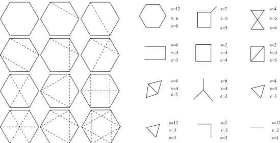
v=3 e=6 v=5 e=5 v=4 e=3 v=3 e=1 v=2 e=6 e=5 v=5 e=4 v=4 e=3 v=4 e=3 e=2 v=6 s=4 v=4 e=5 v=4 e=3 v=3 s=12 s=2 s=2 s=4 s=12 s=2 s=6 s=4 s=12 s=4 s=2
Figure 1: Graphical enumeration/interpretation of the contribution of T rA6
to the partition function. On the left are drawn all possible identifications, schematized by complete dashed graphs. On the right identification has been carried out. The numbers of symmetries, vertices and edges are given for each graph.
where the sum is over unlabelled admissible graphs H, mk(H) is the number
of solid k-cycles and nk(H) the number of solid segments on k + 1 vertices.
See figure 1 for the example of T rA6.
4.3
Exponentiation
Computations on a sheet of paper are more economical using admissible graphs, but systematic machine enumeration is best carried out using nor-malized sequences.
If is not difficult to convince oneself that the notion of connectedness of nor-malized sequences or of admissible graphs is the same, and coincides with the notion of connectedness used to establish eq.(2). We infer that
U (z) = z +Pc Hs(H)1 p e(H)zv(H)Q kt mk(H) k s nk(H) k , where Pc
H is the sum over unlabelled connected admissible graphs or
equiv-alently that U (z) = z + X v,l,{m•,n•} zvpl˜t m• • ˜sn•• m•!n•!M c v,l,{m•,n•},
where ˜tm• • s˜n•• ≡ Q k ¡tk 2k ¢mk¡sk 2 ¢nk and Mc
v,l,(mk,nk) is the number of normal-ized connected sequences.
5
Finite connectivity large N behaviour
Our aim is to use the identities eqs.(1,2) and their consequence eq.(3) to derive mean field type identities valid in the limit N ջ ∞, pN, tk, sk being
N independant, or more generally having finite limits for large N . It is customary to define α≡ limN ջ∞pN .
5.1
Caveat
In this regime, when tk = sk = 0 for all k’s (the Erd¨os-Renyi model), the
event that a graph contains a component with much more edges than ver-tices has a vanishingly small probability, and the connected components look locally like trees. This is called the dilute regime. In particular, the complete graph (a caricature of a non dilute graph) has a negligible weight in the dilute regime.
We are looking for an analogous regime for the perturbed Erd¨os-Renyi model. However, in that case, the complete graph has weight
w = qN (N −1)/2ePktk2k((N −1)k+(−)k(N −1))+
P
ksk2 N (N −1)k.
Compare this to a union of isolated vertices (a caricature of a dilute graph), which has weight w = 1. Consider for instance, the case when there is only one nonvanishing perturbation parameter, say s3. The two weights are
equal if qes3(N −1) = 1. That this crude balance gives the correct qualitative frontier between a dilute regime and a dense regime is confirmed by numerical simulations.
If p≡ α/N and s3 < 0, the complete graph is indeed strongly suppressed
(in fact much more drastically than for the pure Erd¨os-Renyi model). How-ever, if s3 > 0, the weight of the complete graph submerges the weight of
dilute configurations.
To summarize, the following discussion makes sense only if SI does not
become positive and large (≫ N2) for non dilute configurations. An easy
way to ensure that is to take the sign of all perturbations negative. Another possibility would be to take only a finite number of nonzero perturbations, and then impose that the dominant one be negative.
5.2
Main equations
With these observations in mind, we start from ZN = N ! I dy yN +1e U (y) = (1− p)N (N −1)2 N ! I dx xN +1e W (x) and eW (x) = √1 2πβ Z +∞ −∞ e−2˻z2+U (xez− ˻ 2) dz. Recall that p = q/(1 + q) = 1 − e−˻. We fix p = p
N ≡ α/N where α is
a constant, and make changes of variables y ջ y/p, x ջ x/q in the above integrals. In the expansions
U (y/p) =Pc H ¡˺ N ¢E(H)−V (H) eSI(H) yV (H) V (H)! and W (x/q) =Pc H ¡ ˺ N −˺ ¢E(H)−V (H) eSI(H) xV (H) V (H)!
the sum is over connected graphs, and by Euler formula, E − V = L − 1 where L≥ 0 is the number of loops. Hence we may write formaly
U (y/p) = N αu(y) + o(N ) W (x/q) = N αw(x) + o(N ), where u(y) =P T eSI(T ) y V (T ) V (T )! and w(x) = P T eSI(T ) x V (T )
V (T )! are sums over trees
(connected graphs with L = 0). If we use a na¨ıve version of the saddle point approximation and write ZN = eN F +o(N ), we find
F = −1 − logy∗ α + 1 αu(y ∗) (5) F = −α 2 − 1 − log x∗ α + 1 αw(x ∗) (6) w(x) = −zˆ 2 2 + u(xe ˆ z), (7)
where the x∗, y∗ and ˆz are appropriate saddle point values :
α = x∗w′(x∗) = y∗u′(y∗) z = xeˆ zˆu′(xezˆ).
We end this section with the following remarks. The average number of edges is more or less the variable conjugate to p. More precisely, the average number of edges is
q ∂
∂q log¡(1 − p)
−N(N−1)/2Z N¢ .
We infer that in the thermodynamic regime with N ջ ∞ and pN = α/N ,
the average number of neighbors of a given point (i.e. 2/N times the average number of edges) is
c = α + 2α∂F
∂α (8)
For the pure Erd¨os-Renyi model, the weights form a probability distribution, ZN = 1, F = 0, and c = α. In the perturbed models, α is not so easily
measured on the graph, and only the parameter c has direct physical meaning. From the point of view of quantum field theory, it is natural to view α as the bare connectivity and c as the physical connectivity. For each coupling constant tk or sk, it would be desirable to find analogous physical quantities
that first, one can compute directly on a random graph without knowing a priori the sampling measure and that second one can reduce tk or sk to first
order in perturbation theory. This is very ambiguous and we have not found an elegant way to select such physical observables systematically.
5.3
Discussion
We have seen before that a dilute regime for the perturbed Erd¨os-Renyi model with fixed values of the tk’s and sk’s cannot exist if SI becomes large
positive for graphs with many loops. Here we discuss a related limitation even if one considers only loopless graphs.
Instead of considering the complete graph, look at the star shaped tree on n vertices, whose adjacency matrix we denote by S, with a center connected to the n − 1 other vertices. From T rS = 0, kSk = T rS2 = 2(n − 1),
kS2k = n(n − 1) and S3 = (n− 1)S, it is easy to compute recursively that
T rS2k+1 = 0 andkS2k+1k = 2(n−1)k+1 for k ≥ 0, and that T rS2k = 2(n−1)k
and kS2kk = n(n − 1)k for k ≥ 1. As an example, consider again the case
when there is only one nonvanishing perturbation parameter, say s3. The
contribution of star shaped trees to w isP
n (n−1)!1 es3(n−1)
2
xn. As all trees give
a positive contribution to w, no compensation is possible and we conclude that if s3 > 0, the series for w has a vanishing radius of convergence. So it
is meaningless to deform contours, and eq.(6) is meaningless as well. Then so is eq.(5) because analyticity of u(y) at small y implies analyticity of w(x) at small x via eq.(7). On the other hand, if s3 < 0, the star-shaped trees of
large size are very strongly suppressed. Let us note however as shown in the next section that, in the realm of formal power series, eq.(7) describes the correct combinatorial relationship between u and w even if both series have a vanishing radius of convergence.
More generally, if SI(T )/V (T ) is bounded above (an easy way to ensure
be to take only a finite number of nonzero perturbations, and then impose that the dominant one be negative) , w is analytic near the origin. Indeed, if SI(T )/V (T ) ≤ τ for all trees, using the fact that there are nn−2 labelled
trees on n vertices, we see that 0 < wn
n! ≤ nn−2
n! e̍ n, leading to a nonzero radius
of convergence.
For instance, when the sign of every perturbation is negative, the radius of convergence is a nonincreasing function of the tk’s and sk’s : it gets larger
and larger as the tk’s and sk’s get more negative. To see that it remains finite,
consider the linear graph on n vertices, whose adjacency matrix we denote by L. For this graph, for fixed k and large n, T rLk and kLkk grow at most
linearly with n : they count k steps walks, and if the starting point is given, at each step there are at most two choices, so there is the obvious upper bound n2k. There are n!/2 ways to label the linear graph (the symmetry group is
of order 2). So the contribution of the linear trees to w decreases at most geometrically with the size. As all trees give a nonnegative contribution, w has its first singularity on the real positive axis, and at a finite distance.
In the situation when w has a finite radius of convergence, we conclude that there is a forest-like regime for the perturbed Erd¨os-Renyi model that extends the forest-like regime of the pure Erd¨os-Renyi model, and that it is described by the equations eqs.(5,6,7), at least in the small α phase. We shall elaborate on this point in the sequel.
5.4
Combinatorial remarks
As we have seen before, the above formulæ for the free energy rely on crucial assumptions. What we would like to show in this subsection, before embark-ing on a detailed discussion of analytic features of these equations, is that the combinatorics embodied in eq.(7) is correct. Suppose that we forget about the random graph model for a moment, and consider instead a random forest model, w being the generating function for random weighted trees.
Expand the function u(xez) in powers of z : u(xez) = P
lz l l! ¡x d dx ¢l u(x). It is well-known from quantum field theory that the formal expansion of
Z dze1~ “ −z2 2 +u(xez) ”
is a weighted sum of all connected Feynmann graphs. The weight of a Feyn-mann graph is computed as follows : each edge gives a factor ~ (propagator), each vertex of degree l gives a factor ~−1¡x d
dx
¢l
u(x) and finally one divides by the order of the symmetry group of the graph. The logarithm is given by the same sum, but restricted to connected graphs. For connected graphs,
the power of ~ is the number of loops minus 1, so the dominant contribution in the small ~ limit restricts the sum to connected loopless graphs, i.e. trees. On the other hand, the small ~ limit is given by the saddle point approxima-tion, i.e. eq.(7). So w is a sum over all trees, each vertex of degree l giving a factor ¡x d
dx
¢l u(x).
But u(x) itself is a tree generating function, so ¡xd dx
¢l
u(x) is the gener-ating function for trees with l marked vertices (a vertex can be marked more than once). So eq.(7) means that to construct w, one takes arbitrary trees, (call them naked trees) and then blows up every vertex of degree l into a new tree with l marked vertices from which naked edges emerge. Note that a naked vertex can be blown up in a trivial tree, corresponding to the term x in u(x) = x +⋅ ⋅ ⋅.
As we have emphasized before, if T is a tree, each term t in the expansion of eSI(T )in terms of matrix elements of the adjacency matrix A of T defines a subgraph of T i.e. a forest with the same vertex set as T , edge {i, j} ∈ E(T ) being present in the forest if and only if the term t contains the factor Aij or
Aji. But the connected components of the forest being given, one reconstructs
w by connecting the different components with appropriate edges. This is exactly the procedure described by eq.(7) if w is the generating function for eSI(T ) and u the one for eSI(T ).
5.5
Effective model
If we have the original model in mind, each uk is itself a highly nontrivial
kind of partition function. However, if we take each uk as an independent
parameter, we can make a rather general analysis. In fact, there is a simple model for which the uk’s are the fundamental microscopic parameters in the
sense that they appear directly in the definition of the weights. We call this model an effective model for the following reasons.
In quantum field theory, the term “effective” often means that one re-nounces to deal with all observables of a system and only concentrates on certain degrees of freedom, so that the other ones can be averaged. For in-stance, to compute the long distance behaviour, one first averages over the short distance fluctuations. We are going to do something analogous here : we renounce to observe the local structure of connected components and are only interested in the distribution of their size. So instead of keeping track of the weight of each detailed connected component, we can as well give all components of a given size the same weight, namely the average weight given by the original model for components of that size.
an effective weight u(ef f )(H) = pE(H)c
k for any connected graph H of size
k, and assume multiplicativity, so that for an arbitrary graph u(ef f )(H) =
pE(H)Q
kc nk(H)
k where nk(H) is the number of components of size k of H.
If we trade ck for λkck, we multiply the weight u(ef f )(H) by a trivial factor
λV (H) so we shall assume that the c
k’s are normalized by c1 = 1 (the special
case c1 = 0 would need a separate treatment). Define the corresponding
effective weight w(ef f )(G) = qE(G)P
H,E(H)⊂E(G)u(ef f )(H)p−E(H), where the
sum is over all graphs on the same vertex set as G whose edge set is a subset of that of G. Note that contrary to the weight u(ef f ), the weight
w(ef f )(G) does in general depend on the detailed structure of the graph,
and not only on the sizes of connected components. Our interest however is in the distribution of sizes of connected component of graphs of large size N ջ ∞ sampled using the weight w(ef f ). Following the same steps
as for the original model, we find that this distribution can be obtained in the thermodynamic limit from tree generating functions u(ef f ) and w(ef f )
satisfying the very same coupled equations eqs.(5,6,7) as the original u and w. The coefficients of u(ef f ) are very simple in terms of c1, c2,⋅ ⋅ ⋅ because all components of the same size have the same weight, and by Caley’s theorem there are kk−2 trees on k vertices. Hence u(ef f ) = P
k≥1 k
k−2
k! cky
k. Hence if
one sets ck = k2−kPT ∈TkeSI(T ) where the sum is over trees of size k, the
effective model has the same component size distribution as the original one. For all these reasons, we shall remove in the sequel the superscript (ef f )
from u(ef f )and w(ef f ), even if we sometimes keep the distinction between the
weights u and w and the effective weights u(ef f )and w(ef f ). Accordingly, we
shall analyse eqs.(5,6,7), which involve only the component size distribution, without making explicitly the distinction between the original model and the effective model.
5.6
Connected components and percolation
We return to the finite N arbitrary p case to start the argument. As Wk is,
modulo an overall multiplicative factor, the total weight of connected graphs of size k, we infer from eq.(1) that the mean number of connected components on k vertices is Nk = Wk ZN ∂ZN ∂Wk = N ! k!(N − k)!Wk ZN −k ZN (1− p)N (N −1)−(N−k)(N−k−1)2 .
Taking into account that when pN = α, p(N − k) = α(1 − k/N), we find that in the dilute regime, for fixed k and N ջ ∞, ZN −k
ZN ∼ e
−k(F +˺∂F
(1− p)N (N −1)−(N−k)(N−k−1)2 ∼ e−k˺ so that
Nk/N ∼
wk k!α
k−1e−k(˺+F +˺∂F∂˺).
As expected, in this regime only trees contribute thermodynamically to the finite components.
From these equations for the abundance of connected component of each size, we can easily derive a percolation criterion. Indeed, by construction, P
kkNk/N = 1, but what about the approximate sum
X k kwk k!α k−1e−k(˺+F +˺∂F ∂˺) ?
For each fixed k and N ջ ∞, the kth term is a good approximation to
kNk/N , but there is problem of inversion of limits. Physically, the
approxi-mate sum counts the fraction of points in components of finite size, so it is ≤ 1.
If we assume that u is analytic at small y, then F is analytic and small at small α and w is analytic and small at small x. Moreover, x∗ is an increasing
function of α at small α. From eq.(6), we infer that F + α∂F
∂˺ = −α −
log x˺∗ or equivalently, αe−˺−F −˺∂F∂˺ = x∗. Then P
kk wk k!αk−1e −k(˺+F +˺∂F ∂˺) = x∗
˺w′(x∗) = 1 for small enough α. However, it may happen that as a function
of α, x∗ = αe−˺−F −˺∂F∂˺ is non monotonic. There may be a value αc such that x∗ increases in the interval [0, α
c] but then starts to decrease, so that
x∗(α) ≤ x∗(α
c) in some interval strictly containing [0, αc]. One could build
models where x∗(α) has several oscillations, but in the sequel, we concentrate
on the first. For a given α, denote by ¯α ≤ αc the small solution to the
equation x∗(α) = x∗(¯α). Then we obtain the more general result that finite
components occupy a fraction x˺∗w′(x∗) = ˺¯
˺ ≤ 1 of the sites in the system.
If α > αc, something else than finite components, in fact on general grounds
one single giant component, occupies a fraction 1 − ˺¯
˺ vertices. Thus, the
percolation criterion is that αe−˺−F −˺∂F∂˺ is maximum at α = αc. So the transition point is when
α + 2α∂F ∂α + α
2∂2F
∂α2 = 1 (9)
The first two terms yield simply the true average connectivity c = α+2α∂F ∂˺, it
would be nice to have a direct physical interpretation of the third term α2 ∂2F
∂˺2. This percolation criterion is expressed solely in terms of the free energy as a function of α. But it can also be related to analytic properties of w. Indeed,
the relevant saddle point equation is α = x∗w′(x∗). As α approaches αc, x∗ reaches a maximum, so that the x∗ derivative of x∗w′(x∗) has to get large, diverging at α = αc. If αc is finite, this means that w and w′ are finite at
α = αc, but w′′ is infinite. If the coefficients of w are non negative2, this
means that x∗(α
c) is the radius of convergence of w. From x∗(αc), we recover
αc itself by the general saddle point equation α = x∗w′(x∗).
Suppose now (we shall soon argue that this is true in many cases including interesting ones) that even if x∗(α
c) is the radius of convergence of w, the
function u is not singular at y∗(α
c). Hence u allows to compute the free
energy F and show that it is analytic in some interval strictly containing αc.
From that point of view, we observe that the saddle point equations imply that x∗ = y∗e−˺ = y∗e−y∗u′(y∗)
from which the percolation criterion, i.e. the determination of the maximum of x∗ becomes
y∗ ∂α ∂y∗ = y
∗u′(y∗) + y∗2u′′(y∗) = 1. (10)
In the same spirit, the true average connectivity can be expressed as c = y∗u′(y∗) + 2− 2 u(y
∗)
y∗u′(y∗).
In general, if u has nonegative coefficients and eq.(10) has a solution strictly within the disc of convergence, one can go through the above argu-ment in the reverse order to prove the existence of a percolation transition with the announced characteristics. This is the case for instance if u is an en-tire function with nonnegative coefficients, or more generally if u is function with nonnegative coefficients such that u′′ is unbounded when the argument
approaches the radius of convergence. It is worth to observe that if the y expansion of u has nonnegative coefficients, then the same is true of the x expansion of w. Indeed, from eq.(7) and the corresponding saddle point equation we infer that xw′(x) = ˆz. Hence as functions of x, w and ˆz have
the same singular points, and
w′(x) = exw′(x)u′(xexw′(x)).
Expand both sides of this identity to see that w1 = 1 and that wk+1− uk+1
is a polynomial in u1 = 1, u2,⋅ ⋅ ⋅ , uk, w1 = 1, w2,⋅ ⋅ ⋅ , wk with nonnegative
coefficients.
In the case of our original model, the situation is more tricky. We know by construction that the x expansion of w has nonnegative coefficients, but to ensure the existence of a dilute regime, the same cannot be true in general of u. In the sequel, we shall see that in perturbation theory at any finite order,
2
This should be the case in statistical mechanics, and it is true by construction for our initial model as long as the parameters are real.
we are in the following situation : the coefficients of u may be negative, but nevertheless u′(y) is analytic (in fact a polynomial) and positive in a interval
strictly containing 0 and a solution of eq.(10). Then our previous arguments can be made rigorous and there is a (perturbative) percolation transition with the announced characteristics. We do not know if this argument can be extended outside the realm of perturbation theory. The numerical sim-ulations are encouraging, but the behaviour of some perturbative series is puzzling. Before discussing that, let us consider three simple but significant examples.
6
Three easy examples
6.1
The case of the Erd¨
os-Renyi model
Let us recover the Erd¨os-Renyi model in this framework. In that case, by construction, U (y) = u(y) = y and y∗ = α. Eq.(5) leads to F = 0 for all
val-ues of α (no surprise, for the Erd¨os-Renyi model the weights are normalized as a probability distribution). Then eq.(7) leads to ˆz = xezˆ, and from the
Lagrange inversion formula,
ˆ z =X k kk−1 k! x k w=X k kk−2 k! x k
which are the classical (rooted and non rooted) tree generating functions (in fact, this gives a proof of Caley’s formula for the number of trees). Note that if we use naively eq.(6), we can deduce that F = 0 only for α≤ 1.
The number of connected components of size k is Nn ∼ Nk
k−2
k! αk−1e−k˺,
which is well-known to be true for fixed k and large N , for any value of α. Notice again that the use of u plays a crucial role in our approach. Using only w, we would get the component distribution only for α≤ 1. In fact, for the corresponding random forest model (which is thermodynamically equivalent to the random graph model for α ≤ 1) limN ջ∞Nn/N is k
k−2
k! αk−1e−k˺ for
α ≤ 1 but is nonanalytic at α = 1, which is the percolation transition. The total number of points belonging to components of size k is ∼ Nkk−1 k! αk−1e−k˺. For α≤ 1,P kk k−1 k! α ke−k˺ = α, but for α > 1,P kk k−1 k! α ke−k˺ = ¯α, where ¯
α is the smallest solution to αe−˺ = ¯αe−¯˺. The giant component occupies
6.2
The nested Erd¨
os-Renyi model
As another example, suppose that u(ef f )(H) = pE(H) for all graphs, i.e that
ck = 1, k ≥ 1. Then w(ef f )(G) = qE(G)PH,E(H)⊂E(G)1 = (2q)E(H). Both
weights describe the Erd¨os-Renyi model, but with different values for the probability of an edge. Going to the large N finite connectivity limit, we find u =P
k≥1 k
k−2
k! yk, and from our previous analysis of the Erd¨os-Renyi model,
we find that yu′(y) =P
k≥1 kk−1
k! y
k is the Lambert function L(y), the solution
of L(y)e−L(y) = y analytic close to 0 and vanishing at 0. Hence ˆz = L(xezˆ),
so that ˆze−ˆz = xezˆ. Hence 2ˆz = L(2x). Moreover, from u(y) = L(y)− L(y)2
2
we find 2w(ef f )(x) = L(2x)− L(2x)2
2 . So we recover the doubling of the edge
probability when passing from the u(ef f ) weight to the w(ef f ). The u(ef f )
percolation transition is at α = 1 but the w(ef f )percolation transition occurs
at α = 1/2. Note that the equation y∗u′(y∗) = L(y) = α cannot be solved for α ≥ 1, but that the free energy F = α/2 and the true connectivity c = 2α have an analytic continuation for larger α’s. That this analytic continuation is the true value of F cannot in principle be decided from our arguments (we would have to do one more step of the same construction to view the u(ef f ) weight itself as a composite weight). But this does not prevent us
from finding and analysing correctly the w(ef f ) transition, because it occurs
strictly before the u(ef f ) transition.
6.3
The matching model
When uk = 0 for k ≥ 2 we recover the Erd¨os-Renyi model, so let us try the
next degree of difficulty, when uk = 0 for k ≥ 3 but u2 is a free parameter.
Thus w(ef f )(G) is the generating function for a gas of disjoint egdes on G,
that is, the generating function for (all, non necessarily maximal) matchings on G. This is a rather natural weight from the point of view of combinatorics. It is plain that the detailed structure of G is relevant, and not simply the size of its connected components. On the other hand, the u(ef f ) weight is
nonzero only for a finite number of connected graphs, so that the function U(ef f ) is simply U(ef f ) = z + qu
2z 2 2 and ZN = N ! H dz zN +1ez+qu2 z2 2 . In such a simple case, the saddle point approximation applies without subtleties, and we retrieve, in the large N finite connectivity limit, the expected equations. The function w(x) does not seem to be an elementary function. The small x and the perturbative small u2 expansions are straightforward but become
quickly ugly. However from u = y + u2y
2
2 , we can easily find the percolation
criterion. Parametrizing u2 = 1−y2y2c
eq.(10), one finds that at the percolation threshold : y∗ = yc αc = 1 + yc 2 cperc= 1 + yc 2 + 1− yc 1 + yc .
So αc decreases from 1 to 1/2 when u2 grows, but the physical average
con-nectivity cperc increases from 1 to 3/2. The special case u2 = 1 is of special
combinatorial significance, because the weight w(ef f )(G) counts the number
of configurations of non adjacent edges on G. Then yc = 1/2, αc = 3/4 and
cperc = 13/12. Consequently, xc = 12e−3/4, from which we can derive a result
of direct combinatorial significance : 1 N ! X T ∈TN # matchings of T ∼ Cst¡2e 3/4¢N N5/2 , to be compared with N !1 P T ∈TN1 = NN −2 N ! ∼ 1 √ 2̉ eN
N5/2. Hence, if we put the uniform probability law on labelled trees of size N , the average number of matchings on a random tree of size N behaves like Cst¡16
e
¢N/4 .
7
Back to the original model
7.1
Finite orders in perturbation theory
Remember that we established in section 4.3 that U (z) = z +Pc Hs(H)1 pe(H)zv(H) Q kt mk(H) k s nk(H) k , wherePc
H is the sum over unlabelled connected admissible graphs (we could
equivalently reason in terms of normalized connected sequences). Consider the coefficient of Q
kt mk
k s nk
k : it is the sum over admissible graphs with mk
solid k-cycles and nk solid segments on k + 1 vertices. There is only a finite
number of ways to join these fixed solid components with any number of complete dashed graphs. So the coefficient of Q
kt mk
k s nk
k is a polynomial in p
and z. A fortiori, if we restrict to admissible graphs H such that v = l + 1, which are the ones contributing to u, the sum is finite, and the coefficent of Q
kt mk
k s nk
k in the perturbative expansion of u(y) is a polynomial in y.
Note that u(y) = y + O(y2), so yu′(y) = y + O(y2) and yu′(y) + y2u′′(y) =
y + O(y2), where the O(y2) vanish to zeroth order in perturbation theory.
Hence to any finite order in perturbation theory, yu′(y) is analytic and
in-creasing up in a large value of y, but yu′(y) + y2u′′(y) = 1, the signal of the
to any finite order in perturbation theory our initial model exhibits a perco-lation transition described by our previous results. In the following we shall make explicit perturbative computations of the free energy, the percolation threshold, etc, for the special case tk = 0, sk = 2µδk,3. To compare with
the prediction of the Molloy-Reed criterion, we need first to show how to compute it in perturbation theory for our model.
7.2
Moments of the degree distribution, Molloy-Reed’s
criterion
By degree distribution of a given labelled graph G on N vertices is meant the sequence (n0(G), n1(G),⋅ ⋅ ⋅ , nN −1(G)) where ni(G) is the number of vertices
in G with exactly i neighbours. For fixed N , the Molloy-Reed model concen-trates on the set of all those labelled graphs with a fixed degree distribution (n0, n1,⋅ ⋅ ⋅) and gives them uniform probability, see [6]. This represents a
mi-crocanonical point of view in the sense that the degree distribution is fixed and can not fluctuate. For a grand canonical presentation of the same idea, see [2]. If, for large N , (n0/N, n1/N,⋅ ⋅ ⋅) converges (in a sense made precise
by Molloy and Reed) to a probability distribution (f0, f1,⋅ ⋅ ⋅), a limiting
ran-dom graph model is obtained, which depends only on (f0, f1,⋅ ⋅ ⋅) and not on
the details of the approximating sequence (n0/N, n1/N,⋅ ⋅ ⋅). We now recall
the percolation criterion for the Molloy-Reed model with arbitrary degree distribution.
For a given graph G, define k(q)(G) as the following average over vertices of
G : k(q)(G)≡ 1 N N X i=1 li(G)q.
For instance, when q = 1, N k(G) = 2E(G). The statistical average hkqi ≡ 1
P
Gw(G)
P
Gw(G)k(q)(G) is called the q-th
moment of the degree distribution. Note that in the Molloy-Reed model, all graphs have the same degree distribution, so that hkqi = k(q)(G) for all G in
the relevant statistical ensemble.
The Molloy-Reed percolation criterion states that the Molloy-Reed random graph has a giant component if and only if the two first moments of the degree distribution verify hk2− 2ki > 0. For the Erd¨os-Renyi model, hki =
α,hk2i = α(α + 1), leading to the percolation threshold α = 1.
Our present purpose is to compute in perturbation theory the first moments of the degree distribution for our model. In principle, it is possible to compute
hkqi for any q ≥ 1. In the definition hkqi = N Z1 N X G∈GN eSI(G)w 0(G) X i,j1,⋅⋅⋅,jq aij1⋅ ⋅ ⋅ aijq of the q-th moment, eSI(G)P
i,j1,⋅⋅⋅,jqaij1⋅ ⋅ ⋅ aijq may be viewed as the x deriva-tive taken at x = 0 of exp³SI(q)(G, x)´≡ exp³SI(G) + xPi,j1,⋅⋅⋅,jqaij1⋅ ⋅ ⋅ aijq
´ . Seen as a new term of interaction, this exponential is still multiplicative and permutation invariant. We thus follow the steps which led us to eq.(2) (see sec. 3.2) to prove thathkqi is the derivative taken at x = 0 of(N −1)!
ZN H dz zN +1eU (q)(z) = 1 N ZN(q) ZN , where Z (q)
N is the partition function of the model obtained from the
original model by replacing SI by SI(q). In the large N limit, we proceed just
as in sec. 5.2 to show that ZN(q) = eN Fq+o(N ), F
q being the new free energy :
Fq = −1 − log y⋆ q ˺ + 1 ˺u (q)(y⋆
q). In this expression, u(q) is the tree generating
function for the new model and y⋆
q is the corresponding saddle point.
We now take the derivative and put x = 0 to yield hkqi = 1 α X T X i,j1,⋅⋅⋅,jq eSI(T )a ij1⋅ ⋅ ⋅ aijq yV (T ) V (T )!
Just as we did in the original model, we can use normalized sequences (or admissible graphs) to give a combinatorial interpretation of the over-lined term. A sequence i1j1⋅ ⋅ ⋅ injn is said to be normalized with respect to
{mk, nk}, q if
• n = q +P
kk (mk+ nk),
• 1 comes before 2, which comes before 3,... which comes before the number v of distinct elements among the sequence,
• i1 6= j1,⋅ ⋅ ⋅ , in6= jn,
• it has a correct structure. That is, the sequence of the 2(n − q) first terms has a correct structure as regards T r and k k and, moreover, in = in−1 =⋅ ⋅ ⋅ = in−q+1.
We putMv,l,(mk,nk),q for the number of such sequences. Finally, the q-th moment of the degree distribution is
hkqi = y ⋆ α + 1 α X v,{m•,n•} ˜ tm• • ˜sn•• m•!n•!M t v,(mk,nk),qy ⋆v (11)
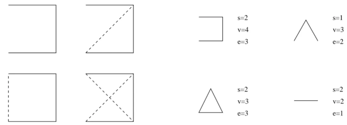
s=1 s=2 s=2 s=2 v=3 e=1 e=2 e=3 v=4 e=3 v=3 v=2
Figure 2: Graphical representation for the coefficients of s3.
In particular, the Molloy-Reed’s criterion can, in principle, be computed by means of this formula : it involves normalized sequences (of type (mk, nk))
to which are concatenated subsequences of 2 elements for hki or 3 elements for hk2i.
We now study a simple example in which all quantities mentioned above can be explicitly (although perturbatively) computed.
7.3
Perturbation theory :
the example
tk
= 0, sk
=
2µδk,3
This is the simplest non-trivial case for which sk 6= 0. The weight of a graph
G is
w(G) = pE(G)(1− p)−E(G)e̅Pijklaijajkakl.
According to our previous discussion, we assume that µ < 0. To get the percolation criterion, we use the general theory exposed in the preceding section. We set Mt
n,m ≡ Mcn,n−1,m. The definition of y∗ is y∗u′(y∗) = α, i.e.
y∗+X n,m ny∗nµ m m!M t n,m = α.
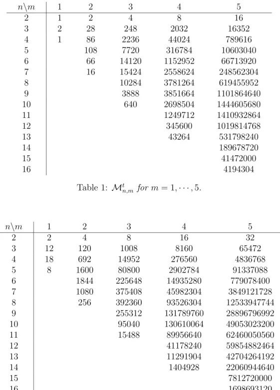
In fact, we were not able to find an expression of Mt
n,m valid for all
n, m, and we rely on a direct enumeration, up to order 6, of the normalized sequences, see table [1] for the first five orders. At this moment, a fully automated enumeration algorithm starting from scratch and working in a reasonnable time would need too much memory. To have some control over possible errors coming from human input, we have checked our results with two independent algorithms. On a 2.5 Ghz processor, the computation of the
fifth order takes about 5 minutes, but the sixth order takes about 8 hours : the growth in complexity is extremely rapid, at least factorial.
Up to third order in µ, y⋆ takes the following form:
y⋆ = α− 2α2(α + 1)(2α + 1)µ + 2α2(−1 − 17α − 56α2− 57α3− 15α4
+4α5)µ2− 4 3α
2(1 + 81α + 788α2 + 2485α3+ 3303α4+ 1808α5
+159α6− 126α7+ 8α8)µ3+⋅ ⋅ ⋅
The percolation criterion states that there exists a giant connected com-ponent if y∗u′(y∗) + y∗2u′′(y∗) > 1 and that, on the contrary, all connected components are of finite size if y∗u′(y∗) + y∗2u′′(y∗) < 1. With u(y) = y +P
n,mMtn,m ̅m
m!y
n, the boundary between the percolating region and the
non percolating region is a curve in the (α, µ) plane, of equation :
α− 1 +X n,m n(n− 1)y∗nµ m m!M t n,m = 0 (12)
We can solve this equation for α as a perturbative series in µ. Up to order 5, this yields αperc = 1− 26µ + 336µ2− 9500 3 µ 3+49718 3 µ 4 −9913285 µ5−41436164 15 µ 6+ ⋅ ⋅ ⋅ (13) Putting α = αpercin formula (8) we find that, at the percolation threshold,
the mean number of neighbours of a given vertex is
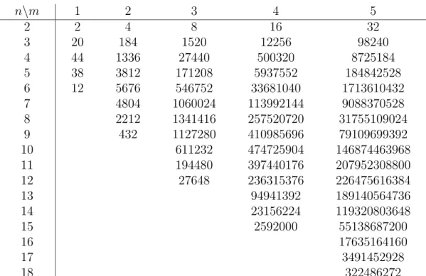
cperc= 1− 10µ − 50µ2− 652 3 µ 3 −19786 3 µ 4 −3498268 15 µ 5 −67025012 9 µ 6+ ⋅ ⋅ ⋅ (14) In the preceding section, we saw how to infer the moments of the degree distribution from enumeration of the appropriate normalized sequences. Ta-bles [2] and [3] show the result of these enumerations for hki and hk2i.
We compute hki (either by means of formula (8) or using the enumeration [2] together with eq.(11)) andhk2i as perturbative series in µ, and then solve
the equation hk2− 2ki = 0 in α to find
αM R = 1− 24µ + 274µ2− 7324 3 µ 3+28708 3 µ 4 −577988 3 µ 5 + ⋅ ⋅ ⋅ , which does not coincide with αperc.
n\m 1 2 3 4 5 2 1 2 4 8 16 3 2 28 248 2032 16352 4 1 86 2236 44024 789616 5 108 7720 316784 10603040 6 66 14120 1152952 66713920 7 16 15424 2558624 248562304 8 10284 3781264 619455952 9 3888 3851664 1101864640 10 640 2698504 1444605680 11 1249712 1410932864 12 345600 1019814768 13 43264 531798240 14 189678720 15 41472000 16 4194304 Table 1: Mt n,m for m = 1,⋅ ⋅ ⋅ , 5. n\m 1 2 3 4 5 2 2 4 8 16 32 3 12 120 1008 8160 65472 4 18 692 14952 276560 4836768 5 8 1600 80800 2902784 91337088 6 1844 225648 14935280 779078400 7 1080 375408 45982304 3849121728 8 256 392360 93526304 12533947744 9 255312 131789760 28896796992 10 95040 130610064 49053023200 11 15488 89956640 62460050560 12 41178240 59854882464 13 11291904 42704264192 14 1404928 22060944640 15 7812720000 16 1698693120 17 171051008
n\m 1 2 3 4 5 2 2 4 8 16 32 3 20 184 1520 12256 98240 4 44 1336 27440 500320 8725184 5 38 3812 171208 5937552 184842528 6 12 5676 546752 33681040 1713610432 7 4804 1060024 113992144 9088370528 8 2212 1341416 257520720 31755109024 9 432 1127280 410985696 79109699392 10 611232 474725904 146874463968 11 194480 397440176 207952308800 12 27648 236315376 226475616384 13 94941392 189140564736 14 23156224 119320803648 15 2592000 55138687200 16 17635164160 17 3491452928 18 322486272
Table 3: Enumeration of the sequences appearing in hk2i.
8
Discussion and perspectives
In this paper, we have studied a class of perturbations of the Erd¨os-Renyi model which introduce correlations between the edges : the weight of a graph depends on the abundance of certain geometric features.
To solve this model, we have introduced an auxiliary model whose tree generating function u was expected to present better convergence properties than the original one w. The free energy F in the large N limit has been determined and a percolation transition has been established by means of an effective model : the percolation criterion is given by an equation, either on F or on u. We also have formulæ for the degree distributions.
On the basis of these general results we give explicit formulæ for the above quantities in the particular case where all parameters but one vanish. These perturbative results raise some crucial questions. Indeed, we hope that the thermodynamical model makes sense for µ < 0 but that µ > 0 has to be discarded because it gives too much weight to strongly connected configura-tions and cannot be treated like a diluted, tree-like, regime. In fact, up to sixth order, it is not so clear that the series for αperc is actually convergent
for negative µ, because its general term increases very fast. However, as sug-gested by the fifth and sixth terms, we hope that the following terms may
all be negative, the series hence being possibly summable when µ < 0. This interpretation is supported by the form of the perturbative expansion (14) of the physical connectivity parameter cperc, which seems much better behaved,
with negative coefficients for orders ¿0.
We also have computed the Molloy-Reed criterion, which does not give an appropriate description of the percolation transition in this model. The µ expansion of αM R seems to present the same pathology as αperc. A possibility
is that this series is indeed divergent for negative µ : the equation hk2− 2ki
may not admit any solution in α as soon as µ < 0. Another possibility is that, just as for αperc the series may stop to alternate at higher orders. Anyway, it
would be desirable to determine a class of models for which the Molloy-Reed criterion is valid, and we believe that a minimal requirement may be a kind of locality. Indeed, the Molloy-Reed criterion concentrates on the first two moments of the degree distribution, which are local quantities in the sense that k(q)(G) can be computed as soon as the immediate environment of each
vertex is known, independently of how the vertices are connected to each other. Even in the simple model that we used to illustrate perturbation the-ory, this information is not sufficient to compute the weight of a graph : one must also know the immediate environment of the first neighbours of each vertex.
Finally, we also believe that a more thorough understanding of degree corre-lations induced by attacks deserves a systematic treatment.
References
[1] R. Albert and A.-L. Barab´asi, Statistical mechanics of complex networks, Reviews of Modern Physics 74, 47 (2002).
[2] M. Bauer and D. Bernard, Maximal entropy random networks with given degree distribution, ArXiv:cond-mat/0206150
[3] M. Bauer and 0. Golinelli, Random incidence matrices : moments of the spectral density, ArXiv:cond-mat/0007127
[4] S. N. Dorogovtsev and J.F.F. Mendes, Evolution of Networks, Adv. Phys. 51, 1079, (2002).
[5] P. Erd¨os and A. R´enyi, On the evolution of random graphs, Publ. Math. Inst. Hungar. Acad. Sci. 5 (1960), 17–61.
[6] M. Molloy and B. Reed, Statistical mechanics of complex networks, Ran-dom Struct. Algorithms 6, 161, (1995); and Comb. Proba. Comput. 7, 295, (1998).
[7] D. S. Callaway, M. E. J. Newman, S. H. Strogatz and D. J. Watts, Net-work robustness and fragility : Percolation on random graphs, Phys. Rev. Lett. 85, 5468-5471 (2000).
[8] R. Cohen, K. Erez, D. ben-Avraham and S. Havlin, Breakdown of the Internet under intentional attack, Phys. Rev. Lett 86, 3682 (2001)