HAL Id: hal-02950523
https://hal.archives-ouvertes.fr/hal-02950523
Submitted on 8 Oct 2020
HAL is a multi-disciplinary open access
archive for the deposit and dissemination of
sci-entific research documents, whether they are
pub-lished or not. The documents may come from
teaching and research institutions in France or
abroad, or from public or private research centers.
L’archive ouverte pluridisciplinaire HAL, est
destinée au dépôt et à la diffusion de documents
scientifiques de niveau recherche, publiés ou non,
émanant des établissements d’enseignement et de
recherche français ou étrangers, des laboratoires
publics ou privés.
atmospheric inversion
R. Thompson, F. Chevallier, A. Crotwell, G. Dutton, R. Langenfelds, R.
Prinn, R. Weiss, Y. Tohjima, T. Nakazawa, P. Krummel, et al.
To cite this version:
R. Thompson, F. Chevallier, A. Crotwell, G. Dutton, R. Langenfelds, et al.. Nitrous oxide emissions
1999 to 2009 from a global atmospheric inversion. Atmospheric Chemistry and Physics, European
Geosciences Union, 2014, 14 (4), pp.1801-1817. �10.5194/ACP-14-1801-2014�. �hal-02950523�
www.atmos-chem-phys.net/14/1801/2014/ doi:10.5194/acp-14-1801-2014
© Author(s) 2014. CC Attribution 3.0 License.
Atmospheric
Chemistry
and Physics
Nitrous oxide emissions 1999 to 2009 from a global atmospheric
inversion
R. L. Thompson1, F. Chevallier2, A. M. Crotwell3,11, G. Dutton3, R. L. Langenfelds4, R. G. Prinn5, R. F. Weiss6, Y. Tohjima7, T. Nakazawa8, P. B. Krummel4, L. P. Steele4, P. Fraser4, S. O’Doherty9, K. Ishijima10, and S. Aoki9
1Norwegian Institute for Air Research, Kjeller, Norway
2Laboratoire des Sciences du Climat et de l’Environnement, Gif sur Yvette, France 3NOAA ESRL, Global Monitoring Division, Boulder, CO, USA
4Commonwealth Scientific and Industrial Research Organisation, Aspendale, Australia 5Center for Global Change Science, MIT, Cambridge, MA, USA
6Scripps Institution of Oceanography, La Jolla, CA, USA 7National Institute for Environmental Studies, Tsukuba, Japan
8Center for Atmospheric and Oceanic Studies, Graduate School of Science, Tohoku University, Sendai 980-8578, Japan 9Atmospheric Chemistry Research Group, School of Chemistry, University of Bristol, Bristol, UK
10Japan Agency for Marine-Earth Science and Technology, Yokohama, Japan
11Cooperative Institute for Research in Environmental Sciences, University of Colorado, Boulder, CO, USA
Correspondence to: R. L. Thompson ([email protected])
Received: 22 March 2013 – Published in Atmos. Chem. Phys. Discuss.: 13 June 2013 Revised: 8 January 2014 – Accepted: 9 January 2014 – Published: 17 February 2014
Abstract. N2O surface fluxes were estimated for 1999 to
2009 using a time-dependent Bayesian inversion technique. Observations were drawn from 5 different networks, incor-porating 59 surface sites and a number of ship-based mea-surement series. To avoid biases in the inverted fluxes, the data were adjusted to a common scale and scale offsets were included in the optimization problem. The fluxes were calcu-lated at the same resolution as the transport model (3.75◦ lon-gitude × 2.5◦latitude) and at monthly time resolution. Over the 11-year period, the global total N2O source varied from
17.5 to 20.1 Tg a−1N. Tropical and subtropical land regions were found to consistently have the highest N2O emissions,
in particular in South Asia (20 ± 3 % of global total), South America (13 ± 4 %) and Africa (19 ± 3 %), while emissions from temperate regions were smaller: Europe (6 ± 1 %) and North America (7 ± 2 %). A significant multi-annual trend in N2O emissions (0.045 Tg a−2N) from South Asia was
found and confirms inventory estimates of this trend. Consid-erable interannual variability in the global N2O source was
observed (0.8 Tg a−1N, 1 standard deviation, SD) and was largely driven by variability in tropical and subtropical soil fluxes, in particular in South America (0.3 Tg a−1N, 1 SD)
and Africa (0.3 Tg a−1N, 1 SD). Notable variability was also found for N2O fluxes in the tropical and southern oceans
(0.15 and 0.2 Tg a−1N, 1 SD, respectively). Interannual
vari-ability in the N2O source shows some correlation with the
El Niño–Southern Oscillation (ENSO), where El Niño con-ditions are associated with lower N2O fluxes from soils and
from the ocean and vice versa for La Niña conditions.
1 Introduction
Nitrous oxide (N2O) is now the third largest contributor to
anthropogenic radiative forcing among the long-lived green-house gases (GHGs) and has a global warming potential of approximately 300 times that of CO2(Forster et al., 2007).
N2O also plays an important role in stratospheric ozone
de-pletion through the formation of NO and, with the decrease in chlorofluorocarbon (CFC) emissions, is the dominant ozone-depleting substance currently emitted (Ravishankara et al., 2009). Emissions of N2O have been increasing since the
pre-industrial era due to human activities, leading to sub-stantial increases in the atmospheric mole fraction, from
270 nmol mol−1(abbreviated as ppb; 1 nmol = 10−9mol) to
around 323 ppb today (WMO, 2011). N2O emissions occur
naturally as a byproduct of the processes of denitrification (microbial reduction of nitrate and nitrite) and nitrification (microbial oxidation of ammonia), which occur in soils and in the ocean. Several human activities enhance nitrification and denitrification rates and, consequently, emissions of N2O
to the atmosphere. The most significant of these activities is food production through the use of nitrogen fertilizers, ma-nure, and land cultivation (Syakila and Kroeze, 2011), with smaller contributions from bio-fuel production (Crutzen et al., 2008). There are also direct N2O emissions from
indus-try, combustion and municipal waste (Denman et al., 2007). Atmospheric monitoring of N2O started in the late 1970s
and has been instrumental in determining long-term emis-sion trends (Syakila and Kroeze, 2011), and more recently with improved data precision, in determining the spatial dis-tribution of emissions (Hirsch et al., 2006; Huang et al., 2008). Superimposed on the long-term trend in atmospheric N2O, is considerable interannual variability in the growth
rate. To date, there have been only a few studies that have tried to understand the mechanisms driving this variability (Nevison et al., 2007, 2011; Thompson et al., 2013). On the one hand, the growth rate is influenced by changes in non-emission related variables, such as atmospheric transport, especially stratosphere-to-troposphere transport, which car-ries N2O-depleted air from the stratosphere into the
tropo-sphere and has a significant influence on the observed N2O
seasonal cycle and also contributes to interannual variability (Nevison et al., 2011). On the other hand, it is known from in situ flux measurements that terrestrial biosphere fluxes of N2O are strongly determined by climatological factors such
as soil temperature, moisture and precipitation (Bouwman et al., 2002; Skiba and Smith, 2000; Smith et al., 1998). A num-ber of land ecosystem models now include the nitrogen cycle and simulate N2O fluxes (Potter et al., 1996; Zaehle et al.,
2010), but owing to the non-linear response of N2O
produc-tion to soil and climate parameters, as well as to nitrogen substrate availability, the modelled fluxes are associated with large uncertainties (Werner et al., 2007). Some ecosystem models predict a significant N2O soil-flux–climate link. In
a study by Xu et al. (2012) the sensitivity of N2O emissions
to soil temperature was found to be 1 Tg of N equivalents of N2O (abbreviated Tg N) per kelvin per year. A study by
Za-ehle et al. (2011) also found a strong link between N2O soil
emissions and climate. It has not been possible, however, to verify modelled interannual variability in the N2O flux, since
sufficient long-term in situ flux measurements are not avail-able. Therefore, to learn more about interannual variability in N2O fluxes, and especially the integrated response at
re-gional or continental scales of N2O flux to climate forcing, it
is useful to turn to atmospheric observations.
Numerous multi-annual flux studies have been carried out for the other important GHGs, CO2 (Bousquet et al.,
2000; Rayner et al., 1999; Rödenbeck et al., 2003) and CH4
(Bousquet et al., 2006; Chen and Prinn, 2006), using atmo-spheric observations and the inversion of atmoatmo-spheric trans-port. These flux studies found the land–atmosphere fluxes of both these species to be significantly sensitive to climate variability and in particular to the El Niño–Southern Oscil-lation (ENSO) climate variation and to the climate impacts of the Pinatubo eruption (Bousquet et al., 2006; Chen and Prinn, 2006; Peylin et al., 2005; Rödenbeck et al., 2003). To the best of our knowledge, no previous multi-annual inver-sion study of this type has been conducted for N2O. In this
study, we focus on N2O fluxes from 1999 to 2009, since
the data precision improved greatly during the 1990s and since a number of new sites became operational in the late 1990s and early 2000s. The inversions were run from 1996 to 2009, but we only examine the data from 1999 since the first 3 years of simulation were needed for spin-up. (The long spin-up time was required to achieve realistic tropospheric and stratospheric mole fractions, which depend on the sur-face source, the stratospheric sink and the rate of air mass exchange across the tropopause.)
In this paper, we first describe the inversion method and atmospheric transport model used, as well as provide details on the atmospheric observations that were included (Sect. 2). Second, we describe a number of tests that were performed for the sensitivity of the observation network to changes in N2O emissions and for the sensitivity of the inversions to
their prior emission estimates (Sects. 2.6 and 2.7, respec-tively). In Sects. 3 and 4, we discuss the results of the in-versions and the variability and trends in the retrieved N2O
emissions.
2 Inversion method
2.1 Bayesian inversion
In this study, we used a Bayesian inversion method to find the optimal surface fluxes at monthly temporal resolution and at the same spatial resolution as the atmospheric transport model (i.e. 3.75◦×2.5◦longitude by latitude). The inversion is performed in two time intervals: from 1996 to 2003 and 2002 to 2009. The first 3 years of the first period and the first 2 years of the second period were used for spin-up. (A 2-year spin-up time was considered sufficient for the second pe-riod, since the initial conditions for 2002 from the first period were reused in the second period). According to the Bayesian method, the optimal solution (in this study, the surface fluxes and the initial mole fractions), x, is that which provides the best fit to the atmospheric observations, y, while remaining within the bounds of the prior estimates, xb, and their
un-certainties (for details about the Bayesian method refer to Tarantola, 2002). The extra constraint of the prior prevents the problem from being ill-conditioned in the mathematical sense. Based on Bayesian theory, as well as Gaussian-error
hypotheses, one can derive the following cost function:
J (x) = (x − xb)TB−1(x − xb) + (H (x) − y)TR−1(H (x) − y)
, (1)
where the flux uncertainties are described by the error covari-ance matrix, B; the observation uncertainties are described by the error covariance matrix, R; and H is a non-linear operator for atmospheric transport and chemistry (in Eq. 1, the matrix transpose is indicated byT). To solve this equation, we used the variational framework of Chevallier et al. (2005). In this approach, the minimum of J (x) is found iteratively using a descent algorithm based on the Lanczos version of the conju-gate gradient algorithm (Lanczos, 1950). This algorithm re-quires several computations of the gradient of J with respect to x (where H is the linearized form of the transport operator,
H):
∇J (x) = B−1(x − xb) +HTR−1(H (x) − y). (2)
For problems with a very large number of variables, it is not possible to directly define H or HTowing to numerical lim-itations. Therefore, the elements of HT are found implicitly via the adjoint model of the atmospheric transport and chem-istry (Chevallier et al., 2005; Errico, 1997).
2.2 Transport model
The inversion framework relies on the offline version of the Laboratoire de Météorologie Dynamique version 4 (LMDz) general circulation model (Hourdin and Armengaud, 1999; Hourdin et al., 2006). This version computes the evolution of atmospheric compounds using archived fields of winds, convection mass fluxes and planetary boundary layer (PBL) exchange coefficients that have been built from prior inte-grations of the complete general circulation model, which was nudged to ECMWF ERA-Interim winds (Uppala et al., 2005). The LMDz model is on a 3-D Eulerian grid consist-ing of 96 zonal columns, 73 meridional rows and 19 hybrid pressure levels. The daytime PBL is resolved by 4–5 levels, the first of which corresponds to 70 m altitude and the other levels spaced between 300 and 500 m apart from there on upwards. Above the PBL the mean resolution is 2 km up to a height of 20 km, above which there are four levels with the uppermost level at 3 hPa. Tracer transport is calculated in LMDz using the second-order finite-volume method of Van Leer (1977) and is described for LMDz by Hourdin and Ar-mengaud (1999). Turbulent mixing in the PBL is parame-terized using the scheme of Mellor and Yamada (1982) and thermal convection is parameterized according to the scheme of Tiedtke et al. (1989). The offline LMDz was run with a physical time step of 30 min. For the calculation of J and its gradient ∇J (Eqs. 1 and 2), the tangent linear H and ad-joint HToperators were coded from the offline LMDz ver-sion (Chevallier et al., 2005).
In the case of N2O, the sink in the stratosphere needs to be
accounted for. Losses of N2O occur via photolysis and
reac-tion with O(1D) accounting for 90 % and 10 % of the sink, re-spectively (Minschwaner et al., 1993). These reactions were included in the forward and adjoint models of the atmo-spheric transport as described in Thompson et al. (2011). The number density of O(1D) and the photolysis rate were de-fined for each grid cell and time step and were taken from prior simulations of the coupled global circulation and at-mospheric chemistry model LMDz-INCA (Hauglustaine et al., 2004) with the same transport fields as used in the inver-sion. The fields of photolysis rate from LMDz-INCA were scaled by a factor of 0.66 to give a mean total annual loss of N2O of 12.2 Tg a−1N, consistent with estimates of N2O
life-time between 124 and 130 years (Prather et al., 2012; Volk et al., 1997). This was necessary as the fields from LMDz-INCA had not been previously optimized for use in N2O
in-versions, and without this scaling the lifetime would have been circa 84 years.
2.3 Prior flux estimates
Our a priori N2O flux estimate (xbin Eqs. 1 and 2) was
com-piled from different models/inventories for
– terrestrial biosphere fluxes, including natural and cul-tivated ecosystems;
– anthropogenic emissions, from fossil and bio-fuel combustion, industry, and municipal waste;
– biomass burning emissions;
– coastal and open ocean fluxes.
The terrestrial biosphere fluxes were provided from the ni-trogen version of the ORCHIDEE land surface model (O-CN, version 0.74, Zaehle and Friend, 2010). O-CN accounts for nitrogen input from atmospheric deposition, biological nitrogen fixation and fertilizer usage and simulates nitrogen losses via leaching, nitrification and denitrification pathways, and emissions of trace gases to the atmosphere. The model is driven by climate data (CRU-NCEP) and interannually vary-ing N inputs. Data were originally provided at 3.75◦×2.5◦ (longitude by latitude) and monthly resolution. For the an-thropogenic emissions (excluding direct agricultural emis-sions, which are accounted for in O-CN), we used EDGAR-4.1 (Emission Database for Global Atmospheric Research) inventory data. These data were provided at 1.0◦×1.0◦and annual resolution. Since N2O emissions from these sources
are small relative to the terrestrial biosphere and ocean sources, and because they have relatively little seasonal-ity, annual resolution is considered sufficient. The biomass burning emissions were provided by the Global Fire Emis-sions Database (GFED-2.1) at 1.0◦×1.0◦and monthly res-olution (van der Werf et al., 2010). For the ocean fluxes, we used estimates provided by the ocean biogeochemistry model PISCES, which was embedded in a climate model but was not constrained by meteorological data; thus interannual
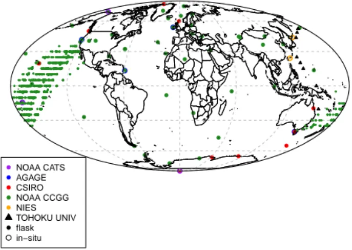
NOAA CATS AGAGE CSIRO NOAA CCGG NIES TOHOKU UNIV flask in−situ
Fig. 1. Map of observation sites and ship tracks by network.
ALT CCGG ALT CSIRO ASC CCGG ASK CCGG AZR CCGG BAL CCGG BKT CCGG BME CCGG BMW CCGG BRW CCGG BRW CATS BSC CCGG CBA CCGG CFA CSIRO CGO AGAGE CGO CCGG CGO CSIRO CHR CCGG COI NIES CRZ CCGG CYA CSIRO EIC CCGG ESP CSIRO GMI CCGG HAT NIES HBA CCGG HUN CCGG ICE CCGG IZO CCGG KEY CCGG KUM CCGG KZD CCGG KZM CCGG LEF CCGG MAA CSIRO MHD AGAGE MHD CCGG MID CCGG MLO CCGG MLO CSIRO MQA CSIRO NMB CCGG NWP TOHOKU NWR CCGG PAL CCGG PSA CCGG PTA CCGG RPB AGAGE RPB CCGG SEY CCGG SHM CCGG SIS CSIRO SMO AGAGE SMO CCGG SMO CATS SPO CCGG SPO CSIRO SPO CATS STM CCGG SUM CCGG SYO CCGG TAP CCGG TDF CCGG THD AGAGE THD CCGG UTA CCGG UUM CCGG WIS CCGG WLG CCGG ZEP CCGG 1999 2000 2001 2002 2003 2004 2005 2006 2007 2008 2009 2010 Year <2 2 − 4 5 − 8 9 − 30 >30
Fig. 2. N2O observation availability at individual sites for the in-version period 1999 to 2009. The legend indicates the number of observations per month.
variations may not be in phase with observations (Dutreuil et al., 2009). Data were provided at 1.0◦×1.0◦and monthly resolution. (See Table 3 for the global N2O emission from
each source.)
2.4 Observations
Atmospheric observations were pooled from a number of global networks, independent sites and ship-based measure-ments (see Figs. 1 and 2 and Table 1). Long-term records of N2O mole fraction are available from the Advanced Global
Atmospheric Gases Experiment (AGAGE, http://cdiac.ornl. gov/ftp/ale_gage_Agage/AGAGE/) and the NOAA Halocar-bons and other Atmospheric Trace Species (HATS, http: //www.esrl.noaa.gov/gmd/hats/), including both the OTTO and the Chromatograph for Atmospheric Trace Species (CATS, http://www.esrl.noaa.gov/gmd/hats/insitu/cats/) pro-grammes, which were established in the 1990s. The early data, however, cannot be used to constrain regional fluxes of N2O owing to the less precise instrumentation available
at that time. During the 1990s significant improvements to the measurement technique were made and, thus, sufficiently precise data from these networks are available from the mid-to late 1990s. Both the AGAGE and CATS networks consist of stations equipped with in situ gas chromatographs with electron capture detectors (GC-ECD) to measure the dry air mole fraction of N2O (ppb) and provide measurements at
approximately 40 min intervals. The AGAGE data are re-ported on the SIO1998 scale and have an uncertainty on in-dividual measurements of about 0.1 ppb (Prinn et al., 2000), while the NOAA CATS data are reported on the NOAA2006 scale and have an uncertainty of about 0.3 ppb (Hall et al., 2007). In the late 1990s and early 2000s, NOAA also estab-lished a flask network under the Carbon Cycle and Green-house Gases (CCGG, http://www.esrl.noaa.gov/gmd/ccgg/) programme. Flask samples from this network are also anal-ysed by GC-ECD in a central laboratory and are reported on the NOAA2006A scale. These data have an uncertainty of 0.4 ppb based on the mean value of differences from paired flasks. There is some concern that there could be a calibra-tion shift between NOAA CCGG data collected before and after 2001, owing to a poor calibration routine used prior to 2001. To test for the influence of this shift on the re-trieved fluxes, we include an inversion test in which mini-mal NOAA CCGG data are included (test IAVR; see sec-tion 2.7 for details). The Commonwealth Scientific and In-dustrial Research Organisation (CSIRO) in Australia have also operated a flask network since the early 1990s (data available from the World Data Centre for Greenhouse Gases, http://ds.data.jma.go.jp/gmd/wdcgg/). These measurements are reported on the NOAA2006 scale with an uncertainty of approximately 0.3 ppb for each flask measurement (Francey et al., 2003). In addition, we included data from two sta-tions operated by the National Institute for Environmental Science (NIES) in Japan, which operate in situ GC-ECDs (Tohjima et al., 2000) (data available from the World Data Centre for Greenhouse Gases, http://ds.data.jma.go.jp/gmd/ wdcgg/). These data are reported on NIES’s own scale, which is approximately 0.6 ppb lower than NOAA2006A for ambi-ent concambi-entrations as determined from an intercomparison of
NOAA standards (see http://www.esrl.noaa.gov/gmd/ccgg/ wmorr/results.php?rr=rr5¶m=n2o). Lastly, we include data from ship-based flask measurements in a programme op-erated by Tohoku University, Japan (data available from the World Data Centre for Greenhouse Gases, http://ds.data.jma. go.jp/gmd/wdcgg/) (Ishijima et al., 2009). Comparisons with NOAA standards indicate that the Tohoku measurements are approximately 0.2 ppb higher than the NOAA2006A scale. (For a list of all stations and their locations, see Table 1.)
Gradients of N2O mole fraction in the atmosphere, which
provide information about the distribution of N2O fluxes, can
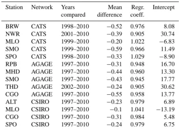
be small and of the same order of magnitude as the calibra-tion offsets between different scales and networks. For this reason, it is of critical importance to correct for these offsets prior to and/or in the inversion. Corazza et al. (2011) incorpo-rated the optimization of calibration offsets into their inver-sion problem, thereby reducing the bias that these have on the retrieved fluxes. We adopt the same approach as Corazza et al. (2011), but, in addition, we corrected the observations based on our prior estimated calibration offsets before run-ning the inversion. Using both approaches means that the in-version will only “fine-tune” the offsets, thereby limiting the degrees of freedom that can be used for this adjustment. Prior calibration offsets were estimated relative to NOAA CCGG (NOAA2006A scale) based on the comparison of observa-tions from two or more networks at the same location, e.g. in American Samoa, where NOAA CATS, NOAA CCGG and AGAGE all have measurements. Overlaps between NOAA CCGG and AGAGE also exist at MHD, CGO, RPB and THD, as well as between NOAA CCGG and CSIRO at ALT, MLO, CGO and SPO, where the data were corrected to the NOAA2006A scale using the linear trend and offset calcu-lated at each site (see Table 2). At sites where there was no overlap, the mean of the corrections applied to other sites within the same network was used. For NIES, which has no overlap with other networks, a temporally fixed offset was used and was based on shared cylinder intercomparisons with NOAA CCGG (Y. Tohjima, personal communication, 2012). The comparisons of AGAGE and NOAA CCGG data show a significant trend in the offset (0.02–0.04 ppb a−1), which is consistent at all compared sites and points to a possible cal-ibration drift in the scales relative to each other. However, without further detailed investigation it is not possible to tell how much each scale may have drifted and in which direc-tion, but this drift could be significant when considering N2O
emission trends.
All data were filtered for suspicious values using flags set by the data providers. Additionally, the data were filtered for outliers, which were defined as points outside 2 standard de-viations (SD) of the running mean calculated over a window of 45 days for flask data and 3 days for in situ data. The win-dow lengths were optimized on a trial basis to ensure that only suspicious values were removed.
Observations from sites with in situ GC-ECDs were se-lected for the afternoon (12:00 to 17:00) if they were
low-altitude sites (< 1000 m a.s.l.) and for the night (00:00 to 06:00) if they were mountain sites (> 1000 m a.s.l.). These data selection criteria were chosen to minimize the impact of boundary layer vertical transport errors in the model. In general, data were assimilated at hourly resolution. For flask data, no selection was applied and data were assimilated when available. For the ship-based data (from Tohoku Uni-versity), one observation was assimilated per grid cell and time step, and where more than one observation was avail-able, the values were averaged. This was done to avoid as-similating highly correlated observations (observation error correlations are not taken into account; see Sect. 2.5.2). 2.5 Specification of uncertainties
2.5.1 Prior flux error covariance matrix
A key aspect of the Bayesian inversion is the description of prior flux uncertainty. This uncertainty is described by the error covariance matrix, B (in Eqs. 1 and 2), in which the diagonal elements are the error variances in each grid cell and time step and the off-diagonal elements are the covari-ances. Unfortunately, there are insufficient observations of N2O flux to be able to accurately determine the error
vari-ances and covarivari-ances. Therefore, a simple approach for this was used; that is, we calculated the variance of each land grid cell as the maximum flux for the year found in the eight surrounding grid cells plus the cell of interest. Choosing the maximum value from nine grid cells allows the inversion to change the small-scale spatial pattern of the fluxes. For ocean grid cells, the errors were adjusted to 100 % of the flux in the given grid cell; this is different to the land ap-proach to avoid overestimating the errors in ocean grid cells along coastlines. The errors calculated for land in the South-ern Hemisphere were scaled by 0.66 owing to the weaker observational constraint in this hemisphere and to allow for greater reliance on the prior estimates. Both land and ocean errors were set to a maximum of 0.44 g m−2a−1N and min-imum of 0.03 g m−2a−1N. In areas covered by sea ice, the error was reduced by a factor of 100. The covariance was cal-culated as an exponential decay with distance and time using correlation scale lengths of 500 km over land and 1000 km over ocean and 12 weeks, respectively. The correlation scale length of the errors in land fluxes depends strongly on the source; here we chose 500 km as an educated guess to repre-sent the correlation of the errors in the spatially diffuse soil emission, which is the dominant source and is modulated by land use, soil type, moisture and temperature, as well as by the amount of nitrogen input. The choice of 12 weeks for the temporal correlation length was to represent the correlation of fluxes within a season on a sub-continental scale, while at the same time, flux time steps 12 months apart only have a correlation of 0.02, so the posterior fluxes will not be strongly dependent on the prior interannual variability. The whole er-ror covariance matrix was then scaled so that its sum was
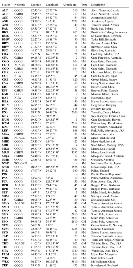
Table 1. Observation sites used in the inversions. Sites in bold type were included in the reference data set. (FM stands for flask measurement,
CM for continuous measurement, and SM for ship-based flask measurement.)
Station Network Latitude Longitude Altitude (m) Type Description
ALT CCGG 82.45◦N 62.52◦W 210 FM Alert, Nunavut, Canada
ALT CSIRO 82.45◦N 62.52◦W 210 FM Alert, Nunavut, Canada
ASC CCGG 7.92◦S 14.42◦W 54 FM Ascension Island, UK
ASK CCGG 23.18◦N 5.42◦E 2728 FM Assekrem, Algeria
AZR CCGG 38.77◦N 27.38◦W 40 FM Terceira Island, Azores
BAL CCGG 55.35◦N 17.22◦E 7 FM Baltic Sea, Poland
BKT CCGG 0.2◦S 100.32◦E 865 FM Bukit Koto Tabang, Indonesia
BME CCGG 32.37◦N 64.65◦W 30 FM St. Davis Head, Bermuda
BMW CCGG 32.27◦N 64.88◦W 30 FM Tudor Hill, Bermuda
BRW CCGG 71.32◦N 156.6◦W 11 FM Barrow, Alaska, USA
BRW CATS 71.32◦N 156.6◦W 11 CM Barrow, Alaska, USA
BSC CCGG 44.17◦N 28.68◦E 3 FM Black Sea, Romania
CBA CCGG 55.2◦N 162.72◦W 21 FM Cold Bay, Alaska, USA
CFA CSIRO 19.28◦S 147.05◦E 2 FM Cape Ferguson, Australia CGO CCGG 40.68◦S 144.68◦E 164 FM Cape Grim, Tasmania
CGO AGAGE 40.68◦S 144.68◦E 164 CM Cape Grim, Tasmania
CGO CSIRO 40.68◦S 144.68◦E 164 FM Cape Grim, Tasmania CHR CCGG 1.7◦N 157.17◦W 3 FM Christmas Island, Kiribati
COI NIES 43.15◦N 145.5◦E 45 CM Cape Ochi-ishi, Japan
CRZ CCGG 46.45◦S 51.85◦E 120 FM Crozet Island, France CYA CSIRO 66.28◦S 110.53◦E 60 FM Casey Station, Australia
EIC CCGG 27.15◦S 109.45◦W 50 FM Easter Island, Chile
ESP CSIRO 49.38◦N 126.55◦W 39 FM Estevan Point, Canada
GMI CCGG 13.43◦N 144.78◦E 2 FM Mariana Island, Guam
HAT NIES 24.05◦N 123.8◦E 10 CM Hateruma, Japan
HBA CCGG 75.58◦S 26.5◦W 30 FM Halley Station, Antarctica HUN CCGG 46.95◦N 16.65◦E 344 FM Hegyhatsal, Hungary
ICE CCGG 63.25◦N 20.29◦W 118 FM Heimay, Iceland
IZO CCGG 28.3◦N 16.48◦W 2360 FM Tenerife, Canary Islands
KEY CCGG 25.67◦N 80.2◦W 3 FM Key Biscayne, Florida, USA
KUM CCGG 19.52◦N 154.82◦W 3 FM Cape Kumukahi, Hawaii
KZM CCGG 43.25◦N 77.88◦E 2519 FM Plateau Assy, Kazakhstan KZD CCGG 44.06◦N 76.82◦E 601 FM Sary Taukum, Kazakhstan
LEF CCGG 45.93◦N 90.27◦W 868 FM Park Falls, Wisconsin, USA
MAA CSIRO 67.62◦S 62.87◦E 32 FM Mawson, Australia
MHD AGAGE 53.33◦N 9.9◦W 25 CM Mace Head, Ireland
MHD CCGG 53.33◦N 9.9◦W 25 FM Mace Head, Ireland
MID CCGG 28.22◦N 177.37◦W 4 FM Sand Island, Midway, USA MLO CCGG 19.53◦N 155.58◦W 3397 FM Mauna Loa, Hawaii
MLO CSIRO 19.53◦N 155.58◦W 3397 FM Mauna Loa, Hawaii MQA CSIRO 54.48◦S 158.97◦E 12 FM Macquarie Island, Australia
NMB CCGG 23.58◦S 15.03◦E 456 FM Gobabeb, Namibia
NWP TOHOKU – – – SM Northwest Pacific, Japan
NWR CCGG 40.05◦N 105.58◦W 3526 FM Niwot Ridge, CO, USA
PAL CCGG 67.97◦N 24.12◦E 560 FM Pallas, Finland
POC CCGG – – – SM Pacific Ocean Shipboard
PSA CCGG 64.92◦S 64◦W 10 FM Palmer Station, Antarctica
PTA CCGG 38.95◦N 123.73◦W 55 FM Point Arena, CA, USA
RPB AGAGE 13.17◦N 59.43◦W 45 CM Ragged Point, Barbados RPB CCGG 13.17◦N 59.43◦W 45 FM Ragged Point, Barbados
SEY CCGG 4.67◦S 55.17◦E 3 FM Mahe Island, Seychelles
SHM CCGG 52.72◦N 174.1◦E 40 FM Shemya Island, Alaska SIS CSIRO 60.08◦N 1.25◦W 30 FM Shetland Island, UK
SMO AGAGE 14.25◦S 170.57◦W 42 CM Tutuila, American Samoa
SMO CCGG 14.25◦S 170.57◦W 42 FM Tutuila, American Samoa SMO CATS 14.25◦S 170.57◦W 42 CM Tutuila, American Samoa
SPO CCGG 89.98◦S 24.8◦W 2810 FM South Pole, Antarctica
SPO CSIRO 89.98◦S 24.8◦W 2810 FM South Pole, Antarctica SPO CATS 89.98◦S 24.8◦W 2810 CM South Pole, Antarctica
STM CCGG 66.0◦N 2.0◦E 7 FM Ocean Station M, Norway
SUM CCGG 72.58◦N 38.48◦W 3238 FM Summit, Greenland SYO CCGG 69.0◦S 39.58◦E 11 FM Syowa Station, Antarctica
TAP CCGG 36.73◦N 126.13◦E 20 FM Tae-ahn Peninsula, Korea TDF CCGG 54.87◦S 68.48◦W 20 FM Tierra del Fuego, Argentina THD AGAGE 41.05◦N 124.15◦W 107 CM Trinidad Head, CA, USA
THD CCGG 41.05◦N 124.15◦W 107 FM Trinidad Head, CA, USA UTA CCGG 39.9◦N 113.72◦W 1320 FM Wendover, Utah, USA UUM CCGG 44.45◦N 111.1◦E 914 FM Ulaan Uul, Mongolia
WIS CCGG 31.13◦N 34.88◦E 400 FM Sede Boker, Israel WLG CCGG 36.27◦N 100.92◦E 3810 FM Mt Waliguan, China
Table 2. Comparison of different networks with NOAA CCGG at
sites with parallel measurements. The mean difference is calculated
as NOAA CCGG minus other (units of nmol mol−1). The
sion coefficient (slope) and intercept are given for a linear regres-sion of the other network vs. NOAA CCGG.
Station Network Years Mean Regr. Intercept
compared difference coeff.
BRW CATS 1998–2010 −0.52 0.976 8.08 NWR CATS 2001–2010 −0.39 0.905 30.74 MLO CATS 1999–2010 −0.20 1.022 −6.83 SMO CATS 1999–2010 −0.59 0.966 11.49 SPO CATS 1998–2010 −0.33 1.029 −8.90 RPB AGAGE 1997–2010 −0.31 0.948 16.70 MHD AGAGE 1997–2010 −0.44 0.960 13.30 SMO AGAGE 1997–2010 −0.43 0.945 17.77 THD AGAGE 2002–2010 −0.24 0.905 30.62 CGO AGAGE 1997–2010 −0.55 0.958 13.77 ALT CSIRO 1997–2010 −0.23 0.979 6.89 MLO CSIRO 1997–2010 −0.1 1.041 −13.19 CGO CSIRO 1997–2010 −0.31 0.984 5.48 SPO CSIRO 1997–2010 −0.24 0.979 6.75
consistent with an assumed global total prior uncertainty of 2 Tg a−1N.
2.5.2 Observation error covariance matrix
Another key component of the Bayesian inversion is the ob-servation uncertainty, which is described by the error covari-ance matrix, R. A thorough description of the observation error variances is needed to avoid giving too strong weight-ing to very uncertain observations, which becomes particu-larly important if these observations are far from the expected value. The observation error variance takes into account the measurement and transport model errors. Measurement er-rors consist of random and systematic components. Random errors are assessed in determining the measurement repro-ducibility, while systematic errors, such as errors in the cali-bration, instrumentation, air sampling, etc., are more difficult to determine. For the measurement error, we have used the estimates given by the data providers, which includes ran-dom and, as far as is known, systematic errors and is ap-proximately 0.3 ppb (circa 0.1 %). For the transport model errors, we have estimated two contributions: (1) transport er-rors (following Rödenbeck et al., 2003) and (2) erer-rors from a lack of subgrid-scale variability (following Bergamaschi et al., 2010), both of which were calculated using forward model simulations run with the same prior fluxes and mete-orology as the inversions. The first error uses the 3-D mole fraction gradient around the grid cell where the site is located as a proxy for the transport error, and thus strong vertical and/or horizontal gradients lead to large error estimates. The second error uses the change in mole fraction in the grid cell integrated over the e-folding time for flushing the grid cell with the modelled wind speed. This is used as a proxy for the influence of not accounting for the homogeneous distribution
of fluxes within the grid cell and their location relative to the observation site (for details, see Bergamaschi et al. 2010). For observations from southern mid- to high-latitude sites, we have included an additional transport error to account for the fact that LMDz cannot accurately reproduce the sea-sonal cycle at these latitudes owing largely to errors in South-ern Hemisphere stratosphere-to-troposphere transport. This is seen in a phase shift of the simulated vs. observed sea-sonal cycles of N2O and CFC-12. Both these species have a
stratospheric sink and tropospheric mixing ratios influenced by seasonal stratosphere-to-troposphere transport. This error was estimated to be approximately 1.0 ppb. We did not ac-count for correlations between errors, i.e. R is a diagonal matrix.
2.6 Forward model sensitivity tests
One major motivation of this study is to determine whether or not N2O emissions vary interannually on a regional scale,
driven, for example, by ENSO climate variability. There-fore, it is important to first ascertain whether such a flux signal can be detected by the current observational network. Since ENSO largely affects the tropics, in particular tropical and temperate South America, we focus on a hypothetical flux signal from this region. We performed forward model simulations to test the influence of low/high fluxes during 1 year in tropical and subtropical South America (1 Tg a−1N less/more evenly distributed over land than in the prior) on atmospheric N2O mole fractions in an El Niño year (1998)
and a La Niña year (1999), respectively. (The results of these tests are presented in Sect. 3.1.)
2.7 Inversion sensitivity tests
We ran five different inversion scenarios to test the robustness of the results to the observations used and to the inversion setup (see Table 4). Observation data contain gaps; in other words the data coverage is not consistent throughout the in-version period (see Fig. 2). Furthermore, some observation sites only became operational a few years after the start year of the inversion. The inconsistent data coverage over time re-sults in varying degrees of constraint on the fluxes in space and time; therefore in periods with good data coverage, a stronger constraint on the fluxes is possible, whereas when there is poorer data coverage, the fluxes are closer to the prior. Hence, to examine interannual variations in the fluxes, it is necessary to distinguish between variations owing to in-consistent data coverage and those resulting from the atmo-spheric signal. Thus ran a set of inversions with as consistent as possible data coverage (the reference data set) and a set of inversions using all available observation sites. For the refer-ence data set inversions, 15 sites were included, these having data throughout the inversion period and no gaps of longer than 6 months, while for the other inversions, 59 sites were included and no gap criterion was applied (see Table 1 for
Table 3. N2O sources used in the a priori fluxes (totals shown for 2005).
Source type Data set Resolution Total (Tg a−1N)
terrestrial biosphere ORCHIDEE O-CN monthly 10.83
– agriculture (direct + indirect) 3.88
– natural soils 6.95
ocean PISCES monthly 4.28
waste water EDGAR-4.1 annual 0.21
solid waste EDGAR-4.1 annual 0.004
solvents EDGAR-4.1 annual 0.05
fuel production EDGAR-4.1 annual 0.003
ground transport EDGAR-4.1 annual 0.18
industry combustion EDGAR-4.1 annual 0.41
residential & other combustion EDGAR-4.1 annual 0.18
shipping EDGAR-4.1 annual 0.002
other sources EDGAR-4.1 annual 0.0005
biomass burning GFED-2.1 monthly 0.71
Total monthly 16.84
Table 4. Overview of inversion sensitivity tests.
Test Prior No. surface No. Measurement
name fluxes sites observations error
CLMR climatology 15 144 849 0.3 ppb
IAVR interannual 15 144 849 0.3 ppb
IAVAa interannual 59 180 057 0.3 ppb
IAVE interannual 59 180 057 0.5 ppb
IAVSb interannual 59 180 057 0.3 ppb
aIAVA is the control run.bIAVS is the same as the control run except that in this test the sink
was also optimized.
the list of sites). The reference data set inversions also serve as a test for the influence of a potential NOAA CCGG scale shift (see Sect. 2.4) as only one NOAA CCGG site was in-cluded in this data set. The reference data set inversions con-sisted of one run using the interannually varying prior fluxes (IAVR) and one run with climatological prior fluxes (CLMR) to test the influence of the assumed flux interannual variabil-ity. For the CLMR run, 1 year of fluxes (2002) was repeated for every year. The other sets of inversions (using all data) were created with interannually varying fluxes and consisted of one run to test the sensitivity of the results to the obser-vation error (IAVE), one test where the stratospheric sink was also included in the optimization (IAVS) according to the method described in Thompson et al. (2011), and a con-trol run (IAVA) (see Table 4 for an overview of the sensitivity tests). (The results of these tests are presented in Sects. 3.2 and 3.3.)
2.8 Calculation of posterior flux errors
From the Lanczos algorithm used to find the gradient of J (x), we also obtain an estimate of the leading eigenvectors of the Hessian matrix J00(x). The number of eigenvectors obtained
equals the number of iterations performed. This fact is par-ticularly useful since the inverse of J00(x) gives the posterior
flux error covariance matrix, A. However, since the eigen-values of J00(x) are the reciprocals of the eigenvalues of A, many iterations are needed to obtain sufficient eigenvalues and eigenvectors to approximate A (Chevallier et al., 2005). Therefore, we use the Monte Carlo approach instead to es-timate the posterior flux errors as described by Chevallier et al. (2007). In this approach, an ensemble of inversions is run with random perturbations in the prior fluxes and observa-tions, consistent with B and R, respectively. The statistics of the ensemble of posterior fluxes are equivalent to the poste-rior uncertainty. For the uncertainty calculation we used an ensemble of 20 inversions of one year (2003) for the ref-erence and full observation data sets. The prior and poste-rior uncertainties given in Table 5 are all calculated from the Monte Carlo ensemble.
3 Results
3.1 Robustness and uncertainty analysis
The current observational network has few sites in tropi-cal regions and, notably, no sites in tropitropi-cal and subtropi-cal South America. However, some constraint on fluxes in this region is obtained from sites in the South Atlantic and equatorial Pacific. From the forward sensitivity tests, sig-nificant differences in atmospheric mole fractions at tropi-cal and subtropitropi-cal sites were found after 2–3 months and globally after circa 6 months following the perturbation. Fig-ure 3 shows the difference in mole fraction (test scenario minus control run) at Samoa and Ascension Island for an El Niño year (low fluxes) and a La Niña year (high fluxes). The current measurement precision on a single flask sample
Table 5. Prior and posterior error (Tg a−1N) and error reduction (ER) calculated from Monte Carlo ensembles for the reference data set (Ref) and all data (All).
Region Error Prior Error Ref ER Ref % Error All ER All %
Global 2.17 0.62 71 0.52 76
North America 0.65 0.50 23 0.45 31
Tropical & South America 1.01 0.89 12 0.84 17
Europe 0.57 0.35 39 0.27 52 North Asia 0.30 0.30 0 0.27 10 South Asia 0.95 0.62 35 0.56 42 Africa 0.96 0.58 40 0.55 43 Australasia 0.26 0.25 3 0.25 4 Ocean 20–90◦N 0.30 0.28 6 0.26 12 Ocean 20◦S–20◦N 0.61 0.51 17 0.48 21 Ocean 90–20◦S 0.53 0.47 11 0.47 12
is approximately 0.3 ppb, so the signal after approximately 6 months (circa 0.2 ppb) will be detectable from the mean of 4 or more flask samples. If the change in flux persists for approximately 1 year, the atmospheric signal in the tropics reaches circa 0.3 ppb compared to 0.15 ppb in the extratrop-ics, for example at Mace Head (53◦N). Given that the
mag-nitude of this signal is similar at all tropical and subtropical sites, the observational network would be sensitive to a re-gional change in fluxes of this magnitude in the tropics.
Figure 4 shows the annual mean error reduction per grid cell calculated as 1 minus the ratio of the posterior to prior flux error, where the posterior error is found from the Monte Carlo ensemble of inversions, for the reference and full ob-servation data sets. As expected, the distribution of error re-duction is strongly dependent on the observational network, with most of the reductions in the temperate northern lati-tudes. Despite the low error reduction at the grid-cell level in the tropics and Southern Hemisphere, modest error reduc-tions are achieved by integrating the fluxes over regions. Ta-ble 5 shows the prior and posterior errors, and error reduction globally and for eight land and three ocean regions. Using all observations, strong error reductions were found for Eu-rope (52 %), North America (31 %), South Asia (42 %) and Africa (43 %), while only moderate error reductions were found for South America (17 %), North Asia (10 %) and Aus-tralasia (4 %). The error reductions using only the reference sites were somewhat smaller, notably so for Europe, North America and South Asia, where new observation sites were established during the inversion period.
3.2 Mean spatial distribution
The mean spatial distribution (1999–2009) of the posterior fluxes did not differ significantly between sensitivity tests, nor did the general distribution of the fluxes change re-markably throughout the 11-year period. For this reason, only the mean flux from the control inversion, IAVA, is shown (Fig. 5). Tropical and subtropical regions exhibited
the highest N2O fluxes, in particular tropical and
subtrop-ical South America (13 ± 4 % of global total), South and East Asia (20 ± 3 %), and tropical and subtropical Africa (19 ± 3 %) (Table 6). High fluxes were also found for Europe (6 ± 1 %), mostly in central Europe, and temperate North America (7 ± 2 %), predominantly in the eastern states. This distribution is not unexpected, and a similar pattern is also seen in the prior fluxes. All inversions, however, increased the flux relative to the prior in South and East Asia, and to a lesser extent in tropical Africa, North America, tropical South America and southern Europe (Fig. 6). In contrast, the inversions slightly reduced the mean flux in southern Africa, southern South America, and in the Great Lakes region of North America.
Emissions from India and eastern China were found to be considerably more important than predicted in the prior. This may be due to an underestimate of mineral nitrogen fer-tilizer application rates. These rates having been increasing rapidly in recent years; however, in the prior model the fer-tilizer rates from 2006 to 2009 were based on 2005 statistics, and thus agricultural emissions in latter years may be under-estimated in the prior. Another contributing factor may be an underestimate of reactive nitrogen deposition rates; for in-stance, deposition rates of NOy(an important denitrification
substrate) are known to be systematically underestimated in India (Dentener et al., 2006). In general, both India and China have very high rates of NO3(HNO3and nitrate aerosol) and
NH+4 and NH3 deposition, which has likely also increased
in recent years owing to increased nitrogen fertilizer usage and industrial activities (Dentener et al., 2006). Emissions from tropical western Africa were also found to be more im-portant than predicted in the prior, with flux levels compa-rable to those in eastern North America. This is somewhat surprising considering that the amount of mineral nitrogen fertilizer used in tropical Africa is only a small fraction of that used in North America (Potter et al., 2010). Although we cannot rule out the possibility that the inversion overesti-mates N2O emissions in tropical Africa, due to, for example,
Table 6. Prior and posterior sources (Tg a−1N) by region. Values are given as the mean over the period 1999 to 2009 and for the posterior source the results of the test IAVA are given.
Region Prior Prior % Posterior Posterior %
North America 1.14 6 1.32 7
Tropical & South America 2.62 15 2.53 13
Europe 1.06 6 1.25 6 North Asia 0.49 3 0.72 4 South Asia 3.11 17 3.79 20 Africa 3.44 19 3.53 19 Australasia 0.37 2 0.34 2 Ocean 20–90◦N 1.18 7 1.29 7 Ocean 20◦S–20◦N 2.47 14 2.63 14 Ocean 90–20◦S 1.92 11 1.58 8
atmospheric transport errors, there are reasons why the prior flux may be an underestimate. Statistics from this region are difficult to obtain, so there may be an under-reporting of fer-tilizer application rates. An additional factor is the supply of reactive nitrogen in the form of manure, for which the appli-cation rates are comparable to those in, for example, China (Potter et al., 2010). Manure application rates are not con-strained by data in O-CN, and thus may be underestimated. Natural NOy deposition in tropical regions, especially for
tropical Africa and tropical Central and South America, is an important source of reactive nitrogen and may also be under-accounted for in O-CN (S. Zaehle, personal communication, 2012). Lastly, it is possible that the total soil emission in O-CN is underestimated for this region owing to the lack of a vertically resolved soil layer, which may result in errors in modelled soil moisture.
3.3 Temporal variability and trends
Over the 11-year period, the global total N2O emission
var-ied from 17.5 to 20.1 Tg a−1N (for the inversion IAVA) and the year-to-year variation was significantly higher (0.77 Tg a−1N 1 SD) than the variation between sensitiv-ity tests for any given year (0.13 Tg a−1N mean SD) and the uncertainty of 0.5 Tg a−1N (Table 7). In contrast, there was little variability in the global total sink, which varied from 11.8 to 12.6 Tg a−1N (Table 8). The years 2002 and 2009 stood out as having particularly low emissions (17.5 and 18.1 Tg a−1N, respectively), while in 2008 the emissions were the highest (20.1 Tg a−1N).
In addition to variations in the N2O source, the
tro-pospheric mole fraction is influenced by variations in stratosphere-to-troposphere exchange (STE) as there is a strong gradient in N2O mole fraction across the tropopause,
and thus changes in the net air mass exchange between the stratosphere troposphere impact the tropospheric mole fraction (Nevison et al., 2007, 2011). Therefore, one im-portant question that arises is, how sensitive are the inver-sion results to errors in the modelled STE? STE resulting in
Table 7. Global total source strength (Tg a−1N) for each of the sensitivity tests.
Year CLMR IAVR IAVA IAVE IAVS
1999 18.91 18.76 18.71 18.62 18.46 2000 19.29 19.25 19.41 19.34 19.31 2001 18.82 18.80 18.79 18.96 18.69 2002 17.72 17.70 17.45 17.46 17.24 2003 18.93 19.05 19.42 19.25 19.38 2004 18.93 18.90 18.96 19.06 18.84 2005 19.43 19.63 19.36 19.39 19.23 2006 19.73 19.71 19.91 19.75 19.80 2007 19.30 19.25 19.19 19.41 19.05 2008 20.06 20.30 20.10 20.07 19.90 2009 18.02 17.97 18.08 18.11 18.04
Table 8. Global sink strength (Tg a−1N) for each of the sensitivity tests.
Year CLMR IAVR IAVA IAVE IAVS
1999 12.21 12.22 12.22 12.22 12.09 2000 12.20 12.20 12.20 12.20 12.08 2001 12.07 12.07 12.07 12.07 11.97 2002 11.95 11.95 11.95 11.95 11.84 2003 12.12 12.12 12.12 12.12 12.02 2004 11.81 11.81 11.81 11.81 11.68 2005 12.04 12.04 12.04 12.04 11.92 2006 12.25 12.24 12.25 12.25 12.12 2007 12.53 12.53 12.53 12.53 12.42 2008 12.44 12.44 12.44 12.44 12.34 2009 12.63 12.63 12.63 12.63 12.53
non-reversible transport of air masses to the troposphere is to a large extent driven by the Brewer–Dobson circulation (Holton et al., 1995). We have found that the seasonality of STE in the Northern Hemisphere is reasonably well resolved by LMDz and there is good agreement between modelled and observed seasonal cycles for CFC-12, which has seasonality
−0.1 0.0 0.1 0.2 0.3 0.4 N2 O [ppb] 1999 1999.2 1999.4 1999.6 1999.8 2000 ASC −0.1 0.0 0.1 0.2 0.3 0.4 N2 O [ppb] 1999 1999.2 1999.4 1999.6 1999.8 2000 SMO −0.1 0.0 0.1 0.2 0.3 0.4 N2 O [ppb] 1999 1999.2 1999.4 1999.6 1999.8 2000 MHD −0.4 −0.3 −0.2 −0.1 0.0 0.1 N2 O [ppb] 1998 1998.2 1998.4 1998.6 1998.8 1999 ASC −0.4 −0.3 −0.2 −0.1 0.0 0.1 N2 O [ppb] 1998 1998.2 1998.4 1998.6 1998.8 1999 SMO −0.4 −0.3 −0.2 −0.1 0.0 0.1 N2 O [ppb] 1998 1998.2 1998.4 1998.6 1998.8 1999 MHD
Fig. 3. Difference in mole fraction at Ascension Island (ASC,
NOAA CCGG), America Samoa (SMO, AGAGE) and Mace Head (MHD, AGAGE) for the case of low vs. control fluxes in tropical South America and South America for an El Niño year (upper three panels) and for the case of high vs. control fluxes for a La Niña year (lower three panels). Model simulation has been sampled according to the available observations at these sites.
strongly dependent on STE. The agreement is poorer for the Southern Hemisphere, and here the error in the observation space was increased to account for this. Interannual vari-ability in STE appears to be also reasonably well captured by LMDz, again based on comparisons of CFC-12 observed and modelled interannual variations (R = 0.57 for the period 1996–2009) (Thompson et al., 2013).
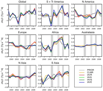
To examine the possible drivers of the interannual vari-ability in the N2O source, and to look at regional trends, the
fluxes were aggregated into eight different geographic and climatic regions and three ocean regions (see Figs. 7 and 8). Figure 7 shows the prior and posterior annual flux anomalies integrated over each land region. Generally, the results for all sensitivity tests were in close agreement with one another. The fact that the test using a flux climatology as the prior
0.0 0.2 0.4 0.6 0.8 1.0
0.0 0.2 0.4 0.6 0.8 1.0
Fig. 4. Annual mean (for 2003) error reduction (shown as a fraction
of 1) for the reference data set (upper panel) and the full data set (lower panel).
0.0 0.2 0.4 0.6 0.8
Fig. 5. Mean N2O flux (upper panel) and standard deviation (lower panel) for the period 1999–2009 shown for IAVA (units of g m−2a−1N).
(CLMR, orange) was close to the results using interannually varying prior fluxes provides confidence that the year-to-year variations are largely driven by the atmospheric observations. Furthermore, there is good agreement between the results from the tests using the reference vs. the full observation data set, indicating that a few sites are sufficient to capture flux in-terannual variability at (sub)-continental scales.
At the global scale, a weak positive trend in the N2O
source was found (0.05 Tg a−2N) but was not significant at the 95 % confidence level (p value of 0.5). The only statis-tically significant trend was found in South Asia, where the
−0.10 −0.05 0.00 0.05 0.10
Fig. 6. Mean N2O flux increments (a posteriori minus a pri-ori fluxes) for the period 1999–2009 shown for IAVA (units of g m−2a−1N).
source increased at a rate of 0.045 Tg a−2N (median of all sensitivity tests, p value of 0.006) between 1999 and 2009 (see Fig. 7). Although a similar trend (0.049 Tg a−2N) is seen in the prior fluxes, this signal is not only driven by the prior, as the test CLMR also shows a similar trend.
4 Discussion
4.1 Emission trends in South Asia
The economies of South Asia, in particular those of China and India, have undergone rapid growth in the past decade. This has been seen in increased industrialization and energy consumption. It has also led to a growing demand for food and thus an expansion and intensification of agriculture.
According to the Food and Agricultural Organization of the United Nations (FAO) statistics, nitrogen fertilizer con-sumption in China has increased on average by 0.66 Tg a−1N between 2002 and 2010 (http://www.fao.org/corp/statistics/ en/). During the same period, the total harvested area for all crops increased by 51 Mha, leading to further increases in agricultural emissions. As a simple approximation, using a 1.25 % emission factor for direct agricultural emissions, as recommended by the IPCC (Mosier et al., 1998), would lead to an increase of 0.008 Tg a−2N. These calculations do not account for indirect N2O emissions associated with
nitro-gen leaching and atmospheric transport of reactive nitronitro-gen, which lead to increased N2O emissions in areas distant from
where the fertilizer was applied. A more complete estimate of the increase in agricultural emissions, which also includes indirect emissions, is given by the EDGAR-4.2 inventory: on average 0.026 Tg a−2N between 2000 and 2008. Increased energy consumption in China has also led to greater N2O
emission, contributing 0.009 Tg a−2N and emissions from chemical production and solvent use contributing a further 0.002 Tg a−2N (EDGAR-4.2). In total (i.e. across all
sec-2000 2002 2004 2006 2008 −2 −1 0 1 2 Δ N2 O [Tg a − 1 N] Global 2000 2002 2004 2006 2008 −0.6 −0.4 −0.2 0.0 0.2 0.4 0.6 S + Tr America 2000 2002 2004 2006 2008 −0.6 −0.4 −0.2 0.0 0.2 0.4 0.6 N America 2000 2002 2004 2006 2008 −0.6 −0.4 −0.2 0.0 0.2 0.4 0.6 Δ N2 O [Tg a − 1 N] Europe 2000 2002 2004 2006 2008 −0.6 −0.4 −0.2 0.0 0.2 0.4 0.6 Africa 2000 2002 2004 2006 2008 −0.6 −0.4 −0.2 0.0 0.2 0.4 0.6 Australasia 2000 2002 2004 2006 2008 −0.6 −0.4 −0.2 0.0 0.2 0.4 0.6 Δ N2 O [Tg a − 1 N] N Asia 2000 2002 2004 2006 2008 −0.6 −0.4 −0.2 0.0 0.2 0.4 0.6 S Asia PRIOR CLMR IAVR IAVA IAVS IAVE
Fig. 7. Global and land regions annual flux anomalies (units
of Tg a−1N). The grey-shaded areas indicate El Niño events
(MEI ≥ 0.6).
tors), EDGAR-4.2 estimates that Chinese N2O emissions
have been increasing at an average rate of 0.042 Tg a−2N (from 2000 to 2008).
In India, a similar trend in nitrogen fertilizer consump-tion is seen with an average increase of 0.68 Tg a−1N from 2002 to 2010 (FAO). In contrast to China, however, there has been negligible change in crop area. Furthermore, despite the strong increase in nitrogen fertilizer use, EDGAR-4.2 does not estimate a large change in agricultural emissions of N2O
(only 0.005 Tg a−2N), nor does it in the total emissions (only 0.0075 Tg a−2N), for 2000 to 2008. It is beyond the scope of this study to speculate as to why there is an apparent dis-crepancy between the FAO statistics and the EDGAR-4.2 es-timate for agricultural emissions. However, it is noteworthy that the average change in total emissions for China and India (approximately 0.05 Tg a−2N) is in close agreement to that found for South Asia by the inversions (0.045 Tg a−2N). 4.2 Interannual variability in fluxes
4.2.1 Tropical and subtropical land
The largest interannual variations in N2O emissions are
seen in the tropical and subtropical land regions, i.e. trop-ical South America and South America, and Africa. In Fig. 7, periods with a multivariate ENSO index (MEI, http: //www.esrl.noaa.gov/psd/enso/mei/) value above 0.6, i.e. El Niño events, have been shaded in grey. El Niño events oc-curred from mid-2002 to 2003 and in 2007, with weak El Niño conditions between 2004 and 2006. The El Niño events of 2002 and 2007 coincide with negative N2O flux
2000 2002 2004 2006 2008 −0.6 −0.4 −0.2 0.0 0.2 0.4 0.6 Δ N2 O [Tg a − 1 N] Ocean 20N−90N 2000 2002 2004 2006 2008 −0.6 −0.4 −0.2 0.0 0.2 0.4 0.6 Ocean 20S−20N 2000 2002 2004 2006 2008 −0.6 −0.4 −0.2 0.0 0.2 0.4 0.6 Ocean 90S−20S
Fig. 8. Ocean region flux anomalies (units of Tg a−1N). The grey-shaded areas indicate El Niño events (MEI ≥ 0.6). (Legend the same as in Fig. 7.)
with positive N2O flux anomalies. (Unfortunately, there
are insufficient accurate N2O measurements available prior
to the late 1990s to resolve regional fluxes; hence, it is not possible to study the period of the strong El Niño of 1997– 1998.) Since our atmospheric transport model is nudged to ERA-interim wind fields (see Sect. 2.2), the effects of inter-annual variations in transport are accounted for. Therefore, it is unlikely that the correlation of the emissions with MEI is an artefact of ENSO-related atmospheric transport changes.
ENSO has a well-known climate impact in tropical and subtropical South America, Asia, Australia and southern Africa (Trenberth et al., 1998, and references therein) and may be driving the changes in N2O land flux, as proposed by
Thompson et al. (2013), Ishijima et al. (2009) and Saikawa et al. (2013). The strongest climate effects generally occur from December to February, and during an El Niño event these bring warm and dry conditions to the central and eastern parts of South America, southern Africa and tropical and subtropi-cal Asia. La Niña, on the other hand, is associated with cooler and wetter conditions in these regions. To investigate a pos-sible link between climate and N2O flux, we analysed
pre-cipitation, soil moisture and temperature data from ECMWF ERA-Interim (Dee et al., 2011) at 80 km resolution. These meteorological parameters are known to strongly influence the rates of denitrification and nitrification and to modulate N2O flux at the local scale (Davidson, 1993; Smith et al.,
1998). It is, however, beyond this scope of this study to fully analyse the sensitivity of N2O emissions to climate, which in
itself is an ambitious, albeit important, research topic. In this study, we only discuss correlations between meteorological anomalies and N2O fluxes and their possible causes.
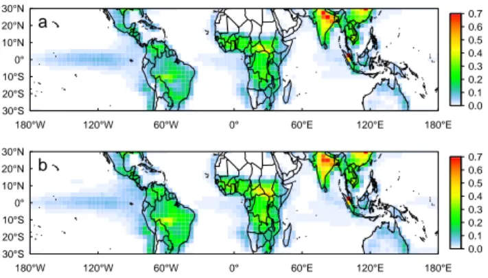
The strong negative N2O flux anomaly in 2002
corre-sponds with negative precipitation and soil moisture anoma-lies over tropical and subtropical South America and Africa (see Fig. 10), in areas with significant mean N2O flux (i.e. in
areas with a mean soil N2O flux above 0.1 g m−2a−1N
ac-cording to the prior flux estimate). Differences in N2O soil
fluxes between, for example, the El Niño year 2002 and the near-neutral year 2003 can be seen over Brazil and central Africa, where the flux is lower in 2002 (Fig. 9).
However, not all negative precipitation and soil moisture anomalies are associated with low N2O flux and vice versa.
The severity of the water deficiency may be important in
180°W 120°W 60°W 0° 60°E 120°E 180°E 30°S 20°S 10°S 0° 10°N 20°N 30°N b 0.0 0.1 0.2 0.3 0.4 0.5 0.6 0.7 180°W 120°W 60°W 0° 60°E 120°E 180°E 30°S 20°S 10°S 0° 10°N 20°N 30°N a 0.0 0.1 0.2 0.3 0.4 0.5 0.6 0.7
Fig. 9. Annual mean N2O flux (g m−2a−1N) from the inversion IAVA, shown for the tropics in the El Niño year 2002 (a) and the near-neutral year 2003 (b).
determining whether or not N2O production in soils is
af-fected. N2O flux peaks in soils with between 50 and 80 %
or 60 and 90 % water-filled pore space (WFPS), depending on soil type, and drops off exponentially below this thresh-old (Bouwman, 1998). Therefore, the water limitation would need to be severe enough to make a significant change in WFPS. A severe drought could potentially also affect the availability of reactive nitrogen in unfertilized regions by slowing the rate of mineralization of organic matter in soils (Borken and Matzner, 2009). An important link between soil moisture, mineralization rates and N2O flux in
tropi-cal soils on seasonal timestropi-cales has already been proposed by Potter et al. (1996), and may also be important on in-terannual timescales. Furthermore, using a data-calibrated biogeochemical model, Werner et al. (2007) found signif-icant interannual variability in the tropical rainforest soil N2O source, which was largely driven by changes in
rain-fall. For example, for African rainforests the N2O source was
found to change by 0.21 Tg a−1N (50 %) from 1993 to 1994 (Werner et al., 2007), a magnitude commensurate with the standard deviation of emissions from Africa in the inversions (0.3 Tg a−1N). In tropical and subtropical South America, the standard deviation of the emissions from the inversions is close to that for Africa (0.26 Tg a−1N), and represents about
10 % of the total mean flux of this region. 4.2.2 Temperate land
Interannual variations in temperate N2O soil fluxes, i.e. in
North America, North Asia and Europe, are smaller than those found in the tropics. In North America, low N2O flux
is found for 2005–2006 and coincides with negative precip-itation and soil moisture anomalies in the ECMWF ERA-Interim data (Dee et al., 2011) (see Fig. 10). In 2007, higher N2O fluxes are found and coincide with the return of
precip-itation rates to average values. High fluxes are also seen in 1999, and coincide with a positive soil temperature anomaly and a weak positive anomaly in soil moisture. In Europe, low
−0.5 0.0 0.5 Δ N2 O [Tg a − 1 N] N America −2 −1 0 1 2 T [K] −0.4 −0.2 0.0 0.2 0.4 Precip [m] 2000 2002 2004 2006 2008 2010 −0.02 −0.01 0.00 0.01 0.02 SWV [m 3/m 3] S + Tr America 2000 2002 2004 2006 2008 2010 Africa 2000 2002 2004 2006 2008 2010 Europe 2000 2002 2004 2006 2008 2010 S Asia 2000 2002 2004 2006 2008 2010
Fig. 10. Comparisons of the interannual variability in N2O flux with anomalies in soil temperature (T ), precipitation (Precip) and soil water volume (SWV) (ECMWF ERA-Interim). For the fluxes, the legend is the same as in Fig. 7. For the meteorological variables, the grey bars indicate the monthly anomaly and the solid line the interannual variability.
N2O flux is seen in 2005 and corresponds to a small negative
anomaly in temperature, soil moisture and precipitation (see Fig. 10). Although significant negative anomalies in precipi-tation and soil moisture also occurred in 2003, no anomaly was seen in the annual total flux for this year. However, the flux interannual variability (calculated from the monthly fluxes using a Butterworth filter to remove seasonal varia-tions) shows a negative flux anomaly of about 0.2 Tg a−1N in the second half of 2003 and a positive anomaly of similar magnitude in the first half of the year, which cancel out in the annual total.
4.2.3 Ocean
Considerable interannual variability in N2O flux is also seen
in the tropical (20◦N to 20◦S) and southern oceans (20◦S to 90◦S) (Fig. 8). In general, low N2O flux coincides with El
Niño, in 2002 and 2007, and high N2O flux with La Niña, in
2000, 2006 and 2008. The inversion results are fairly consis-tent for all sensitivity tests. One notable exception is in the year 2006, where in the tropical ocean the inversion CLMR (using a climatological prior) stands out with a strong pos-itive anomaly, which is not seen in the other inversions for which the interannually varying prior was used. This discrep-ancy may be a result of too few degrees of freedom for the flux to depart from the prior N2O flux estimate, which is too
low in the interannually varying fluxes.
ENSO has a strong influence on ocean upwelling and thus on air–sea gas exchange. During El Niño, warm water in the western Pacific migrates eastward and reduces upwelling in the eastern Pacific off the coast of South America, while dur-ing La Niña the process is reversed and there is an increase in upwelling (McPhaden et al., 2006). Changes in upwelling
af-fect air–sea N2O fluxes through physical and biological
pro-cesses: physically, by changing the supply of N2O-rich water
from below the euphotic zone to the surface and thereby the partial pressure of N2O in the surface water, and biologically,
by changing the supply of nutrients to the surface layer and thus primary production and the production of N2O within
the surface layer (Nevison et al., 2007). These processes are parameterized in the biogeochemistry model PISCES, used for the prior ocean N2O flux in the inversion (Dutreuil et al.,
2009). PISCES was coupled to a climate model and is thus sensitive to ENSO driven changes. However, as the climate model was unconstrained, the variability does not necessarily reflect the real timing of ENSO. The atmospheric inversion helps constrain the timing of the ENSO driven changes in ocean N2O flux and verifies the magnitude of these changes,
which are of the order of 0.4 Tg a−1N globally.
5 Summary and conclusions
We present estimates of N2O fluxes from 1999 to 2009 based
on the inversion of atmospheric transport and observations of atmospheric N2O mole fractions. To determine the
sensitiv-ity of the inversion results to the coverage of the observa-tions, the prior fluxes used, the strength of the stratospheric sink and the assigned observation error, five different inver-sion tests were carried out. All five inverinver-sions produced con-sistent results within the posterior error margin, which indi-cates a fair representation of the prior errors in the inversion system. Over the 11 years period, the global total N2O source
varied from 17.5 to 20.1 Tg a−1N (control inversion, IAVA), with a SD of 0.77 Tg a−1N. The year-to-year variability in the global source was significantly larger than the variability