Positron range in PET imaging: an alternative approach for assessing and correcting the blurring

HAL Id: cea-02134410

https://hal-cea.archives-ouvertes.fr/cea-02134410

HAL is a multi-disciplinary open access archive for the deposit and dissemination of sci-entific research documents, whether they are pub-lished or not. The documents may come from teaching and research institutions in France or abroad, or from public or private research centers.

L’archive ouverte pluridisciplinaire HAL, est destinée au dépôt et à la diffusion de documents scientifiques de niveau recherche, publiés ou non, émanant des établissements d’enseignement et de recherche français ou étrangers, des laboratoires publics ou privés.

Positron range in PET imaging: an alternative approach

for assessing and correcting the blurring

L Jødal, C. Le Loirec, C. Champion

To cite this version:

L Jødal, C. Le Loirec, C. Champion. Positron range in PET imaging: an alternative approach for assessing and correcting the blurring. Physics in Medicine and Biology, IOP Publishing, 2012, 57 (12), pp.3931-3943. �10.1088/0031-9155/57/12/3931�. �cea-02134410�

Positron range in PET imaging: an alternative approach for

assessing and correcting the blurring

Running head: Positron range in PET imaging

Authors

L Jødal1_{, C Le Loirec}2 _{and C Champion}3

1 _{Department of Nuclear Medicine, Aalborg University Hospital, Denmark}

2 _{Laboratoire Modélisation, Simulation et Systèmes, DRT/LIST/DCSI/LM2S, CEA Saclay, Gif-sur-Yvette,}

France

3 _{Laboratoire de Physique Moléculaire et des Collisions, Université Paul Verlaine-Metz, France}

Abstract

Background: Positron range impairs resolution in PET imaging, especially for high-energy emitters

and for small-animal PET. De-blurring in image reconstruction is possible if the blurring distribution is known. Further, the percentage of annihilation events within a given distance from the point of positron emission is relevant for assessing statistical noise.

Aims: The paper aims to determine positron range distribution relevant for blurring for seven

medically relevant PET isotopes, 18_F, 11_C, 13_N, 15_O, 68_Ga, 62_{Cu, and} 82_{Rb, and derive empirical}

formulas for the distributions. The paper focuses on allowed-decay isotopes.

Methods: It is argued that blurring at the detection level should not be described by positron range r,

but instead the 2D-projected distance δ (equal to the closest distance between decay and line-of-response). To determine these 2D distributions, results from a dedicated positron track-structure Monte Carlo code, EPOTRAN, were used. Other materials than water were studied with PENELOPE.

Results: The radial cumulative probability distribution G2D(δ) and radial probability density

distribution g2D(δ) were determined. G2D(δ) could be approximated by the empirical function 1 –

positron energy in MeV and δ in mm. Radial density distribution g2D(δ) could be approximated by

differentiation of G2D(δ). Distributions in other media were very similar to water.

Conclusion: Positron range is important for improved resolution in PET imaging. Relevant

distributions for positron range have been derived for seven isotopes. Distributions for other allowed-decay isotopes may be estimated with the above formulas.

Keywords: Monte Carlo simulation, positron range, spatial resolution, annihilation, PET, point spread

function

PACS classification: 87.57.uk (Positron emission tomography)

Submitted to: Physics in Medicine and Biology

1. Introduction

Because of the improving spatial resolution of the physical detectors, the distance from positron emission to positron annihilation (positron range) is becoming a factor of increasing importance for the spatial resolution of positron emission tomography (PET). Positron range introduces uncertainty in the position of the positron emitter, resulting in blurring of the PET images. This effect is very clearly seen for high-energy emitters such as 82_{Rb, but also for less energetic emitters in small-animal PET imaging where blurring on a millimetre}

scale is important.

While positron range in itself is a fundamental physical aspect of the slowing-down processes leading to annihilation, it is possible to correct for the blurring in the reconstructed images, if the reconstruction algorithm incorporates knowledge of spatial distribution of the blurring effect (Cal-González et al 2009;Rahmim et al 2008;Ruangma et al 2006). Therefore, the distribution of positron ranges and its effect on PET imaging is a subject of prime importance, especially as technical advances may further improve detector resolution.

A point source emitting positrons will give rise to a three-dimensional (3D) distribution of annihilation points, which will characterize the positron range effect in the reconstructed images. But since a PET scanner measures lines of response (LORs), not annihilation positions, the 3D distribution is hard to measure directly (this also holds for Time-of-Flight PET, which reduces the length of the LOR, but still does not determine a point position). To determine positron range, Derenzo (1979) made a series of often-cited measurements using material of very low density, in an experimental set-up where only a narrow plane was measured at a time. This corresponds to projecting the 3D annihilation distribution onto a single line, giving the 1D representation often used in papers on positron range, see e.g. (Blanco 2006;Champion et al 2007;Levin et al 1999).

However, considering a single detector pair (rather than a full detector ring), the logical projection will be 2D: The detector pair measures in the plane orthogonal to the LOR defined by the two detectors, and positron range influences not only axial resolution (1D) but also transversal resolution. Thus, for a reconstruction algorithm modelling positron range at the level of LORs, the distribution of the 2D projection of annihilation points will be very relevant.

In any homogeneous medium and in absence of magnetic field, the situation is spherically symmetrical, and the mathematical information in the 3D, 1D, and 2D distributions will be the same, but converting e.g. a 1D distribution to a 2D distribution is not a simple calculation. However, 2D projections seem to have been given only little attention in the literature. Derenzo (1979) computed curves for 11_C, 68_Ga,

and 82_{Rb (from a} 82_{Sr source, which decays to} 82_{Rb by electron capture) showing the “Fraction projected}

annihilations occurring within a circle of radius R”, i.e., the cumulated 2D probability distribution. Sánchez-Crespo et al (2004) investigated 18_F, 15_{O, and} 82_{Rb by projecting the 3D distribution onto a plane and}

reported point spread functions of this projection along a line. And recently, Cal-González et al (2010;2011) have considered 2D representations of the annihilation distribution and compared them with other representations. But little other work seems to have been conducted on 2D representations of the annihilation distribution.

The present work aims to determine in details the cumulative 2D distributions for a series of medically relevant PET isotopes by means of a previously published dedicated positron track-structure Monte Carlo

simulation (Champion et al 2006;Champion et al 2007). Furthermore, it is aimed to provide a systematic procedure for estimating the cumulative distribution for other allowed-decay PET isotopes given only the mean positron energy Emean. (A beta decay is allowed if parity is unchanged and nuclear spin change is 0 or ±1 (Krane 1988); e.g. 1+ _{→ 0}+ _{as in the decay} 18_{F →} 18_{O.) The focus on allowed-decay PET isotopes is}

practical. The energy distributions can be described by known, analytical functions, and very many of the medical PET isotopes decay by allowed decay. Besides, differential distributions will be provided by following the same methodology. The results from the present Monte Carlo code (EPOTRAN) is compared with results from the more common PENELOPE code, and the influence of other biological media than water is estimated.

2. Material and methods

2.1 Geometry and notation

The complete blurring of a point source in an actual measurement will depend not only on positron range but also on photon non-collinearity and the properties of the detection system (such as crystal size and depth of interaction). However, all these effects can be considered individually and afterwards combined (Levin et al 1999;Qi et al 1998;Rahmim et al 2008). In the present context we will assume point-like detectors and 180° relative angle of the two photons emitted from annihilations, i.e., focus on positron range.

Consider a point source located at (0,0,0) in a Cartesian coordinate system. Assuming spherical symmetry, the volume density f(x,y,z) of annihilatons is function of range: f(x, y, z) = f(r). Following the notation of Cal-González et al (2010), we will define the radial density as g3D(r) = 4πr2 f(r) = 4πr2 f(x,y,z).

The LORs measured parallel to a given direction will be cylindrically symmetrically distributed. As the distribution of LORs will be the same for all directions, we can treat the situation as if all LORs were parallel to the same direction. Taking the z axis as the (arbitrary) choice of direction, the projection is onto

the xy plane. The distance from origin in 2D,

_δ

source and the LOR. Again we have symmetry: The 2D density distribution f(x,y) is a function of these distances, f(x, y) = f(δ), with radial density g2D(δ) = 2πδ f(δ).

The cumulative probability distribution G2D(δ), i.e. the probability that a LOR will have distance from the point source no greater than δ, can be calculated by integration:

.' ) ' ( ) ( 0 2 2 =

∫

Our notation for g2D and G2D is consistent with that of Cal-González et al (2010), except that we have chosen letter δ for 2D radius (LOR distances from point source), reserving r for 3D radius (positron range).

2.2 Positron energy spectra and Monte Carlo simulation

The following series of medically relevant PET isotopes were considered: 18_F, 11_C, 13_N, 15_O, 68_Ga, 62_{Cu, and} 82_{Rb. These are all allowed-decay isotopes whose energetic disintegration spectra are represented by}

(Venkataramaiah et al 1985) dE E E E p E Z F C dE E N( ) = ⋅ ( , )⋅ ⋅ ⋅( _max− ) , (2)

with E and Emax the energy and maximal energy of β particles, p the corresponding momentum and C a normalization constant. F(Z,E) represents the Fermi factor used for taking into account the effect of the Coulomb field on the electron distribution.

The 3D distributions f(x, y, z) of annihilation points were determined by using the full-differential Monte Carlo track-structure code, called EPOTRAN (an acronym for Electron and POsitron TRANsport in liquid and gaseous water) developed by Champion and Le Loirec to study the decay of positron emitters of medical interest (Champion et al 2007;Le Loirec et al 2007). In brief, for each isotope considered, a large number (about 250 000) positron tracks were simulated until annihilation, including all the processes, namely, ionization, excitation, elastic scattering, and positronium (Ps) formation. For more details, we refer the interested reader to (Champion et al 2012). The distribution g2D(δ) were determined by binning

2

2 _y

x + =

δ

2.3 Generalization of distributions

The resultant functions G2D(δ) were compared among isotopes in two ways, namely, either by plotting

G2D(δ) as a function of δ, or by plotting G2D(δ) as a function of δ/Rmean, where Rmean is the mean range of positrons for the isotope under consideration:

∫

∫∫∫

An empirical formula for G2D(δ) was then derived for each allowed-decay isotope, based on two adjustable parameters. The dependence of the parameters on mean positron energy Emean was also investigated. To estimate differential distributions g2D(δ), the empirical formula for G2D(δ) was differentiated, and the results compared with distributions of g2D(δ) determined from the Monte Carlo data.

2.4 Effects of variation in biological tissues

For a medium of a given composition, the range and thereby δ will scale inversely with density. But the shape of the positron range distribution may change with different composition, see e.g. (Lehnert et al 2011). Presently, EPOTRAN is not able to simulate positron track structure in a biological medium other than water. We have thus used the Monte Carlo code PENELOPE (2006 release) (Salvat et al 2006) first to compare density-scaled range of positrons in biologically relevant materials with the range in water and secondly to study the decay of 18_{F in water, lung and bone.}

PENELOPE is a Monte Carlo code of general purpose that permits us to simulate the coupled transport of photons, electrons and positrons in matter with a very good accuracy at low energies. Photons are transported within the conventional detailed method whereas electrons and positrons are simulated using a mixed scheme where interactions are classified into hard and soft. Hard events are simulated step by step and involve angular deflection or energy losses above user-defined cutoffs whereas soft events occurring between 2 hard collisions are simulated by means of an artificial single event. Simulation is controlled by seven parameters, fixed for the various materials used in the geometry:

(i) The absorption energies Eabs is the energy at which the track evolution is stopped. The kinetic energy of the particle is then locally deposited.

(ii) C1 is the average angular deflection between 2 hard elastic collisions.

(iii) C2 is the maximal fractional energy loss between 2 hard elastic collisions.

(iv) WCC is the cutoff energy for hard inelastic interactions.

(v) WCR is the cutoff energy for hard bremsstrahlung emission.

To be as close as possible as the simulations performed with EPOTRAN, we have chosen for water, lung and bone the same set of parameters which corresponds to a detailed simulation, thus Eabs = 100 keV for photons, electrons and positrons and C1, C2, WCC and WCR are equal to zero.

Tracking particles in PENELOPE is not obvious. It is however possible to determine the point of creation of particles, and in our case of annihilation photons. We have thus used a geometry consisting in concentric cylinders separated by 10 µm, which is the bin used for the distribution g2D(δ). The cylinders are centred on (0;0;0) which is the point of emission of positrons and they are full of water, bone or lung depending on the tissue under investigation. The simulation runs until the photons are detected on a spherical phase-space file (PSF) which stores a lot of information concerning the particles and especially the body (the cylinder in our case) where they have been created. Thanks to these data, we can thus determine directly the 2D distribution of annihilation points and obtain the cumulative probability G2D(δ).

3. Results

3.1 Ranges and cumulative probability distributions

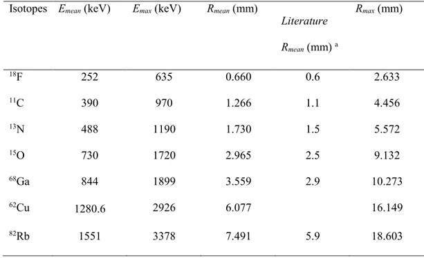
The investigated radio-isotopes are listed in Table 1 along with mean and maximum values for energy and range for the emitted positrons; for more details see (Champion et al 2007;Le Loirec et al 2007). Compared to other results from the literature (see Table 1 and figure 1) we obtain somewhat larger values for

Rmean. This difference is due to the inclusion of Ps formation in the simulation, as the electrically neutral Ps loses energy more slowly than the charged e+ _{particle (Champion 2003;Champion et al 2006).}

The literature results for Rmean do not include experimental data. Experimental results on Rmean are, unfortunately, scarce. Cho et al (1975) measured on a line source and determined an "effective range" from

the FW(0.1)M on this distribution, and Derenzo (1979;1986) determined the root-mean-square (rms) spread for the 1D distribution. While such data can be used as indicators for Rmean, we are not aware of experimental results that aim at determining Rmean as such.

It should be mentioned that while the Monte Carlo code used here assumes the neutral Positronium (Ps) to lose its kinetic energy mainly through phonon interactions at all energies, recent experimental results (Brawley et al 2010a;Brawley et al 2010b) found unexpectedly large Ps interactions at sub-keV energies. While these results are in themselves very interesting, a discrepancy in Ps cross section at very low energy will only have marginal influence on our results, since most of the path travelled by Ps will be with much higher kinetic energy.

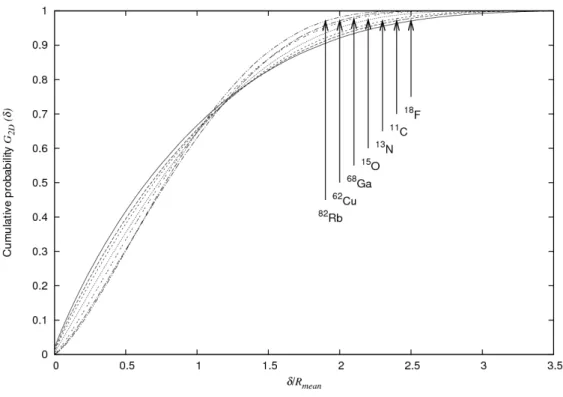
The calculated cumulative probabilities G2D(δ) for closest distance δ are shown in figure 2. Not surprisingly, the distance δ that includes a given fraction of the LORs, depends on the energy spectrum of the emitted positrons. However, when the same data are plotted as a function of δ/Rmean, i.e. scaled by the

isotope-dependent mean range, the results are rather similar among isotopes (see figure 3).

Table 1: Mean and maximum values for energy and range for the emitted positrons (Champion et al 2007;Le Loirec et al 2007).

Isotopes Emean (keV) Emax (keV) Rmean (mm)

Literature Rmean (mm) a Rmax (mm) 18_{F 252 635 0.660 0.6 2.633} 11_{C 390 970 1.266 1.1 4.456} 13_{N 488 1190 1.730 1.5 5.572} 15_{O 730 1720 2.965 2.5 9.132} 68_{Ga 844 1899 3.559 2.9 10.273} 62_{Cu 1280.6 2926 6.077 16.149} 82_{Rb 1551 3378 7.491 5.9 18.603} a _{(Partridge et al 2006)}

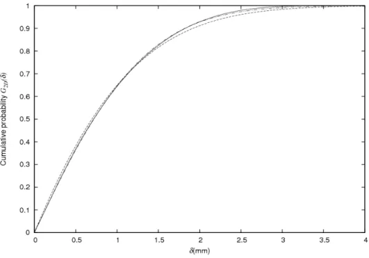
Figure 1: Cumulative probabilities for 18_{F obtained with EPOTRAN and PENELOPE.}

Figure 3: Cumulative probabilities G2D(δ) versus δ/Rmean.

3.2 Empirical estimation of cumulative probability distributions

Despite their similarity, the plots in figure 3 cannot be described by a single curve. Instead we have for each isotope fitted the cumulative probability curves reported in figure 2 by the following empirical function:

). exp( 1 ) (

_δ

_δ

_δ

ζ

This form is chosen such that for any positive values of A and B, it will correctly rise monotonously from ζ(0) = 0 towards 1, ζ(∞) = 1. Furthermore, for any probability 0 ≤ ζ < 1 considered, the corresponding value of δ can be found as the positive solution to the equation

. 0 ) 1 ln( 2 ₊

_δ

_ζ

δ

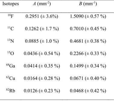
Table 2: Fitting parameters for the empirical cumulative probability given by (4). The standard errors are indicated into brackets for each isotope.

Isotopes A (mm-2_{) B (mm}-1₎ 18_{F 0.2951 (± 3.6%) 1.5090 (± 0.57 %)} 11_{C 0.1262 (± 1.7 %) 0.7010 (± 0.45 %)} 13_{N 0.0885 (± 1.0 %) 0.4681 (± 0.38 %)} 15_{O 0.0436 (± 0.54 %) 0.2266 (± 0.33 %)} 68_{Ga 0.0414 (± 0.35 %) 0.1499 (± 0.34 %)} 62_{Cu 0.0164 (± 0.28 %) 0.0671 (± 0.40 %)} 82_{Rb 0.0126 (± 0.23 %) 0.0468 (± 0.42 %)}

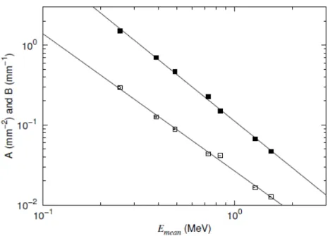
The parameters A and B obviously depend on isotope. In figure 3 we scaled the curves by the isotope-dependent Rmean. For the parameters A and B we investigated instead dependence of the more easily determined value Emean and found that they could be described as power functions of Emean:

A = 0.0266·(Emean)-1.716 and B = 0.1119·(Emean)-1.934, (6)

where Emean is given in MeV, and the units of A and B are mm-2 and mm-1, respectively. The variations of A and B with Emean as well as the interpolated power functions are reported in figure 4.

Figure 4: The fitting parameters A and B (open and solid squares, respectively) versus the mean energy of the isotope under consideration.

As a simple check of these expressions, we study also the case of 52_{Fe, a radio-metal}

generator-produced isotope which emits positrons of relatively low energy, Emax = 803.6 keV and Emean = 344 keV = 0.344 MeV. Clinically, 52_{Fe has been used in haematological studies to follow iron kinetics, but such studies}

are complicated by the fact that 52_{Fe decays to another PET isotope,} 52m_{Mn (Haddad et al 2008;Lubberink et} al 1999). By using (6), we have estimated the fitting parameters as A = 0.1660 mm-2 _{and B = 0.8813 mm}-1_.

Figure 5 shows the calculated G2D(δ) for 52Fe along with the empirical function ζ(δ) described by these values of A and B.

Figure 5: Calculated function G2D(δ) along with empirical function ζ(δ) from estimated values of A and B for 52_{Fe (solid and dashed line, respectively). A direct fit to the data is shown as a dot-dash-dot line almost}

coinciding with the full line.

3.3 Radial probability density distributions

For determination of point spread functions (PSFs), the probability density distribution should be known, either as area density, f(x, y) = f(δ), or as radial density, g2D(δ). We here focus on the radial probability density, which can be compared to the result of differentiation of the estimate for cumulated probability, ζ(δ) from (4): ). exp( ) 2 ( ) ( 2 2 2

_δ

δ

δ

δ

ζ

δ

δ

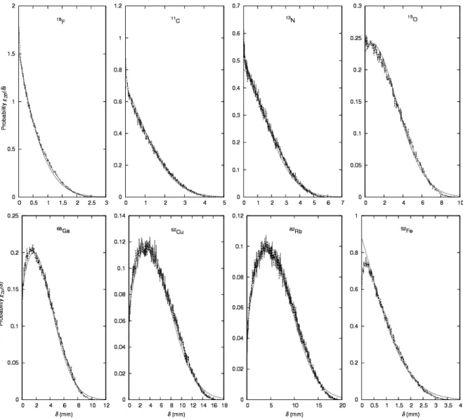
It will be noted that dζ/dδ is normalized to total area 1, since ζ(0) = 0 and ζ(∞) = 1. The Monte Carlo data are compared with the result of (7) in figure 6.

Figure 6: Functions g2D(δ) taken from Monte Carlo calculations (broken lines) compared with the expression from (7) (smooth lines), using values of A and B from table 2. For 52_{Fe, the values of A and B}

from (6) were used. Monte Carlo data are reported with a 10 µm bin for 18_F, 11_C, 13_{N, and} 52_{Fe, and with a 30}

µm bin for 15_O, 68_Ga, 62_{Cu, and} 82_Rb.

3.4 Effects of variation in biological tissues

The PENELOPE results for density-scaled positron range in different media are given in Table 3. It is seen that soft tissue has only very small differences from water, while bone tissue deviates by about 13%.

Table 3: Approximate mean range for two isotopes (chosen to represent low and high energy) calculated with PENELOPE in the continuing slowing down approximation (CSDA). For soft and lung tissue, the largest difference from water is 1.2% whereas it is up to 13% for bone tissue.

Biological materials (ICRP compositions) range · density (g·cm-2₎

Name Density ρ (g·cm-3₎ 18_F 62_Cu Water 1.00 0.0622 0.595 Lung 0.26 0.0634 0.597 Adipose 0.98 0.0613 0.591 Muscle 1.07 0.0635 0.602 Bone 1.92 0.0702 0.666

In figure 7, we have reported the cumulative 2D probabilities obtained in PENELOPE for 18_{F in water,}

bone and lung. The data are plotted as a function of δ·ρ with ρ the density of the biological tissue. The tendency for bone-data to have larger distances can be seen as the bone curve being slightly below the other two curves in the upper half of the figure, but overall the density-corrected distributions are very similar for all three media.

Figure 7: Cumulative probability for water (solid line), bone (dash line) and lung (dotted line) as a function of δ · ρ. All three curves are based on PENELOPE results.

4. Discussion

4.1 Cumulative and differential 2D probability distributions

As noted in the introduction, the choice of 2D distributions is very relevant when considering measurements by individual detector pairs. The cumulative distribution G2D(δ) shows us that for all the investigated isotopes, almost 2/3 of the annihilations take place within δ ≤ Rmean (see figure 3), meaning that Rmean can be used as rough estimate of the expected broadening due to positron range.

When based on Monte Carlo data, rather than mathematical functions, the cumulative (integral) distribution is more robust than the differential distribution. But a reconstruction algorithm involving modelling of positron range will typically need the differential distribution, either as area density f(δ) or radial density g2D(δ). As demonstrated in figure 6, the radial distributions can be well approximated by use of (7) with the values of A and B from Table 2. If A and B are determined from the simple, empirical relations (6) then the distribution will of course be less precise, but the curves for 52_{Fe in Figures 5 and 6 indicates that}

such distributions can be used as a first approximation for other allowed-decay isotopes than those in Table 2.

Our focus on radial density has the advantage of avoiding the very peaked (cusp-shaped) distributions found for both 1D (Derenzo 1979) and 2D (Sánchez-Crespo et al 2004) non-radial distributions. These peaks are so sharp that the peak height becomes dependent on the details of the calculations (e.g., bin size), meaning that measures dependent on peak height (such as FWHM) do not have a strict meaning (Levin et al 1999).

In fact, our own results indicate that the radial distribution g2D(δ) do not necessarily go to zero for δ → 0 (see figure 6), i.e. the area distribution f(δ) = g2D(δ) / (2πδ) may diverge for δ → 0, in which case FWHM is meaningless. Note that such a divergence is not unphysical as long as the area under the singularity is finite. For example, a simple harmonic oscillator, x = A sin(ωt), will have a density distribution for x which

diverges at x = ±A, because velocity is zero in these positions. In our case, g2D can be integrated into G2D, with the (physically correct) implication that only a finite number of positrons will be detected near δ = 0.

It can be argued against the form (4) for the cumulative distribution G2D(δ)estimate = ζ(δ) that it never

reaches 1, and therefore the differential distributions g2D(δ)estimate = dζ/dδ never fall to 0, despite positrons

having a maximum range. The effect of this can be seen on figure 6, where the final part of the curves

g2D(δ)estimate tend to be slightly above the Monte Carlo data, especially for the high-energy isotopes. Similar

objections could however be raised against describing positron range distributions by exponentials (Derenzo 1979) or Gaussian functions (Palmer et al 1992). Mathematically, it can be seen that dζ/dδ will eventually approach the zero value faster than a Gaussian function: dζ/dδ can be considered the product of a Gaussian, exp(-Aδ2_{), and a factor that goes towards zero for large distances, (2Aδ + B)·exp(-Bδ), possibly after an}

initial rise. If a cut-off distance δcut-off is introduced, setting g2D(δ)estimate = 0 for δ > δcut-off, then the area under the curve will then be slightly less than 1, namely ζ(δcut-off). A possible choice for δcut-off can be Rmax which can be estimated from Emean as a linear function, based on Table 1 (fit not shown).

In short, our formulation based on A and B is suitable for applications dependent on the whole distribution (such a de-blurring), while it is less suitable or unsuitable for applications sensitive to the behaviour of a small fraction of the positrons (such as the determination of maximal distances). Figure 7 indicates that the same values of A and B can be used for different media if distances are scaled by density, as it has already been proposed by Lehnert et al (2011) for a 1D distribution model.

4.2 Limitations

The current study was made only for allowed-decay isotopes. Non-allowed-decay isotopes can have other relations between Emean and spectrum shape, meaning that the empirical relation (6) cannot be expected to give usable results for non-allowed-decay isotopes. As an example we tried it for 124_{I (data not shown),}

which is non-allowed-decay, and found large discrepancies from expected G2D(δ).

Nowadays, it is well-known that when high-energy positron emitters are used in PET scanning, the positron range adds to resolution degradation. In the major part of existing studies this degradation is related to the positron range (r). In the present work, we have proposed to use not the positron range but instead the shortest distance (δ) between point of emission and the LOR. Annihilation point radial 2D density distributions as well as cumulated probabilities for a series of medically relevant PET isotopes were provided by means of Monte Carlo simulation. Empirical expressions of these distributions were then proposed for the allowed-decay PET isotopes here investigated.

These results allow easy estimation of the percentage of annihilations happening within a given distance and may give approximate density distributions for use in reconstruction algorithms taking positron range into account.

Conflicts of interest: none

References

Blanco A. 2006 Positron Range Effects on the Spatial Resolution of RPC-PET. 2006 IEEE

Nucl.Sci.Symp.Conf.Rec. 2570-2573.

Brawley SJ, Armitage, S, Beale, J, Leslie, DE, Williams, AI, and Laricchia, G. 2010a Electron-Like Scattering of Positronium. Science 330 789.

Brawley SJ, Williams, AI, Shipman, M, and Laricchia, G. 2010b Resonant Scattering of Positronium in Collision with CO2. Phys.Rev.Lett. 105 263401.

Cal-González J, Herraiz, JL, Corzo, PMG, and Udías, JM. 2011 A General Framework to study Positron Range Distributions. 2011 IEEE Nuclear Science Symposium Conference Record 2733-2737.

Cal-González J, Herraiz, JL, Espana, S, Desco, M, Vaquero, JJ, and Udias, JM. 2009 Positron Range Effects in High Resolution 3D PET Imaging. 2009 IEEE Nuclear Science Symposium Conference Record 2788-2791.

Cal-González J, Herraiz, JL, España, S, Desco, M, Vaquero, JJ, and Udías, JM. 2010 Validation of PeneloPET Positron Range Estimations. 2010 IEEE Nucl.Sci.Symp.Conf.Rec. 2396-2399.

Champion C. 2003 Theoretical cross sections for electron collisions in water: structure of electron tracks.

Phys.Med.Biol. 48 2147-2168.

Champion C and Le Loirec, C. 2006 Positron follow-up in liquid water: I. A new Monte Carlo track-structure code. Phys.Med.Biol. 51 1707-1723.

Champion C and Le Loirec, C. 2007 Positron follow-up in liquid water: II. Spatial and energetic study for the most important radioisotopes used in PET. Phys.Med.Biol. 52 6605-6625.

Champion C, Le, LC, and Stosic, B. 2012 EPOTRAN: a full-differential Monte Carlo code for electron and positron transport in liquid and gaseous water. Int.J Radiat.Biol. 88 54-61.

Cho ZH, Chan, JK, Ericksson, L, Singh, M, Graham, S, MacDonald, NS, and Yano, Y. 1975 Positron ranges obtained from biomedically important positron-emitting radionuclides. J Nucl Med 16 1174-1176.

Derenzo, SE 1979 Precision measurement of annihilation point spread distributions for medically important positron emitters, in Positron Annihilation, Hasiguti RR and Fuliwara K, eds., (The Japan Institute of Metals, Sendai, Japan), pp. 819-823.

Derenzo SE. 1986 Mathematical Removal of Positron Range Blurring in High-Resolution Tomography.

IEEE Trans.Nucl.Sci. 33 565-569.

Haddad F, Ferrer, L, Guertin, A, Carlier, T, Michel, N, Barbet, J, and Chatal, JF. 2008 ARRONAX, a high-energy and high-intensity cyclotron for nuclear medicine. Eur.J.Nucl.Med.Mol.Imaging 35 1377-1387. Krane, KS 1988, Introductory nuclear physics, 2nd edn, John Wiley & Sons.

Le Loirec C and Champion, C. 2007 Track structure simulation for positron emitters of medical interest. Part I: The case of the allowed decay isotopes. Nucl.Instrum.Methods Phys.Res., Sect.A 582 644-653.

Lehnert W, Gregoire, MC, Reilhac, A, and Meikle, SR. 2011 Analytical positron range modelling in heterogeneous media for PET Monte Carlo simulation. Phys.Med.Biol. 56 3313-3335.

Levin CS and Hoffman, EJ. 1999 Calculation of positron range and its effect on the fundamental limit of positron emission tomography system spatial resolution. Phys.Med.Biol. 44 781-799.

Lubberink M, Tolmachev, V, Beshara, S, and Lundqvist, H. 1999 Quantification aspects of patient studies with Fe-52 in positron emission tomography. Appl.Radiat.Isot. 51 707-715.

Palmer MR and Brownell, GL. 1992 Annihilation density distribution calculations for medically important positron emitters. IEEE Trans.Med.Imaging 11 373-378.

Partridge M, Spinelli, A, Ryder, W, and Hindorf, C. 2006 The effect of β+ _{energy on performance of a small}

animal PET camera. Nucl.Instrum.Methods Phys.Res., Sect.A 568 933-936.

Qi JY, Leahy, RM, Cherry, SR, Chatziioannou, A, and Farquhar, TH. 1998 High-resolution 3D Bayesian image reconstruction using the microPET small-animal scanner. Phys.Med.Biol. 43 1001-1013.

Rahmim A, Tang, J, Lodge, MA, Lashkari, S, Ay, MR, Lautamaki, R, Tsui, BMW, and Bengel, FM. 2008 Analytic system matrix resolution modeling in PET: an application to Rb-82 cardiac imaging.

Phys.Med.Biol. 53 5947-5965.

Ruangma A, Bai, B, Lewis, JS, Sun, XK, Welch, MJ, Leahy, R, and Laforest, R. 2006 Three-dimensional maximum a posteriori (MAP) imaging with radiopharmaceuticals labeled with three Cu radionuclides.

Nucl.Med.Biol. 33 217-226.

Salvat F, Fernández-Varea JM, and Sempau J 2006 PENELOPE—A code system for Monte Carlo simulation of electron and photon transport OECD Nuclear Energy Agency Issy-les-Moulineaux, France

Sánchez-Crespo A, Andreo, P, and Larsson, SA. 2004 Positron flight in human tissues and its influence on PET image spatial resolution. Eur.J.Nucl.Med.Mol.Imaging 31 44-51.

Venkataramaiah P, Gopala, K, Basavaraju, A, Suryanarayana, SS, and Sanjeeviah, H. 1985 A Simple Relation for the Fermi Function. J.Phys.G: Nucl.Part.Phys. 11 359-364.