HAL Id: halshs-01813382
https://halshs.archives-ouvertes.fr/halshs-01813382
Submitted on 13 Jun 2018
HAL is a multi-disciplinary open access
archive for the deposit and dissemination of
sci-entific research documents, whether they are
pub-lished or not. The documents may come from
L’archive ouverte pluridisciplinaire HAL, est
destinée au dépôt et à la diffusion de documents
scientifiques de niveau recherche, publiés ou non,
émanant des établissements d’enseignement et de
Human mobility: Models and applications
Hugo Barbosa, Marc Barthelemy, Gourab Ghoshal, Charlotte James, Maxime
Lenormand, Thomas Louail, Ronaldo Menezes, José Ramasco, Filippo Simini,
Marcello Tomasini
To cite this version:
Hugo Barbosa, Marc Barthelemy, Gourab Ghoshal, Charlotte James, Maxime Lenormand, et al..
Human mobility: Models and applications. Physics Reports, Elsevier, 2018, 734 (734), pp.1-74.
�10.1016/j.physrep.2018.01.001�. �halshs-01813382�
Human Mobility: Models and Applications
Hugo Barbosa-Filhoa, Marc Barthelemyb,c, Gourab Ghoshala,∗, Charlotte R. Jamesd, Maxime Lenormande, Thomas Louailg, Ronaldo Menezesh,∗, Jos´e J. Ramascof,
Filippo Siminid, Marcello Tomasinih
aDepartment of Physics& Astronomy and Goergen Institute of Data Science, University of Rochester,
Rochester, NY, USA
bInstitut de Physique Th´eorique, CEA, CNRS-URA 2306, F-91191, Gif-sur-Yvette, France cCentre d’Etudes et de Math´ematique Sociales, EHESS, Paris 75006, France
dDepartment of Engineering Mathematics, University of Bristol, UK eIrstea, UMR TETIS, 500 rue JF Breton, 34093 Montpellier, France
fInstituto de F´ısica Interdisciplinar y Sistemas Complejos IFISC (CSIC-UIB), Campus UIB, 07122 Palma
de Mallorca, Spain
gCNRS, UMR 8504 G´eographie-cit´es, 13 rue du four, F-75006 Paris, France hBioComplex Laboratory, School of Computing, Florida Institute of Technology, Melbourne, USA
Abstract
Recent years have witnessed an explosion of extensive geolocated datasets related to human movement, enabling scientists to quantitatively study individual and collective mobility patterns, and to generate models that can capture and reproduce the spatiotem-poral structures and regularities in human trajectories. The study of human mobility is especially important for applications such as estimating migratory flows, traffic fore-casting, urban planning, and epidemic modeling. In this survey, we review the ap-proaches developed to reproduce various mobility patterns, with the main focus on recent developments. This review can be used both as an introduction to the funda-mental modeling principles of human mobility, and as a collection of technical meth-ods applicable to specific mobility-related problems. The review organizes the subject by differentiating between individual and population mobility and also between short-range and long-short-range mobility. Throughout the text the description of the theory is intertwined with real-world applications.
Keywords:
Human Mobility, Human Dynamics, Random Walks, Origin-Destination Matrices
∗
Corresponding authors
Email addresses: [email protected] (Hugo Barbosa-Filho),
[email protected] (Marc Barthelemy), [email protected] (Gourab Ghoshal), [email protected] (Charlotte R. James), [email protected] (Maxime Lenormand), [email protected] (Thomas Louail), [email protected] (Ronaldo Menezes), [email protected] (Jos´e J. Ramasco), [email protected] (Filippo Simini), [email protected] (Marcello Tomasini)
Contents
1 Introduction 3
1.1 Motivation and History . . . 3
1.2 Scope and Limitations . . . 9
1.3 Organization . . . 10
2 Data Sources 10 2.1 Census Data & Surveys . . . 10
2.1.1 Census Data . . . 11
2.1.2 Tax Revenue Data . . . 12
2.1.3 Local Travel Surveys . . . 13
2.2 Dollar Bills . . . 13
2.3 Mobile Phone Records . . . 14
2.4 GPS Data . . . 17
2.5 Online Data . . . 18
3 Metrics, Physics and Scales 20 3.1 General Metrics . . . 20
3.1.1 Jump Lengths . . . 20
3.1.2 Mean Square Displacement (MSD) . . . 22
3.1.3 Radius of Gyration . . . 24
3.1.4 Most Frequented Locations and Motifs . . . 28
3.1.5 Origin-Destination Matrices . . . 29
3.2 Physics of mobility . . . 31
3.2.1 Distance, travel time, and effective speed . . . 31
3.2.2 Travel time budget . . . 33
3.2.3 Energy arguments . . . 34
3.3 Interpolation of scales: the importance of multimodality . . . 35
4 General Mobility Models 38 4.1 Individual-Level (Random walks) . . . 38
4.1.1 Brownian Motion . . . 39 4.1.2 L´evy Flight . . . 40 4.1.3 CTRW . . . 40 4.1.4 Preferential Return . . . 43 4.1.5 Recency . . . 44 4.1.6 Social-based models . . . 45 4.2 Population-Level . . . 49 4.2.1 Gravity models . . . 50
4.2.2 Intervening opportunities models . . . 54
4.2.3 The radiation model . . . 55
4.2.4 Comparison between models . . . 58
5 Selected Domains of Application 62 5.1 Single-Scale . . . 62 5.1.1 Pedestrian movement . . . 62 5.1.2 Air Transportation . . . 67 5.1.3 Sea Networks . . . 71 5.2 Multi-scale . . . 72
5.2.1 Intra urban mobility . . . 72
5.2.2 Epidemic Spreading . . . 77
5.3 Virtual-Scale . . . 80
5.3.1 Web (Online) Mobility . . . 80
6 Conclusions 83 7 References 84 A Modeling Frameworks and Algorithms 114 A.1 Modeling Frameworks . . . 114
A.2 Algorithms . . . 116
A.2.1 Individual Mobility . . . 116
A.2.2 Population Mobility . . . 125
1. Introduction
1.1. Motivation and History
While the term mobility has multiple connotations, in the context of this review it refers to the movement of human beings (individuals as well as groups) in space and time and thus implicitly refers to human mobility. Indeed, from the migration of Homo sapiensout of Africa around 70,000 years ago, through the European discov-ery of the “New World”, to the existence of expatriate populations in contemporary times, the existence of human beings has always been inextricably linked with their movement. While earlier movement patterns were primarily driven by factors such as climate change, inhospitable landscapes, conflict and food scarcity, in modern times, socio-economic factors such as wage imbalance, differences in welfare and living con-ditions and globalization play an increasing role.
From hunters and gatherers of prehistoric times to present-day commuters of large metropolitan areas, humans are bound to move on a daily basis in order to earn their livelihood. However, daily trips are also undertaken to perform social and leisure ac-tivities. The temporal and spatial scales of these trips are much shorter than those of migratory flows, and they are often characterized by the regularities and periodicities that mark human lives. The daily movement of a large and growing population has im-portant impact on the lives of the individuals and the environmental conditions. Studies conducted in Europe and the United States found that the average household spending on transportation is between 15 and 25 percent of the total expenditures, making trans-portation the second largest expenditure category after housing. Transtrans-portation is also the second source of greenhouse gas emissions to the atmosphere. From these few examples it should be clear that mobility has an enormous impact on human societies
and an accurate quantitative description of human mobility is of fundamental impor-tance to understand the processes related to human movement and their impact on the community and the environment. A quantitative theory of human mobility ought to be able to provide answers to relevant questions, such as, what determines the decision to start a trip? which factors determine the choice of the destination? to what extent is human movement predictable, and what is the intrinsic degree of randomness? is it possible to find general rules or laws to explain empirical patterns and regularities exhibited by travels in many diverse countries, such as the distribution of commuting times and distances, and the degree of predictability of future whereabouts?
While the study of human mobility currently spans several disciplines, arguably, ge-ography was the first discipline to analyze mobility data and put forward corresponding theories to describe travel patterns. Indeed, the pioneers of quantitative and theoreti-cal geography in the 50’s defined “geography as (the scientific discipline of) spatial interaction” [1]. Early quantitative studies of the movements of people and vehicles were held in large US metropolitan areas [2] (see the first chapters of [3] for details), and initial studies of human travel were of scales ranging from international migrations [4, 5, 6, 7] to journey-to-work commuting [8, 9, 10, 11, 12]. Indeed, the elucidation and understanding of these patterns was motivated by its relation to several real-world applications such as traffic forecasting [3, 13, 14], urban planning [15, 10], internal security [16, 17] and epidemic modeling [18, 19, 20] to name but a few.
The first systematic analysis of the concept of distance as a constraint to movement was proposed in the 19thcentury: in his 1965 review [21] Gunnar Olsson cites Henry C. Carey’s Principles of Social Science (1858) as the first work to explicitly make the ob-servation about the amount of interaction between two cities being proportional to their population size and inversely proportional to the intervening distance. Few decades later, the geographer Ernst Ravenstein further developed and popularized the idea in a seminal work where he formulated his laws of migration [22]. Further refinements on this theme were made in the 1940’s by the American sociologist Samuel Stouf-fer [5, 23] in his law of intervening opportunities, and by the American linguist George Kingsley Zipf [6]. Zipf’s formulation led to what is now conventionally referred to as the gravity law. The increasing availability of datasets on population movements at various levels of granularity, coupled with the quantitative revolution in geography [24, 25, 26], led to the introduction of more sophisticated mathematical methods such as hidden Markov models and diffusion processes. Gender and socio-economic factors behind population movement were further analyzed thanks to richer datasets result-ing from surveys and interviews [27, 28, 29], and through theories of labor economics focusing on wage differential between locations [30]. Thus through the 20th century, contributions to the theories of human movement were made chiefly in geography, so-ciology, and economics, while the scale at which this was primarily studied was at the population level.
To provide context for what is to follow, we briefly describe a selection of influential historical contributions, keeping in mind “Stigler’s law of eponymy” which states: “No scientific discovery is named after its original discoverer” [31]). However, if we restrict ourselves to the recognition of distance as a primary factor in determining movement and interactions between places, then it is reasonable to start with the work of Ernst Georg Ravenstein [22].
Laws of Migration. Ravenstein was a German-English geographer who made impor-tant contributions to cartography as well as providing one of the first rough estimates of a “maximal” global population based on resource consumption. He was also one of the first to attempt an explanation and prediction of migration patterns within and between countries. Considering the effect of distance as well as the type of migrant (male or female, old or young) as primary factors, he posited the following seven laws: 1. Most migrants only travel short distances, and “currents of migrations” are in the direction of the great centers of commerce and industry given that these can absorb the migrants.
2. The process of absorption occurs in the following manner: inhabitants of the areas immediately surrounding a rapidly growing town flock to it, thus leaving gaps in the rural areas that are filled by migrants of more remote districts, creat-ing migration flows that reach to “the most remote corner of the kcreat-ingdom”. 3. The process of dispersion is inverse to that of absorption, and exhibits similar
features.
4. Each main current of migration produces a compensating counter-current. 5. Migrants traveling long distances generally go by preference to one of the great
centers of commerce or industry.
6. The natives of towns are less migratory than those of the rural parts of the coun-try.
7. Females are more migratory than males. Ravenstein added another two laws in 1889 [32]:
8. Towns grow more by immigration than by natural increase.
9. The volume of migration increases as transport improves and industry grows. While the laws are non-quantitative and observational in character, Ravenstein cor-rectly identified socio-economic factors as well as distance-constraints to be the essen-tial ingredients behind modern population movement. Consequently, his laws stimu-lated an enormous volume of work, and although they have been refined and adjusted over the years, the essential ingredients of his formulation remain relevant even today. Law of Intervening Opportunities. One of the most important refinements was made in the 1940’s by the American sociologist Samuel Stouffer [5]. Roughly speaking, Stouffer was looking to expand upon Ravenstein’s observations regarding migrants moving shorter distances and flocking to commercial centers. To account for this, he proposed that the number of people going a given distance is directly proportional to the number of opportunities at that distance and inversely proportional to the number of intervening opportunities. In other words, trips between two locations are driven pri-marily by relative accessibility of socio-economic opportunities that lie between those two locations. In this context, opportunity is defined as a potential destination for the termination of a traveler’s journey, whereas an intervening opportunity is one that the traveler rejects in favor of continuing on. In Stouffer’s original formulation, this can be mathematically expressed as dy(r) dr ∝ 1 x dx(r) dr , (1)
where y(r) is the cumulative number of migrants that move a distance r from their origi-nal location, and x(r) is the cumulative number of intervening opportunities. Assuming that x itself is a continuous function x(r) of distance, then the expression above can be integrated to yield
y(r)= log x(r) + C, (2)
where C is some constant denoting the number of opportunities at the origin loca-tion. Thus, the relationship between mobility and distance is indirect and is established only through an auxiliary dependence via the intervening opportunities: the higher the number of intervening opportunities between two locations at distance r, the smaller the number of migrants that would travel that distance. This may explain why rural migrants may flock to urban centers over large distances, whereas those already in commercial centers are comparatively more stationary.
Distance-Decay and the Gravity Law. Around the same time as Stouffer, the Har-vard Philologist, George Kingsley Zipf, was expanding upon his famous observation of the rank-frequency dependence in linguistics; the eponymous Zipf’s law, where the frequency of a word ranked z—in terms of usage—has the statistical dependence fz ∼ 1/z [33]. Zipf found that this relation was expandable to other realms of society,
specifically the size of cities [34], where the occurrence of a city with population P and consequent rank z also follows the relation
Pz∼ 1/zα. (3)
Broadly speaking, Zipf’s argument for this relation was due to the tension between two competing factors. The first, which he called Force of Diversification relates to the likelihood of populations living close to the source of raw materials (commodities) in order to minimize the cost of transportation to production centers. The second effect, referred to as the Force of Unification, is the tendency of populations to aggregate in urban centers due to the minimization of work required to transport finished products to consumers. While the former leads to the formation of multiple urban centers (given that the commodity sources are not localized in one part of a country) with smaller populations, the latter has the competing effect of urban agglomeration in a few centers of large population. Assuming some kind of equilibrium between these quasi-forces, the rank-frequency relation of Eq. (3) with α = 1 naturally follows [35]. Deviations from equilibrium, where one force dominates over the other, then leads to a change in the exponent.
Carrying the argument further, under somewhat unrealistic assumptions of equi-table share of national income as well as urban centers being self-sufficient (i.e. pro-duction and consumption at equal levels), the share of any center i in the total flow of goods is proportional to its population Pi. Therefore, the flow of goods between two
centers is proportional to the product of their populations. Finally, if one would like to minimize the cost and work associated with transportation of goods, this flow must be inversely proportional to the distance between centers. Putting all this together we arrive at the relation
wi j∝
PiPj
ri j
where wi j represents the flow of goods between two population centers i, j and ri j is
the distance between these two centers. Zipf tested his theory on both freight and population movement data and got good qualitative agreement. This formulation is of course quite different form Stouffer’s explanation as the effect of distance is quite explicit in Eq. (4). Indeed, the form of Eq. (4) is such that it leads to a distance-decay effect suppressing long-range movement. Furthermore, the flow of populations and goods is seen to be as a result of some dynamic equilibrium between the cost of transportation, manufacture, and distribution of goods and services. The references to “forces” as well as its functional dependence on distance eventually led to Zipf’s formulation being dubbed the Gravity law in analogy to Newtonian mechanics.
The common theme connecting Ravenstein, Stouffer and Zipf of course is the ge-ographical distance, though its functional effect on movement is quite different in the Intervening Opportunities and Gravity Law models. Nevertheless, both these models were quite influential on subsequent work, setting off two major strains of parallel re-search as well as attempts at unification.
Time geography and ICT Data. Measuring, understanding and forecasting the dis-placements of individuals in space and time has long been part of the program of quan-titative and theoretical geography, a branch of geography “born” academically in the 1950’s [25, 26]. While the first efforts in capturing human displacements focused on the aggregated levels of flows between spatial units, some also focused on individ-ual trajectories. Torsten H¨agerstrand, a Swedish geographer, laid down in the early 1950’s the basis of time geography, and brought a number of conceptual and graphical tools to formalize the trajectories of individuals through space and time. His seminal work [36] remains famous for its proposal to represent individual trajectories in a cube (also known as the “space-time aquarium”), in which the horizontal plane represents the geographical space, while the vertical axis represents time (as depicted in Fig. 1). H¨agerstrand proposed a number of graphical conventions (a “notation system” in his own words) to picture the constraints imposed by social life on individual daily tra-jectories. He also provided means to represent the co-presence and synchronization of several individuals in space, and more generally a set of (essentially graphical) con-ventions useful to represent the structure and behavior of individual human mobility. Time geography was naturally invoked (and somewhat rediscovered) in the 1990’s, when the modeling of human mobility shifted towards individual-based simulation (micro/multi-agent/agent-based simulation) [37]. This can be understood in the twin contexts of increased computing power and the development of more expressive pro-gramming frameworks, allowing for semantically richer and more ambitious models of human dynamics. However, while the models increased in complexity, they were somewhat artificial; relevant data of comparable complexity and resolution was not available for their calibration. Indeed, while the models progressed, the data lagged behind and the best one had to work with was longitudinal survey data collected since the 1970’s.
The beginning of the 21stcentury saw the introduction and subsequent widespread
adoption of mobile phones, as well as the pervasive usage of Global Positioning Sys-tem (GPS). This led to an exponential increase in data-generation on human
move-Fig. 1: The cubes of time geography, as first proposed by Torsten H¨agerstrand in [36]. The geographical space is represented by the 2D plan, while time is figured by the vertical axis. (Left) The two curves represent the daily space-time trajectories of two individuals living in the same neighborhood and working in the same place. (Right) The geographical footprints continuously and passively produced by individuals through the use of their ICT devices allow to approximate their trajectories. While these re-constructed trajectories are partial and contain errors that might mislead the understanding of underlying trajectories, they are nonethe-less more precise nowadays than they were 10 years ago, and produced by a constantly growing number of individuals worldwide.
ment. Coupled with further progress in computing power and sophisticated data-mining methods, it enabled to capture the movement not just of populations at finer levels of spatial granularity, but potentially of individuals. In particular, the large vol-ume and frequency of Call Detail Records (CDRs) from mobile phones (see section 2.3) enabled the analysis of human movement at very fine temporal scales. Thus statis-tical information on mobility became available, on the scale of hours to decades; from the individual, through communities to the level of country-wide populations.
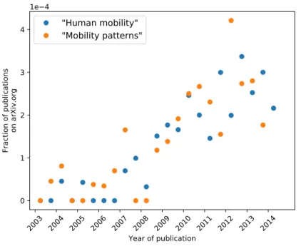
This review predominantly focuses on these later developments. As we will see throughout the text, these new sources of data have rejuvenated the scientific interest for human mobility, opening the door to new questions and measures, as well as en-hancing and validating the insight gained from studying traditional data sources. For reasons which are probably technical, historical, and societal, research teams in physics and computer science have broadly “invested” in these new georeferenced (meta)data resulting from human activity [38]. This is evidenced by a quick search on the online website arXiv1for physics papers that include the terms “Human Mobility” or “Mo-bility Patterns”. As seen in Fig. 2, since about 2004-2005, the number of such papers displays an almost exponential increase. One must keep in mind that this is probably an incomplete sample, and is underestimating the volume of research in this field. It is likely that one would see an even more dramatic trend if a more comprehensive list of
2003 2004 2005 2006 2007 2008 2009 2010 2011 2012 2013 2014
Year of publication
0
1
2
3
4
Fraction of publications
on arXiv.org
1e 4
"Human mobility"
"Mobility patterns"
Fig. 2: Fraction of papers on arXiv.org with mention to the terms ”Human Mobility or ”Mobility Patterns” from 2004 to 2015. The growth in the number of published papers displays a dramatic increase around 2008. Data source: arXiv.org (last date accessed: Feb 16, 2017).
publications were to be included.
While this growing interest of the Physics community in human mobility has mul-tiple reasons, it is somewhat to be expected given the traditional interest of statistical physicists in studying emergent collective properties of systems of many interacting particles and in describing the dynamics of randomly moving particles undergoing (anomalous) diffusion. The availability of data at multiple spatio-temporal scales is helping uncover robust statistical patterns as well as aiding the development of phe-nomenological theories of human mobility, that are well suited to the tools, methods and paradigms of statistical physics.
1.2. Scope and Limitations
The recent pace of developments and the volume of work published are such that a comprehensive review of the findings appeared necessary. Moreover, the study of human mobility is a highly interdisciplinary endeavor and progress has occurred in parallel across different academic communities, sometimes with one unaware of the others’ works. This is reflected in different terminology of common metrics and similar results being cast in different and seemingly unrelated contexts. Consequently with this review, we also aim at (i) bringing disparate communities together by unifying the findings in a common context, and (ii) providing new researchers in the field with an accessible starting point and a minimal set of tools, metrics, concepts and models.
One must note that humans, of course, do not move in a vacuum. Just as the di ffu-sion of molecules in materials is mediated by the structural and thermodynamic prop-erties of the material, similarly, spatio-temporal patterns of human movement are nec-essarily shaped by spatial constraints and limitations of geography. Examples of this are the topography of urban centers or the pattern of roads and transportation infras-tructure, the properties of which are studied under the aegis of spatial networks [39]. Yet, this survey is not about Spatial Networks, nor do we give details on the so-called “science of cities” (e.g., city forms, properties of urban transport networks, urban scal-ing laws, etc. [40]); these two aspects will be considered only when made necessary for the reader to understand the concepts related to human mobility.
1.3. Organization
We begin in Sec. 2 with a comprehensive (but by no means exhaustive) list of data sources used for empirical studies. In Sec. 3 we introduce key metrics, measures, spatio-temporal scales, as well as an overview of the fundamental physics behind the study of human mobility. In Sec. 4 we describe the state-of-the-art families of models (both generative and phenomenological) that best describe the empirical observations of human mobility. The models are categorized according to scale, starting from the level of individuals, through to the collective level of populations, and finally a mixture of the two incorporating the concept of (inter) modality. Continuing with the theme of scales, in Sec. 5 we describe some selected applications of the framework and models ranging from intra-urban movement to flows between countries and continents includ-ing the case of epidemic spreadinclud-ing, transportation systems, and a brief digression on new results on virtual mobility (web browsing). Finally, we conclude in Sec. 6 with challenges and future directions for the field. We also added Appendix A where we provide descriptions of some basic tools and algorithms (agent-based modeling, ran-dom walkers, etc.) that may be of use to researchers making initial forays into the field.
2. Data Sources
A natural starting point is to describe the nature of empirical data which has been used in mobility research. Indeed, empirical data has been vital to both aggregate and individual mobility investigation, by providing means of parameter calibration as well as model validation. In this section, we outline the main sources available for mobility research and the relevant information that can be extracted from them. The data sources are presented in (rough) chronological order of their historical availability and consequent use in research.
2.1. Census Data& Surveys
Census data is collected in periodical national surveys in which householders are asked questions about the socio-demographic and economic status of the household members. Of particular interest in terms of mobility are questions related to the location of the workplace, or the place of current and previous residence. Collectively, this
information can then be used to estimate commuting flows or internal migration flows within a country.
Different countries introduced national censuses at different times, and the type of information collected also varies across countries and time periods. In the United King-dom, for example, the first national census was done in 1841 and contained the names, ages, sexes, occupations, and places of birth of each individual living in a household. In 1921, the location of workplaces was added to the questions asked, and since 1961 the location of previous residence was also included. In the United States, the first pop-ulation census was taken in 1790, while information on workplace and transportation activities was incorporated in 1940 [41]. Nowadays, national censuses are held in most countries typically every ten years. Below we outline some main sources of census and survey data along with the methodology used to extract commuting and migration flows.
2.1.1. Census Data
The data on commuting trips between United States’ counties is available from the United States Census Bureau2. These county-to-county work flow files are available for each state as well as at the aggregated level across the country. Furthermore, files are available in either county of residence format—containing work destinations of people who reside in each county—or county of work format—which contain the county of residence of people working in each county. The inclusion of a commuter in the data is preconditioned upon them working during the week leading up to the census. Due to the questionnaire design, any individual not satisfying this condition is precluded from entering a workplace location. A worker is defined as someone who has spent at least 1 hour in paid employment or 15 hours in a voluntary role. Any individual required to provide their workplace location was asked further questions about their mode of transport and travel time.
From this information, the census Bureau compiles and publishes aggregated flows corresponding to the residence and workplace location of everyone classed as a worker. In order to validate models and determine statistics such as trip distance and relation-ship to the origin, destination and intervening population density, further information on the spatial distribution of counties and socio-demographic data is required. This supporting data is available online3. Among other things, such census data is
invalu-able for validating generative models of commuter flow and migration. For instance, Census data from the 2000s (consisting of county level work flow data, corresponding to 3,141 counties and 34,116,820 commuters within the United States) was used to evaluate the so-called radiation model (described in sec. 4.2.2) by Simini et al. [42]
Commuting and migration flows data for the United Kingdom is also available on-line4. The information is available at different spatial resolutions: ranging from the
geographical area covered by a single postcode, to areas covered by the 7,201 electoral
2http://www.census.gov/hhes/commuting/data/commutingflows.html 3ftp://ftp2.census.gov/geo/tiger/tiger2k/
4http://webarchive.nationalarchives.gov.uk/20160105160709/
http://www.ons.gov.uk/ons/guide-method/census/2011/census-data/ 2011-census-data-catalogue/origin-destination/index.html
Fig. 3: Commuting flows compiled from census data. Left panel: The state of Florida partitioned according to its counties. Right panel: Commuting flows between counties, where thickness of lines correspond to volume of flow. Data compiled from the United States Census Bureau.
wards. Files contain origin and destination flows divided into subsets of age and gender allowing for a deeper socio-demographic analysis if required. There have been many different countries whose commuting data has been analyzed at the level of munici-palities (or smaller administrative units such as zipcodes or electoral tracks) including France5and most European countries. In most cases, when not directly available on an
open data portal, commuting data is available to researchers on request from national statistics institutes.
2.1.2. Tax Revenue Data
An alternative source for estimating aggregated migration flows is the Statistics of Income Division (SOI) of the Internal Revenue Service (IRS) in the United States. The IRS maintains records of all individual income tax forms filed in each year. Using indi-vidual tax return files, it is possible to determine who has, or has not, moved residence or workplace locations in the intervening fiscal year. To do this, first, coded returns for the current filing year are matched to coded returns filed during the prior year. The mailing addresses on the two returns are then compared to one another. If the two are identical, the return is labeled a non-migrant. Any relevant information change during the fiscal year results in the return labeled as that of a migrant. US migration data from 1992-1993 to 2006-2007 is available online6. Alongside tax returns, estimated migra-tions flows are also included in each Census7, based on yearly surveys carried out by the American Community Survey (ACS).
5https://www.insee.fr/fr/statistiques/2022117
6http://www.irs.gov/uac/SOI-Tax-Stats-Migration-Data
2.1.3. Local Travel Surveys
An important source of data used to construct trips, and therefore flows between two locations, is local surveys. It provides an advantage over censuses as it is possi-ble to collect a more detailed data set that includes information such as the purpose of the trip and mode of transport used. However, the increase in accuracy, resolution, and variety of meta-data leads to a corresponding sacrifice in scale. As such, surveys typically have a much lower number of respondents compared to a census. Addition-ally, these typically cover smaller areas such as a single city (or indeed neighborhoods within cities), as opposed to the level of a state, or an entire country.
A representative example is provided by the household Travel Tracker Survey for the Chicago metropolitan area, conducted between 2007 and 2008, and carried out by the Chicago Metropolitan Agency for Planning8. This survey contains information on travel activities of household members, among other details. Information was collected from a total of 10,552 households over a one or two-day period, and households were required to provide a detailed travel inventory for each member, including details such as trip purpose, transport mode, departure and arrival times, and public transport infor-mation such as boarding location, distance to final destination, and fare paid. A similar survey is available for the Los Angeles region9and was analyzed by Liang et al. [43],
where 46,000 trips between 2,017 zones within the Los Angeles county were extracted. The use of small scale surveys is often augmented by other forms of data (for example GPS tracks, see Sec. 2.4) in order to have accurate records of an individual’s position combined with an annotated description of the purposes of each trip [43, 44].
While historically most prevalent, census data provides us only with coarse-grained patterns of human migration and movement. Surveys, on the other hand, provide far more detail but on a much smaller scale, thus limiting their use in terms of statistical validation of models. While the census reveals little information about where people spend their time, or where and how they travel, at the survey level, data reliability is restricted by scale and self-reporting errors. Thus both sources lack the ability to provide a dynamic picture of human mobility [45].
2.2. Dollar Bills
An unusual (and perhaps not immediately apparent) source of mobility data is re-lated to the tracking of currency. An archetypal example of this are online bill-tracking websites, which are designed to monitor the dispersal of individual bank notes world-wide. The movement of a bank note between geographical locations occurs when it is carried by an individual, therefore data collected from such websites may be used to infer trajectories and patterns of human mobility. Brockmann et al. [46] obtained trajectories of 464,670 dollar bills from the website www.wheresgeorge.com, allow-ing for an analysis of bank note dispersal in the United States (excludallow-ing Hawaii and Alaska). The data set contains entries corresponding to time-stamped reports of the geographic location of individual bills, numbering around 250 million as of 2017. All bills registered on the site are initially entered by a user which involves the input of their
8
http://www.cmap.illinois.gov/data/transportation/travel-tracker-survey
©2006Nature Publishing Group
time. Figure 1b shows secondary reports of bank notes with initial entry at Omaha that have dispersed for times T . 100 days (with an average timekTl ¼ 289 days). Only 23.6% of the bank notes travelled farther than 800 km, whereas 57.3% travelled an intermediate dis-tance 50 , r , 800 km, and a relatively large fraction of 19.1% remained within a radius of 50 km, even after an average time of nearly one year. From the computed value Teq< 68 days, a much higher fraction of bills is expected to reach the metropolitan areas of the West coast and the New England states after this time. This is sufficient evidence that the simple Le´vy flight picture for dispersal is incomplete. What causes this attenuation of dispersal?
Two alternative explanations might account for this effect. The slowing down might be caused by strong spatial inhomogeneities of the system. People might be less likely to leave large cities than for example, suburban areas. Alternatively, long periods of rest might be an intrinsic temporal property of dispersal. In as much as an algebraic tail in spatial displacements yields superdiffusive behaviour, a tail in the probability density f(t) for times t between successive spatial displacements of an ordinary random walk can lead to subdiffusion15
(see Supplementary Information). Here, the ambivalence between scale-free spatial displacements and scale-free periods of rest can be responsible for the observed attenuation of superdiffusion.
In order to address this issue we investigated the relative pro-portion Pi
0ðtÞ of bank notes which are reported in a small (20 km)
radius of the initial entry location i as a function of time (Fig. 1d). The quantity Pi
0ðtÞ estimates the probability of a bank note being
reported at the initial location at time t. We computed Pi 0ðtÞ for
metropolitan areas, cities of intermediate size and small towns: for all classes we found the asymptotic behaviour P0(t), At2h, with the same exponent h¼ 0.6 ^ 0.03, which indicates that waiting time and dispersal characteristics are universal. Notice that for a pure Le´vy flight with index b in two dimensions, P0(t) scales with time as t22/b(dashed red line)15. For b< 0.6 (as suggested by Fig. 1c) this
implies h< 3.33. This is a fivefold steeper decrease than observed, which clearly shows that dispersal cannot be described by a pure Le´vy flight. The measured decay is even slower than the decay expected from ordinary two-dimensional diffusion (h¼ 1, dashed black line). Therefore, we conclude that the slow decay in P0(t) reflects the effect
Figure 1 | Dispersal of bank notes and humans on geographical scales. a, Relative logarithmic densities of population (cP¼ logrP/krPl), report
(cR¼ logrR/krRl) and initial entry (cIE¼ logrIE/krIEl) as functions of
geographical coordinates. Colour-code shows densities relative to the nationwide averages (3,109 counties) ofkrPl ¼ 95.15, krRl ¼ 0.34 and
krIEl ¼ 0.15 individuals, reports and initial entries per km2, respectively.
b, Trajectories of bank notes originating from four different places. City names indicate initial location, symbols secondary report locations. Lines represent short-time trajectories with travelling time T , 14 days. Lines are omitted for the long-time trajectories (initial entry in Omaha) with T . 100 days. The inset depicts a close-up view of the New York area. Pie charts indicate the relative number of secondary reports coarsely sorted by distance. The fractions of secondary reports that occurred at the initial entry location (dark), at short (0 , r , 50 km), intermediate (50 , r , 800 km) and long (r . 800 km) distances are ordered by increasing brightness of hue.
The total number of initial entries are N¼ 2,055 (Omaha), N ¼ 524
(Seattle), N¼ 231 (New York), N ¼ 381 (Jacksonville). c, The short-time
dispersal kernel. The measured probability density function P(r) of traversing a distance r in less than T¼ 4 days is depicted in blue symbols. It is computed from an ensemble of 20,540 short-time displacements. The dashed black line indicates a power law P(r),r2(1þ b)with an exponent of
b¼ 0.59. The inset shows P(r) for three classes of initial entry locations (black triangles for metropolitan areas, diamonds for cities of intermediate size, circles for small towns). Their decay is consistent with the measured exponent b¼ 0.59 (dashed line). d, The relative proportion P0(t) of
secondary reports within a short radius (r0¼ 20 km) of the initial entry
location as a function of time. Blue squares show P0(t) averaged over 25,375
initial entry locations. Black triangles, diamonds, and circles show P0(t) for
the same classes as c. All curves decrease asymptotically as t2hwith an
exponent h¼ 0.60 ^ 0.03 indicated by the blue dashed line. Ordinary
diffusion in two dimensions predicts an exponent h¼ 1.0 (black dashed
line). Le´vy flight dispersal with an exponent b¼ 0.6 as suggested by b predicts an even steeper decrease, h¼ 3.33 (red dashed line).
NATURE|Vol 439|26 January 2006 LETTERS
463
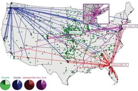
Fig. 4: Trajectories of bank notes originating from four different locations. Tags indicate initial, symbols secondary report locations. Lines represent short time trajectories with traveling time T < 14 days. Lines are omitted for the long time trajectories (initial entry: Omaha) with T > 100 days. The inset depicts a close-up of the New York area. Pie charts indicate the relative number of secondary reports coarsely sorted by distance. The fractions of secondary reports that occurred at the initial entry location (dark), at short (0 < r < 50km), intermediate (50 < r < 800km) and long (r > 800km) distances are ordered by increasing brightness of hue. The total number of initial entries are N= 2, 055 (Omaha), N = 524 (Seattle), N = 231 (New York), N= 381 (Jacksonville). Figure from [46].
ZIP code and a serial number printed on the bill. While the majority of the bills are not entered more than once, around 11% of the bills are reported multiple times, with 3-5 entries per bill being fairly common (Any more than 5 entries is considered rare). Once a bill has been registered, any future hits allow for time and distance between reports to be determined and recorded in the database (see Fig. 4).
While a convenient and large-scale source of mobility data, the use of currency to infer patterns in human mobility is problematic. For instance, bank note dispersals do not contain information on the number of individuals that have carried a given note dur-ing two instances of measurement (i.e., when it appears in the database). Consequently, the trajectories of bank notes are likely a convolution of the mobility of several indi-viduals; coupled with the relatively few samples per dollar bill, this makes it a rather inaccurate and problematic source for inferring individual mobility patterns. Never-theless, similar to census data, currency tracking provides a convenient, and relatively easily accessible picture of the coarse-grained patterns of human mobility.
2.3. Mobile Phone Records
Perhaps the most important, game-changing data of the last decade for inferring human mobility are the mobile phone Call Detail Records (CDRs). Most cell phone companies maintain detailed records of customer information related to their calls and text messages. The information contained in these CDRs include the time of the
Fig. 5: Trajectories of two anonymized mobile phone users traveling in the vicinity of N = 22 and 76 different cell phone towers during a 3-month-long observational period. Each dot corresponds to a mobile phone tower, and each time a user makes a call, the closest tower that routes the call is recorded, pinpointing the users approximate location. The gray lines represent the Voronoi lattice, approximating each towers area of reception. The colored lines represent the recorded movement of the user between the towers. Figure from [47].
call/message as well as the company’s cell tower routing the communication. Know-ing the exact geographic coordinates of the cell tower makes it possible to estimate the approximate location of the user. As mobile phones are (typically) personal de-vices and are mostly carried by a single person, the corresponding location data can be used to infer a single individual’s movements over the recorded period (an example is shown in Fig. 5). Unlike the census, surveys, or currency tracking, CDRs allow for the characterization of individual mobility patterns, and – depending on the dataset – at an unprecedented spatio-temporal resolution. Furthermore, due to the tremendous trend of global cell-phone adoption, one can conduct multi-scale studies ranging from the level of neighborhoods to the country-wide level (including international travel and movement across borders).
CDR data concern both phone calls and SMS exchange and always include the following information: time stamp, caller ID, recipient ID, call duration and antenna (cellular tower) code. Due to privacy concerns, customer identifiers are anonymized before the data is made available to scientists for analysis. Quite often, additional clean up of the data is required to make the data more analyzable; for instance, one typically needs to restrict the dataset to users who visit a minimum threshold number of towers, as well as make calls at a high enough frequency to maintain statistical reliability for each user.
One of the first work using CDR’s was performed by Gonzal´ez et al. [48] on two anonymized datasets provided by a major mobile operator in a large European country. The first set contained the locations of 100,000 randomly selected mobile users whose positions were recorded over a period of 6 months, each time a call or text was received or sent. The second set (collected for validation purposes) corresponded to the locations of 206 mobile users, recorded every two hours over a period of a week. From this
data, traces of mobility patterns such as the distribution of displacements between the locations of consecutive calls (jump-lengths) were measured. The temporal period between consecutive calls was also measured to determine a distribution of wait times (i.e., characteristic time spent by users in a given location). The knowledge of users’ consecutive locations also enabled the calculation of so-called return time distributions, measuring the probability of a user to return to a given location within a given time. Other more complex metrics, including the radius of gyration were also extracted. (For details on metrics see Sec. 3.1).
The quality of mobility information extracted from mobile phone data depends on the frequency at which the location of the user is recorded. For example, the larger data set used in [48] displayed an irregular call pattern; many calls were placed over a short time period, followed by long periods of inactivity. Consequently, the data dis-played a highly inconsistent temporal frequency, which may confound the analysis of mobility patterns. The smaller-scale validation dataset was therefore collected to ac-count for these irregularities. Other problematic issues also arise, such as the accuracy of recorded locations. In general, it is the position of the cell tower routing the call that is recorded and not the exact location of the individual carrying the phone. Since there is significant variability in the areas covered by cell towers—with coverage ranging from tens of meters in the densest neighborhoods of urban areas, to a few kilometers in rural areas—a recorded user in a rural area may transmit all communication via a single tower during their daily routine, while moving the exact same area as that of an urban user who may ping several towers. Thus, in the former case, despite possibly significant movement on part of the user, for purposes of analysis they are considered stationary, which is obviously misleading.
We must note that obtaining CDRs for research purposes poses significant chal-lenges. Since they are not typically publicly available, one has to directly approach a mobile phone operator. As the data contains sensitive information [49], any data col-lected by a specific group of researchers may not be shared with other groups, making reproducibility problematic. Yet, recent initiatives have seen some phone companies release large scale CDR data within the context of ”challenges” among researchers. The purpose of making this data available is to provide researchers some material al-lowing them to extract useful information to address major societal challenges. Such recent datasets are those that have been provided by Orange in the framework of their Data 4 Development (D4D) challenge. These contain four anonymized tables for mo-bile phone users in the Ivory Coast (Cˆote d’Ivoire) and Senegal. For example, in the case of Ivory Coast, data contained (i) hourly antenna-to-antenna traffic; (ii) individual trajectories of 50,000 users over two weeks with antenna location information; (iii) in-dividual trajectories of 500,000 users over an entire year with sub-prefecture location information; (iv) communication graphs for 5,000 users [50]. In particular (iii) con-tains information regarding individual trajectories for the entire observation period at the cost of reduced spatial resolution; position is recorded as a sub-prefecture rather than antenna location. The raw data consists of a user ID, date and time stamp of the communication and the sub-prefecture number (1-255) which can be linked to a file containing the latitude and longitude of the center of each sub-prefecture [51].
Telecom Italia’s “Big Data Challenge” is another example of a large scale CDR data set readily available to researchers. Alongside anonymized call records,
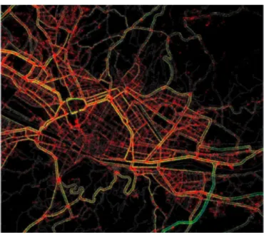
addi-Fig. 6: Aggregated GPS position data (collected from vehicles) in a part of Florence, Italy, measured during March 2008; the red dots correspond to a recorded instantaneous velocity ≤ 30 km h−1, whereas the yellow
dots correspond to velocities in the interval 30 − −60 km h−1and the green dots to a velocity ≥ 60 km h−1.
Figure from [57].
tional metadata related to weather, news, Twitter activity, and electricity data from two areas in Italy (Milan and Trentino) was provided [52]. Data from this challenge has been used to investigate the relationship between individual daily trips and personal constraints [53], estimate urban population from call volume [54] or determine the rela-tionship between urban communication and happiness [55]. The increasing availability of such large-scale, anonymized datasets for research purposes is an encouraging trend for future research on human mobility. For more detailed information on CDR sources and some associated results (including other research topics than human mobility), see the review by Blondel et al. [56].
2.4. GPS Data
The greatest level of accuracy on movement trajectories is provided by Global Po-sitioning System (GPS) data, which is capable of providing precise information on any location covered by at least four GPS Satellites. GPS trackers are units which receive signals from GPS satellites and compute the device’s position at regular intervals. This technology allows researchers to trace the movement of individuals with a high degree of accuracy and temporal frequency, thus providing a rich source of data that can be analyzed and directly mapped to human mobility patterns.
Rhee et al. [58] used GPS trackers with a position accuracy of less than three me-ters to record the movements of over 150 individuals across two University campuses, a state fair (US), Disney World, and New York City. The position of the individuals
carrying the trackers was recorded every 10 seconds while they were in these locations resulting in daily traces that had on average a temporal scale of 9-10 hours. Addition-ally, Microsoft has made GPS trajectories from 182 individuals freely available online via their GeoLife project10. The dataset consists of 17,621 trajectories recorded by GPS trackers and GPS enabled mobile devices, and has a high spatial and temporal scale for over 90% of individuals with positions recorded every 1-5 seconds or 5-10 meters for time periods that span several years. Since its release, GeoLife has been used in studies of both human mobility [59, 60] and social interactions [61]. For a review of potential applications see [62].
Transmitters attached to vehicles [63, 64] are another source of GPS data. These are useful for studying questions related to urban traffic: monitoring, prediction, and pre-vention of congestion [64]. In Italy, ' 2% of privately owned cars have a GPS system; each vehicle has assigned a unique identifying number, thus enabling the tracing of anonymous individual cars’ trajectories with high precision. A GPS signal is transmit-ted approximately every 2km, as well as when the engine is switched on and off [63]. Each signal is converted to a data point containing information on position, velocity and distance covered. While the data suffers from inaccuracy due to variables such as satellite coverage and position precision, the temporal precision is of high quality, as is both instantaneous velocity and distance covered. From such GPS vehicle traces, path length distributions can be measured, which corresponds to the distribution of distances traveled in single trips, where a trip is defined as travel that occurs between instances of the engine being started and stopped. Activity distributions, which are equivalent to waiting time distributions in other studies, can also be determined from the elapsed time between consecutive trips. A further advantage of GPS traces over CDRs is that the locations are recorded to a much higher degree of accuracy and at a constant fre-quency. Yet, there are drawbacks: GPS transmitters do not work indoors and generally rely on batteries as their source of power. As a result, traces can contain periods dur-ing which no signal is received or may be terminated prematurely. Furthermore, GPS datasets typically feature a smaller number of individual users, up to several thousand, in comparison to mobile phone data which can provide information on the mobility of millions of users.
2.5. Online Data
Another valuable source of location information are Online Social Network (OSN) or Location-Based Social Network (LBSN) services, that attract hundreds of millions of users worldwide. Since the introduction of GPS and wifi chips in smartphones, social network providers have been able to collect valuable data on both the social con-nections as well as precise geographical locations of their users. Indeed, services such as Twitter, Facebook, Foursquare and Flickr collect geotagged data every time a user enables localization for the content being posted (e.g., checking-in at a restaurant with friends); this is associated with geographic coordinates, a time stamp, and additional information relative to the location itself or the content published by the user. The mobility profiles of the users can be obtained from the list and number of locations
Fig. 7: Country-specific analyses of travel based on Twitter users and on the estimated total number of travelers. Panel A shows the number of Twitter users residing in a country and traveling to another while panel B shows the number of users visiting this particular country. Panels C and D represent the number of Twitter travelers normalized by the extent of Twitter usage in their home country. Finally panel E represents the yearly ratio between the estimated inflow and outflow of travelers, revealing which countries were the origin or destination of international travel. Figure from [66].
other than their home which they have visited over the period of the study (see Fig. 7 for an example). These profiles can range from intra-urban routine trips to worldwide travel [65, 66]. From the geographical locations, by inferring a user’s home location, their radius of gyration can be determined using the geographical distance between the home location and reported locations. The jump length distribution can be determined by defining a jump as the geographical distance between consecutive reports for a sin-gle user and frequency of reports can be used to assess temporal patterns in human mobility [66]. Other measures such as visitation frequency and predictability are also obtainable [67].
Geotagged data can also be used to assess social interactions between individuals. Scellato et al. [68] analyzed three online location-based social networks: Foursquare, Brightkite, and Gowalla, finding their exhibition of common properties found in most other real world complex networks, such as fat tailed degree distributions, high clus-tering coefficient, and short average path length between nodes, confirming the small-world nature of LBSN’s [69]. Furthermore, the probability of a social link between two users was found to exhibit a distance dependence, decreasing with geographical separation between the users. Compared to CDR’s, data collected from OSN’s and LBSN’s, have the advantage of having more contextual information associated with the geographical positions and the users, enabling the study of mobility in a broader context. For example, data collected from Twitter users has been applied to topics such as social networks [70, 71, 72], evolution of moods [73, 74, 75], and crisis manage-ment [76, 77, 78] among other features.
Yet, as in all other data sources, limitations persist. Besides requiring extensive clean up (such as removing users with suspiciously high activity, unreasonably fast movement between two consecutive check-ins or incomplete data [66]), mobility and interaction data originating from online social networks needs further validation in or-der to be consior-dered truly representative of the general population. Sloan et al. [79] found that Twitter data originating from the UK has significant demographic di ffer-ences compared to the wider population data from UK census. Furthermore, there appear to be demographic differences between the users who enable geotagging and those who do not (only ≈ 3% of the users were found to have geotagging enabled). 3. Metrics, Physics and Scales
In this section, we will discuss some of the fundamental metrics used to character-ize mobility as well as the associated spatio-temporal scales at which they are relevant. We will then move onto a discussion of some of the physics associated with mobility, including the relations between distance, time and velocity. We end the section with a discussion of energy arguments and interpolation of spatio-temporal scales through the lens of multimodality.
3.1. General Metrics 3.1.1. Jump Lengths
A key factor in modeling human mobility is the distance an individual travels in a given time period. Measures of distance are often dependent on the source of data being used, and the terms flight length, jump length, displacement, and trip refer to dif-ferent distance measures that may be extracted from data. For example, early measures of mobility leveraged information about the spatial trajectories of bank-notes (one can think of this as an aggregation of many individual trips as a given banknote necessar-ily changes many hands). Conventionally, the distance between two instances of the appearance of a banknote in the measured data is termed a jump length [46]. Later, higher resolution measurements of movement were provided by Call Detail Records (CDRs). Here one could reliably measure the location (and corresponding displace-ment) of individuals based on placement of mobile phone towers that are pinged when one makes a call. Associated with the displacement between two successive calls is a time interval [48], that provides an estimate of the stay of an individual in a lo-cation (waiting-times), although it is not possible to detect the position of the user between two consecutive calls. Even higher resolution spatio-temporal data available from Global Positioning System (GPS) allows one to make more stringent definitions of displacement. In addition to the standard definition of jump-lengths [58], one can now define a displacement between stops, i.e. the displacement of individuals between two locations, given that they spent a minimum amount of time per location [63]. In-deed, the use of the terms “stop”, “trip” or “displacement” reflects human behavioral tendencies that motivate people to go from point A to point B. It is therefore important to verify that a “stop” corresponds to an actual behavior and that it is not artificially generated by oversampled or undersampled signals [80].
Regardless of how one chooses to constrain it, the jump length, typically denoted as∆r, is defined as the euclidean distance between r(t) and r(t + dt) corresponding to
locations recorded at intervals t and t+ dt. Of particular interest is the distribution of ∆r within a population; how likely is it that a random member of the population will travel a distance r from their origin location in a time dt? In order to measure this, when modeling human mobility it is common to consider the probability distribution function (PDF) of jump lengths, P(∆r). This may be defined as the probability of finding a displacement∆r in a short time step dt.
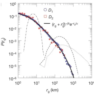
Brockmann et al. [46] determined P(∆r) for the trajectories of dollar bills and the distribution of jump lengths was observed to follow a power law, P(∆r) ∼ ∆r−(1+β),
with exponent β = 0.59 ± 0.02, independent of the size (in population) of the entry point of a bank note (see Fig. 8). The power-law behavior of P(∆r) has also been ob-served in the trajectories of mobile phone users [48, 81]. The empirical distribution of displacements obtained from mobile phone data analyzed in [48] is well approximated by a truncated power-law distribution:
P(∆r) = (∆r − ∆r0)−(1+β)exp (−∆r/κ) (5)
where r0 and κ represent cutoffs at small and large values of ∆r. The value of the
observed scaling exponent in Eq. (5) is β= 0.75 ± 0.15, not far from β = 0.59 ± 0.02 obtained from bank note dispersal, suggesting that the two distributions may capture the same fundamental mechanism driving human mobility patterns. Zhao et al. [82] measured the distribution of jump lengths using two GPS data sets that, along with location and time stamps, also included transportation mode. From this, the jump length∆r was determined as the longest straight line distance between two locations without a change of direction. Wait times,∆t, were taken to be the time spent in a particular transportation mode. A single trip may be made up of several flights, each of which have a corresponding transportation mode taken directly from the dataset. The transportation modes were grouped into four categories; Walk/Run, Car/Bus/Taxi, Subway/Train and Bike. The distribution of jump lengths is found to be log-normal if each transportation mode is considered individually, whereas P(∆r) for all modes combined follows a truncated power-law with β= 0.55 and 0.39 for the two datasets. The distribution of wait times, P(∆t), was found to be exponential, corresponding to a large number of Walk/Run flights that connect the use of other transportation modes within a single trip and therefore have only a short duration. This result provides further insight into studies using on bank note and mobile phone data [46, 48, 81] in that the power-law behavior of the distribution of jump lengths is the result of combining several distinct log-normal distributions, corresponding to the different transportation modes available, with exponentially distributed wait times. GPS devices installed in cars transmit the location of the car to a high degree of accuracy every few seconds when the car is in motion. The analysis of such data from over 150,000 cars in Italy over a period of one month [64] found that the probability density function, P(∆r) had two different regimes; an exponential distribution up to a characteristic distance of ∼20 km corresponding to inter-city travels, and a power-law with β= 1.53 corresponding to intra-city movement. Here,∆r corresponds to the true length of a single trip. Trips are distinguished by records that are greater than 20 mins apart; as the GPS device only transmits when the car is moving, using a threshold of 20 mins allows for small stops, such as waiting at traffic lights or re-fueling, to be accounted for and included within a single trip. The exponent, β, is significantly higher than those obtained for bank note
time. Figure 1b shows secondary reports of bank notes with initial
entry at Omaha that have dispersed for times T . 100 days (with an
average time
kTl ¼ 289 days). Only 23.6% of the bank notes travelled
farther than 800 km, whereas 57.3% travelled an intermediate
dis-tance 50 , r , 800 km, and a relatively large fraction of 19.1%
remained within a radius of 50 km, even after an average time of
nearly one year. From the computed value Teq
< 68 days, a much
higher fraction of bills is expected to reach the metropolitan areas of
the West coast and the New England states after this time. This is
sufficient evidence that the simple Le´vy flight picture for dispersal is
incomplete. What causes this attenuation of dispersal?
Two alternative explanations might account for this effect. The
slowing down might be caused by strong spatial inhomogeneities of
the system. People might be less likely to leave large cities than for
example, suburban areas. Alternatively, long periods of rest might be
an intrinsic temporal property of dispersal. In as much as an algebraic
tail in spatial displacements yields superdiffusive behaviour, a tail in
the probability density f(t) for times t between successive spatial
displacements of an ordinary random walk can lead to subdiffusion
15(see Supplementary Information). Here, the ambivalence between
scale-free spatial displacements and scale-free periods of rest can be
responsible for the observed attenuation of superdiffusion.
In order to address this issue we investigated the relative
pro-portion P
i0ðtÞ of bank notes which are reported in a small (20 km)radius of the initial entry location i as a function of time (Fig. 1d).
The quantity P
i0ðtÞ estimates the probability of a bank note beingreported at the initial location at time t. We computed P
i0ðtÞ formetropolitan areas, cities of intermediate size and small towns: for all
classes we found the asymptotic behaviour P
0(t)
, At
2h, with the
same exponent h
¼ 0.6 ^ 0.03, which indicates that waiting time
and dispersal characteristics are universal. Notice that for a pure
Le´vy flight with index b in two dimensions, P
0(t) scales with time
as t
22/b(dashed red line)
15. For b
< 0.6 (as suggested by Fig. 1c) this
implies h
< 3.33. This is a fivefold steeper decrease than observed,
which clearly shows that dispersal cannot be described by a pure Le´vy
flight. The measured decay is even slower than the decay expected
from ordinary two-dimensional diffusion (h
¼ 1, dashed black line).
Therefore, we conclude that the slow decay in P
0(t) reflects the effect
Figure 1 | Dispersal of bank notes and humans on geographical scales.
a, Relative logarithmic densities of population (c
P¼ logrP
/kr
Pl), report(c
R¼ logrR
/kr
Rl) and initial entry (cIE¼ logr
IE/kr
IEl) as functions ofgeographical coordinates. Colour-code shows densities relative to the
nationwide averages (3,109 counties) of
kr
Pl ¼ 95.15, kr
Rl ¼ 0.34 and
kr
IEl ¼ 0.15 individuals, reports and initial entries per km
2, respectively.
b, Trajectories of bank notes originating from four different places. City
names indicate initial location, symbols secondary report locations. Lines
represent short-time trajectories with travelling time T , 14 days. Lines are
omitted for the long-time trajectories (initial entry in Omaha) with
T . 100 days. The inset depicts a close-up view of the New York area. Pie
charts indicate the relative number of secondary reports coarsely sorted by
distance. The fractions of secondary reports that occurred at the initial entry
location (dark), at short (0 , r , 50 km), intermediate (50 , r , 800 km)
and long (r . 800 km) distances are ordered by increasing brightness of hue.
The total number of initial entries are N
¼ 2,055 (Omaha), N ¼ 524
(Seattle), N
¼ 231 (New York), N ¼ 381 (Jacksonville). c, The short-time
dispersal kernel. The measured probability density function P(r) of
traversing a distance r in less than T
¼ 4 days is depicted in blue symbols.
It is computed from an ensemble of 20,540 short-time displacements. The
dashed black line indicates a power law P(r),r
2(1þ b)with an exponent of
b
¼ 0.59. The inset shows P(r) for three classes of initial entry locations
(black triangles for metropolitan areas, diamonds for cities of intermediate
size, circles for small towns). Their decay is consistent with the measured
exponent b
¼ 0.59 (dashed line). d, The relative proportion P
0(t) of
secondary reports within a short radius (r
0¼ 20 km) of the initial entry
location as a function of time. Blue squares show P
0(t) averaged over 25,375initial entry locations. Black triangles, diamonds, and circles show P
0(t) for
the same classes as c. All curves decrease asymptotically as t
2hwith an
exponent h
¼ 0.60 ^ 0.03 indicated by the blue dashed line. Ordinary
diffusion in two dimensions predicts an exponent h
¼ 1.0 (black dashed
line). Le´vy flight dispersal with an exponent b
¼ 0.6 as suggested by b
predicts an even steeper decrease, h
¼ 3.33 (red dashed line).
NATURE|Vol 439|26 January 2006
LETTERS
Fig. 8: The short-time dispersal kernel of bank notes. The measured probability density function P(r) of traversing a distance r in less than T = 4 days is depicted in blue symbols. It is computed from an ensemble of 20,540 short-time displacements. The dashed black line indicates a power law P(r) ∼ r−(1+β) with an exponent of β ∼ 0.59. The inset shows P(r) for three classes of initial entry locations (black triangles for metropolitan areas, diamonds for cities of intermediate size, circles for small towns). Their decay is consistent with the measured exponent β= 0.59 (dashed line). Figure from [46].
dispersal [46] and mobile phone data [48, 81]. The authors suggest this is due to the limitation in the GPS data caused by restrictions on the size of the area covered (500km in length), and the physical limitation on the distance an individual will drive in a single trip.
3.1.2. Mean Square Displacement (MSD)
Research into the distribution of jump lengths suggests that individual trajectories can be described by L´evy flights, a family of models associated with random walks (described in detail in Sec. 4.1). In this context, a common measure of the potential exploration of area by an individual is the Mean Square Displacement (MSD):
MSD(t)= h(r(t) − r0)2i ≡ h∆r(t)2i. (6)
Here r0is a vector marking the origin of the individual relative to some reference point,
or in other words, the location at which a particular trajectory starts, while r(t) mea-sures the subsequent position of the individual at time t. The scaling of MSD with time provides a measure of the type of diffusion of individuals relative to their starting point in a trip. The MSD(t) has the unit of an area and it corresponds to the average squared distance from the origin after a time t. In general, if the individual mobility trajectories follow a so-called Continuous Time Random Walk, (Cf. Sec. 4.1.3), the MSD follows the form h∆r(t)2i ∼ tνwith ν= 2α/β where α and β are the exponents of the
waiting-time, i.e. the time interval between two consecutive jumps, and jump length PDFs [46].