HAL Id: hal-01389137
https://hal.archives-ouvertes.fr/hal-01389137
Submitted on 3 Nov 2016
HAL is a multi-disciplinary open access
archive for the deposit and dissemination of
sci-entific research documents, whether they are
pub-lished or not. The documents may come from
teaching and research institutions in France or
abroad, or from public or private research centers.
L’archive ouverte pluridisciplinaire HAL, est
destinée au dépôt et à la diffusion de documents
scientifiques de niveau recherche, publiés ou non,
émanant des établissements d’enseignement et de
recherche français ou étrangers, des laboratoires
publics ou privés.
Distributed under a Creative Commons Attribution - NonCommercial| 4.0 International
License
Pushing the Limits of Online Auto-tuning: Machine
Code Optimization in Short-Running Kernels
Fernando Endo, Damien Couroussé, Henri-Pierre Charles
To cite this version:
Fernando Endo, Damien Couroussé, Henri-Pierre Charles. Pushing the Limits of Online Auto-tuning:
Machine Code Optimization in Short-Running Kernels. Proceedings of MCSOC 2016. IEEE 10th
In-ternational Symposium on Embedded Multicore/Many-core Systems-on-Chip (MCSoC-16), Sep 2016,
Lyon, France. �hal-01389137�
Pushing the Limits of Online Auto-tuning: Machine
Code Optimization in Short-Running Kernels
Fernando Endo, Damien Courouss´e, Henri-Pierre Charles
Univ. Grenoble Alpes, F-38000 Grenoble, France / CEA, LIST, MINATEC Campus, F-38054 Grenoble, France
Abstract—This article proposes an online auto-tuning ap-proach for computing kernels. Differently from existing online auto-tuners, which regenerate code with long compilation chains from the source to the binary code, our approach consists on deploying auto-tuning directly at the level of machine code generation. This allows auto-tuning to pay off in very short-running applications. As a proof of concept, our approach is demonstrated in two benchmarks, which execute during hundreds of milliseconds to a few seconds only. In a CPU-bound kernel, the speedups achieved are 1.10 to 1.58 in average depending on the target micro-architecture, up to 2.53 in the most favourable conditions (all run-time overheads included). In a memory-bound kernel, less favourable to our runtime auto-tuning optimizations, the speedups are 1.04 to 1.10 in average, up to 1.30. Despite the short execution times of our benchmarks, the overhead of our runtime auto-tuning is between 0.2 and 4.2 % only of the total application execution times. By simulating the CPU-bound application in 11 different CPUs, we showed that, despite the clear hardware disadvantage of In-Order (IO) cores vs. Out-of-Order (OOO) equivalent cores, online auto-tuning in IO CPUs obtained an average speedup of 1.03 and an energy efficiency improvement of 39 % over the SIMD reference in OOO CPUs.
I. INTRODUCTION
High-performance general-purpose embedded processors are evolving with unprecedented grow in complexity. ISA back-compatibility and energy reduction techniques are among the main reasons. For sake of software development cost, applications do not necessarily run in only one target, one binary code may run in processors from different manufacturers and even in different cores inside a SoC.
Iterative optimization and auto-tuning have been used to automatically find the best compiler optimizations and algorithm implementations for a given source code and target CPU. These tuning approaches have been used to address the complexity of desktop- and server-class processors (DSCPs). They show moderate to high performance gains compared to non-iterative compilation, because default compiler options are usually based on the performance of generic benchmarks executed in representative hardware. Usually, such tools need long space exploration times to find quasi-optimal machine code. Previous work addressed auto-tuning at run-time [1], [2], [3], [4], however previously proposed auto-tuners are only adapted to applications that run for several minutes or even hours, such as scientific or data center workload, in order to pay off the space exploration overhead and overcome the costs of static compilation.
While previous work proposed run-time auto-tuning in DSCP, no work focused on general-purpose embedded-class processors.
In hand-held devices, applications usually run for a short period of time, imposing a strong constraint to run-time auto-tuning systems. In this scenario, a lightweight tool should be employed to explore pre-identified code optimizations in computing kernels.
We now explain our motivation for developing run-time auto-tuning tools for general-purpose embedded processors:
Embedded core complexity. The complexity of high-performance embedded processors is following the same trend as the complexity of DSCP evolved in the last decades. For example, current 64-bit embedded-class processors are sufficiently complex to be deployed in micro-servers, eventually providing a low-power alternative for data center computing. In order to address this growing complexity and provide better performance portability than static approaches, online auto-tuning is a good option.
Heterogeneous multi/manycores. The power wall is affecting embedded systems as they are affecting DSCP, although in a smaller scale. Soon, dark silicon may also limit the powerable area in embedded SoC. As a consequence, heterogeneous clusters of cores coupled to accelerators are one of the solutions being adopted in embedded SoC. In the long term, this trend will exacerbate software challenges of extracting the achievable computing performance from hardware, and run-time approaches may be the only way to improve energy efficiency [5].
ISA-compatible processor diversity. In the embedded mar-ket, a basic core design can be implemented by different manufacturers with different transistor technologies and also varying configurations. Furthermore, customized pipelines may be designed, yet being entirely ISA-compatible with basic designs. This diversity of ISA-compatible embedded processors facilitates software development, however because of differences in pipeline implementations, static approaches can only provide sub-optimal performance when migrating between platforms. In addition, contrary to DSCP, in-order (IO) cores are still a trend in high-performance embedded devices because of low-power constraints, and they benefit more from target-specific optimizations than out-of-order (OOO) pipelines. Static auto-tuning performance is target-specific. In average, the performance portability of statically auto-tuned code is poor when migrating between different micro-architectures [6]. Hence, static auto-tuning is usually employed when the execution environment is known. On the other hand, the trends of hardware virtualization and software packages in general-purpose processors result in applications underutilizing the
hardware resources, because they are compiled to generic micro-architectures. Online auto-tuning can provide better performance portability, as previous work showed in server-class processors [4].
Ahead-of-time auto-tuning. In recent Android versions (5.0 and later), when an application is installed, native machine code is generated from bytecode (ahead-of-time compilation). The run-time auto-tuning approach proposed in this work could be extended and integrated in such systems to auto-tune code to the target core(s) or pre-profile and select the best candidates to be evaluated in the run-time phase. Such approach would allow auto-tuning to be performed in embedded applications with acceptable ahead-of-time compilation overhead.
Interaction with other dynamic techniques. Some powerful compiler optimizations depend both on input data and the target micro-architecture. Constant propagation and loop unrolling are two examples. The first can be addressed by dynamically specializing the code, while the second is better addressed by an auto-tuning tool. When input data and the target micro-architecture are known only at program execution, which is usually the case in hand-held devices, mixing those two dynamic techniques can provide even higher performance improvements. If static versioning is employed, it could easily lead to code size explosion, which is not convenient to embedded systems. Therefore, run-time code generation and auto-tuning is needed.
This article proposes an online auto-tuning approach for computing kernels in ARM processors. Existing online auto-tuners regenerate code using complex compilation chains, which are composed of several transformation stages to transform source into machine code, leading to important compilation times. Our approach consists on shortening the auto-tuning process, by deploying auto-tuning directly at the code generation level, through a run-time code generation tool, called deGoal [7]. This allows auto-tuning to be successfully employed in very short-running kernels, thanks to the low run-time code generation overhead. Our very fast online auto-tuner that can quickly explore the tuning space, and find code variants that are efficient on the running micro-architecture. The tuning space can have hundreds or even thousands of valid binary code instances, and hand-held devices may execute applications that last for a few seconds. Therefore, in this scenario online auto-tuners have a very strong timing constraint. Our approach address this problem with a two-phase online exploration and by deploying auto-tuning directly at the level of machine code generation.
The proposed approach is evaluated in a highly CPU-bound (favorable) and a highly memory-CPU-bound (unfavorable) application, to be representative of all applications between these two extreme conditions. In ARM platforms, the two benchmarks run during hundreds of milliseconds to only a few seconds. In the favorable application, the average speedup is 1.26 going up to 1.79, all run-time overheads included.
One interesting question that this work tries to answer is if run-time auto-tuning in simpler and energy-efficient cores can
obtain performance similar to statically compiled code run in more complex and hence power-hungry cores. The aim is to compare the energy and performance of IO and OOO designs, with the same pipeline and cache configurations, except for the dynamic scheduling capability. This study would tell us at what extent run-time auto-tuning of code can replace OOO execution. However, given that commercial IO designs have less resources than OOO ones (e.g., smaller caches, branch predictor tables), a simulation framework was employed to perform this experiment. The simulation results show that online micro-architectural adaption of code to IO pipelines can in average outperform the hand vectorized references run in similar OOO cores: despite the clear hardware disadvantage, the proposed approach applied to the CPU-bound application obtained an average speedup of 1.03 and an energy efficiency improvement of 39 %.
II. MOTIVATIONAL EXAMPLE
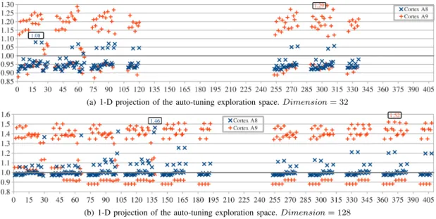
In this section, we present an experiment supporting the idea that performance achievements could be obtained by the combined use of run-time code specialization and auto-tuning. The experiment is carried out with a SIMD version of the euclidean distance kernel implemented in the Streamcluster benchmark, manually vectorized in the PARVEC [8] suite (originally from the PARSEC 3.0 suite [9]). In the reference kernel, the dimension of points is a run-time constant, but given that it is part of the input set, compilers cannot optimize it. In the following comparisons, we purposefully set the dimension as a compile-time constant in the reference code to let the compiler (gcc 4.9.3) generate highly optimized kernels (up to 15 % of speedup over generic versions). This ensures a fair comparison with auto-tuned codes. With deGoal [7], in an offline setting, we generated various kernel versions, by specializing the dimension and auto-tuning the code implementation for an ARM Cortex-A8 and A9. The auto-tuned parameters mainly affect loop unrolling and pre-fetching instructions, and are detailed in Section III-A. Figure 1 shows the speedups of various generated kernels in the two core configurations. By analyzing the results, we draw several motivating ideas:
Code specialization and auto-tuning provide considerable speedups even compared to statically specialized and manually vectorized code: Auto-tuned kernel implementations obtained speedups going up to 1.46 and 1.52 in the Cortex-A8 and A9, respectively.
The best set of auto-tuned parameters and optimizations varies from one core to another: In both cases in Figure 1, there is a poor performance portability of the best configurations between the two cores. For example, in Figure 1(b), when the best kernel for the Cortex-A8 is executed in the A9, the execution time increases by 55 %, compared to the best kernel for the latter. Conversely, the best kernel for the A9 when executed in the A8 increases the execution time by 21 %, compared to the most performing kernel.
There is no performance correlation between the sets of optimizations and input data: The main auto-tuned parameters
(a) 1-D projection of the auto-tuning exploration space. Dimension = 32
(b) 1-D projection of the auto-tuning exploration space. Dimension = 128
Fig. 1: Speedups of euclidean distance kernels statically generated with deGoal. The reference is a hand vectorized kernel (from PARVEC) compiled with gcc 4.9.3 and highly optimized to each target core (-O3 and -mcpu options). Both deGoal and reference kernels have the dimension of points specialized (i.e. set as a compile-time constant). The exploration space goes beyond 600 configurations, but here it was zoomed in on the main region. The peak performance of each core is labeled. Empty results in the exploration space correspond to configurations that could not generate code.
are related to loop unrolling, which depends on the dimension of points (part of the input set). In consequence, the exploration space and the optimal solution depend on an input parameter. For example, the configurations of the top five peak perfor-mances for the A8 in Figure 1(b) (configurations 30, 66, 102, 137 and 138) have poor performances in Figure 1(a) or simply can not generate code with a smaller input set.
The results suggest that, although code specialization and auto-tuning provide high performance improvements, they should ideally be performed only when input data and target core are known. In the released input sets for Streamcluster, the dimensions are 32, 64 and 128, but the benchmark accepts any integer value. Therefore, even if the target core(s) was (were) known at compile time and the code was statically specialized, auto-tuned and versioned, it could easily lead to code size explosion.
We demonstrate in the following sections that the most important feature of our approach is that it is fast enough to enable the specialization of run-time constants combined with online auto-tuning, allowing the generation of highly optimized code for a target core, whose configuration may not be known prior compilation.
The optimized kernels shown in this motivational example were statically auto-tuned. The run-time auto-tuning approach proposed in this work successfully found optimized kernels whose performance is in average only 6 % away from the performance of the best kernels statically found (all run-time overheads included). It is worth observing that the auto-tuning space has up to 630 valid versions: its exploration took several hours per dimension and per platform, even if the benchmark runs for a few seconds.
Fig. 2: Architecture of the run-time auto-tuning framework.
III. ONLINE AUTO-TUNING APPROACH
This section describes the approach of the proposed online auto-tuner. Figure 2 presents the architecture of the framework that auto-tunes a function at run time. At the beginning of the program execution, a reference function (e.g., C compiled code) is evaluated accordingly to a defined metric (execution time in the experiments presented here). This reference function starts as the active function. In parallel to the program execution, the auto-tuning thread periodically wakes up and decides if it is time to generate and evaluate a new version. The active function is replaced by the new one, if its score is better. This approach is applicable to computing kernels frequently called. Sections III-A, III-B and III-C describe the implementation of each block from the main loop of Figure 2.
A. Parametrizable function generator
New versions of functions are generated by a tool called deGoal. It implements a domain specific language for run-time code generation of computing kernels. It defines a pseudo-assembly RISC-like language, which can be mixed with standard C code. The machine code is only generated by deGoal instructions, while the management of variables and code generation decisions are implemented by deGoal pseudo-instructions, optionally mixed with C code. The dynamic nature of the language comes from the fact that run-time information can drive the machine code generation, allowing program and data specialization.
deGoal supports high-performance ARM processors from the ARMv7-A architecture, including FP and SIMD instructions. A set of C functions were also created to be called in the host application or inside a function generator to configure the code generation, allowing the evaluation of the performance impact of various code generation options.
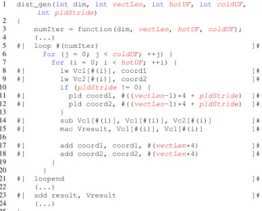
To illustrate some auto-tuning possibilities and how the dynamic language works, Figure 3 presents the deGoal code to auto-tune the euclidean distance implementation, focusing on the main loop of the kernel. This is the code used in the motivational example presented in Section II, and also in the run-time auto-tuning experiments later in this work. Statements between the symbols #[ and ]# are recognized as the dynamic language, which are statically converted to standard C code, calling deGoal library code to generate machine instructions at run time. Other statements are standard C code. An important symbol in the dynamic language is the sign #(): any C expression placed between the parenthesis will be dynamically evaluated, allowing the inlining of run-time constants or immediate values.
The kernel generator (called compilette in the deGoal jargon) description represented in Figure 3 can generate different machine codes, depending on the arguments that it receives. In line 1, the first argument is the dimension, which is specialized in this example. The four following arguments are the auto-tuned parameters:
• Hot loop unrolling factor (hotUF): Unrolls a loop and processes each element with a different register, in order to avoid pipeline stalls.
• Cold loop unrolling factor (coldUF): Unrolls a loop by simply copy-pasting a pattern of code, using fewer registers, but potentially creating pipeline stalls.
• Normalized vector length (vectLen): Defines the length of the vector used to process elements in the loop body, normalized to the SIMD width when generating SIMD instructions (four in the ARM ISA). Longer vectors may benefit code size and speed, because instructions that load multiple registers instructions may be generated.
• Data pre-fetching stride (pldStride): Defines the
stride in bytes used in hint instructions to try to pre-fetch data of the next loop iteration.
Given that the dimension is specialized (run-time constant), we know exactly how many elements are going to be processed
in the main loop. Hence, between the lines 5 and 21, the pair of deGoal instructions loop and loopend can produce three possible results, depending on the dimension and the unrolling factors:
1) No code for the main loop is generated if the dimension is too small. The computation is then performed by a leftover code (not shown in Figure 3).
2) Only the loop body is generated without any branch instruction, if the main loop is completely unrolled. 3) The loop body and a backward branch are generated
if more than one iteration is needed (i.e. the loop is partially unrolled).
The loop body iterates over the coordinates of two points (referenced by coord1 and coord2) to compute the squared euclidean distance. The computation is performed with vectors, but for the sake of paper conciseness, variable allocation is not shown in Figure 3. Briefly, in the loop body, lines 8 and 9 load vectLencoordinates of each point into vectors, lines 14 and 15 compute the difference, squaring and accumulation, and finally outside the loop, line 23 accumulates the partial sums in each vector element of Vresult into result. Between the lines 6 and 20, the loop body is unrolled by mixing three auto-tuning effects, whose parameters are highlighted in Figure 3: the outer for (line 6) simply replicates coldUF times the code pattern in its body, the inner for (line 7) unrolls the loop hotUFtimes by using different registers to process each pair of coordinates, and finally the number of elements processed in the inner loop is set through the vector length vectLen. In the lines 10 to 13, the last auto-tuned parameter affects a data fetching instruction: if pldStride is zero, no pre-fetching instruction is generated, otherwise deGoal generates a hint instruction that tries to pre-fetch the cache line pointed by the address of the last load plus pldStride.
Besides the auto-tuning possibilities, which are explicitly coded with the deGoal language, a set of C functions can be called to configure code generation options. In this work, three code optimizations were studied:
• Instructions scheduling (IS): Reorders instructions to avoid stall cycles and tries to maximize multi-issues.
• Stack minimization (SM): Only uses FP scratch registers to reduce the stack management overhead.
• Vectorization (VE): Generates SIMD instructions to
process vectors.
Most of the explanations presented in this section were given through examples related to the Streamcluster benchmark, but partial evaluation, loop unrolling and data pre-fetching are broadly used compiler optimization techniques that can be employed in almost any kernel-based application.
B. Regeneration decision and space exploration
The regeneration decision takes into account two factors: the regeneration overhead and the achieved speedup since the beginning of the execution. The first one allows to keep the run-time overhead of the tool at acceptable limits if it fails to find better kernel versions. The second factor acts as
1 dist_gen(int dim, int vectLen, int hotUF, int coldUF,
int pldStride) 2 {
3 numIter = function(dim, vectLen, hotUF, coldUF); 4 (...)
5 #[ loop #(numIter) ]#
6 for (j = 0; j < coldUF; ++j) { 7 for (i = 0; i < hotUF; ++i) {
8 #[ lw Vc1[#(i)], coord1 ]# 9 #[ lw Vc2[#(i)], coord2 ]#
10 if(pldStride != 0) {
11 #[ pld coord1, #((vectLen-1)*4 + pldStride) ]# 12 #[ pld coord2, #((vectLen-1)*4 + pldStride) ]#
13 }
14 #[ sub Vc1[#(i)], Vc1[#(i)], Vc2[#(i)] ]# 15 #[ mac Vresult, Vc1[#(i)], Vc1[#(i)] ]# 16
17 #[ add coord1, coord1, #(vectLen*4) ]# 18 #[ add coord2, coord2, #(vectLen*4) ]#
19 }
20 }
21 #[ loopend ]#
22 (...)
23 #[ add result, Vresult ]# 24 (...)
25 }
Fig. 3: Main loop of the deGoal code to auto-tune the euclidean distance kernel in the Streamcluster benchmark. The first function parameter is the specialized dimension, and the other four are the auto-tuned parameters (highlighted variables).
an investment, i.e. allocating more time to explore the tuning space if previously found solutions provided sufficient speedups. Both factors are represented as percentage values, for example limiting the regeneration overhead to 1 % and investing 10 % of gained time to explore new versions.
To estimate the gains, the instrumentation needed in the evaluated functions is simply a variable that increments each time the function is executed. Knowing this information and the measured run-time of each kernel, it is possible to estimate the time gained at any moment. However, given that the reference and the new versions of kernel have their execution times measured only once, the estimated gains may not be accurate if the application has phases with very different behaviors.
Given that the whole space exploration can have hundreds or even thousands of kernel versions, it was divided in two online phases:
• First phase: Explores auto-tuning parameters that have
an impact on the structure of the code, namely, hotUF, coldUFand vectLen, but also the vectorization option (VE). The previous list is also the order of exploration, going from the least switched to the most switched parameter. The initial state of the remaining auto-tuning parameters are determined through pre-profiling.
• Second phase: Fixes the best parameters found in the previous phase and explores the combinatorial choices of remaining code generation options (IS, SM) and pldStride.
In our experiments, the range of hotUF and vectLen were defined by the programmer in a way to avoid running out of registers, but these tasks can be automated and dynamically computed by taking into account the code structure (static)
and the available registers (dynamic information). Compared to coldUF, their ranges are naturally well bounded, providing an acceptable search space size.
The range of coldUF was limited to 64 after a pre-profiling phase, because unrolling loops beyond that limit provided almost no additional speedup.
The last auto-tuned parameter, pldStride, was explored with the values 32 and 64, which are currently the two possible cache line lengths in ARM processors.
Finally, to optimize the space exploration, first the tool searches for kernel implementations that have no leftover code. After exhausting all possibilities, this condition is softened by gradually allowing leftover processing.
C. Kernel evaluation and replacement
The auto-tuning thread wakes up regularly to compute the gains and determine if it is time to regenerate a new function. Each new version is generated in a dynamically allocated code buffer, and then its performance is evaluated. When the new code has a better score than that of the active function, the global function pointer that references the active function is set to point to the new code buffer. In order to evaluate a new kernel version, the input data (i.e., processed data) used in the first and second phases can be either:
• Real input data only: Evaluates new kernel versions
with real data, performing useful work during evaluation, but suffering from measurement oscillations between independent runs. These oscillations can sometimes lead to wrong kernel replacement decisions.
• Training & real input data: Uses training data with
warmed caches in the first phase and real data in the second one. A training input set with warmed caches results in very stable measurements, which ensure good choices for the active function. Since no useful work is performed, using training data is only adapted to kernels that are called sufficient times to consider the overhead of this technique negligible, and to kernels that have no side effect. In the second phase, the usage of real data is mandatory, because the adequacy of pre-fetching instruction depends on the interaction of the real data and code with the target pipeline.
When the evaluation uses real data, the performance of the kernel is obtained by simply averaging the run-times of a pre-determined number of runs.
When the kernel uses a training input data, the measurements are filtered. We took the worst value between the three best values of groups with five measurements. This technique filters unwanted oscillations caused by hardware (fluctuations in the pipeline, caches and performance counters) and software (inter-ruptions). In the studied platforms, stable measurements were observed, with virtually no oscillation between independent runs (in a Cortex-A9, we measured oscillations of less than 1 %).
The decision to replace the active function by a new version is taken by simply comparing the calculated run-times.
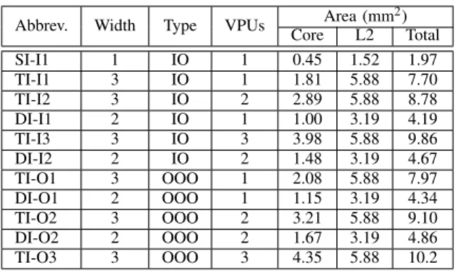
TABLE I: Abbreviation of the simulated core designs and CPU areas
Abbrev. Width Type VPUs Area (mm
2) Core L2 Total SI-I1 1 IO 1 0.45 1.52 1.97 TI-I1 3 IO 1 1.81 5.88 7.70 TI-I2 3 IO 2 2.89 5.88 8.78 DI-I1 2 IO 1 1.00 3.19 4.19 TI-I3 3 IO 3 3.98 5.88 9.86 DI-I2 2 IO 2 1.48 3.19 4.67 TI-O1 3 OOO 1 2.08 5.88 7.97 DI-O1 2 OOO 1 1.15 3.19 4.34 TI-O2 3 OOO 2 3.21 5.88 9.10 DI-O2 2 OOO 2 1.67 3.19 4.86 TI-O3 3 OOO 3 4.35 5.88 10.2
IV. EXPERIMENTAL SETUP
This section presents the experimental setup. First, we detail the hardware and simulation platforms employed in the experiments. Then, the chosen applications for two case studies are described. The kernel run-times and the auto-tuning overhead are measured through performance counters.
Two ARM boards were used in the experiments. One is the Snowball equipped with a dual Cortex-A9 processor [10], an OOO pipeline. The board runs the Linaro 11.11 distribution with a Linux 3.0.0 kernel. The other is the BeagleBoard-xM, which has an IO Cortex-A8 core [11]. The board runs a Linux 3.9.11 kernel with an Ubuntu 11.04 distribution.
A micro-architectural simulation framework [12] was used to simulate 11 different core configurations. It is a modified version of the gem5 [13] and McPAT [14] frameworks, for performance and power/area estimations, respectively. The 11 configurations were obtained by varying the pipeline type (IO and OOO cores) and the number of VPUs (FP/SIMD units) of one-, two- and three-way basic pipelines. Table 1 in [15] shows the main configurations of the simulated cores, and Table I shows the abbreviations used to identify each core design.
Two kernel-based applications were chosen as case studies to evaluate the proposed online auto-tuning approach. To be representative, one benchmark is CPU-bound and the other is memory-bound. In both applications, the evaluated kernels correspond to more than 80 % of execution time. The benchmarks were compiled with gcc 4.9.3 (gcc 4.5.2 for Streamcluster binaries used in the simulations) and the default PARSEC flags (-O3 -fprefetch-loop-arrays among others). The NEON flag (-mfpu=neon) is set to allow all 32 FP registers to be used. The target core is set (-mcpu option) for the real platforms and the ARMv7-A architecture (-march=armv7-a) for binaries used in the simulations. The deGoal library was also compiled for the ARMv7-A architecture, which covers all real and simulated CPUs.
The first kernel is the euclidean distance computation in the Streamcluster benchmark from the PARSEC 3.0 suite. It solves the online clustering problem. Given points in a space, it tries to assign them to nearest centers. The clustering quality is measured by the sum of squared distances. With
high space dimensions, this benchmark is CPU-bound [9]. In the compilette definition, the dimension (run-time constant) is specialized. The simsmall input set is evaluated with the dimensions 32 (original), 64 and 128 (as in the native input set), which are referred as small, medium and large input sets, respectively.
The second kernel is from VIPS, an image processing application. A linear transformation is applied to an image with the Linux command line
vips im_lintra_vec MUL_VEC input.v ADD_VEC output.v. Here, input.v and output.v are images in the VIPS
XYZ format, and MUL_VEC, ADD_VEC are respectively FP vectors of the multiplication and addition factors for each band applied to each pixels in the input image. Given that pixels are loaded and processed only once, it is highly memory-bound. Indeed, the auto-tuned parameters explored in this work are not suitable for a memory-bound kernel. However, this kind of kernel was also evaluated to cover unfavorable situations and show that negligible overheads are obtained. In the compilette description, two run-time constants, the number of bands and the width of the image, are specialized. Three input sets were tested: simsmall (1600 x 1200), simmedium (2336 x 2336) and simlarge (2662 x 5500).
V. EXPERIMENTAL RESULTS
This section presents the experimental results of the proposed online auto-tuning approach in a CPU- and a memory-bound kernels.
A. Real platforms
Table 3 in [15] presents the execution times of all configura-tions studied of the two benchmarks in the real platforms. Figures 4(a) and 4(b) show the speedups obtained in the Streamcluster benchmark. In average, run-time auto-tuning provides speedup factors of 1.12 in the Cortex-A8 and 1.41 in the A9. The speedup sources come mostly from micro-architectural adaption, because even if the reference kernels are statically specialized, they can not provide significant speedups. The online auto-tuning performance is only 4.6 % and 5.8 % away from those of the best statically auto-tuned versions, respectively for the A8 and A9.
Figures 4(c) and 4(d) show the speedups obtained in the VIPS application. Even with the hardware bottleneck being the memory hierarchy, in average the proposed approach can still speed up the execution by factors of 1.10 and 1.04 in the A8 and A9, respectively. Most of the speedups come from SISD versions (SIMD performances almost matched the references), mainly because in the reference code run-time constants are reloaded in each loop iteration, differently from the compilette implementation. In average, online auto-tuning performances are only 6 % away from the best static ones.
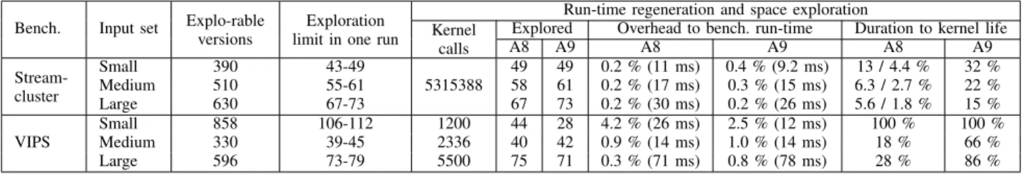
Table II presents the auto-tuning statistics in both platforms. For each benchmark and input set, it shows that between 330 and 858 different kernel configurations could be generated, but in one run this space is limited between 39 and 112 versions, thanks to the proposed two phase exploration (Section III-B).
(a) Streamcluster in Cortex-A8
(b) Streamcluster in Cortex-A9
(c) VIPS in Cortex-A8
(d) VIPS in Cortex-A9
Fig. 4: Speedup of the specialized reference and the auto-tuned applications in the real platforms (normalized to the reference benchmarks).
The online statistics gathered in the experiments are also presented. In most cases, the exploration ends very quickly, specially in Streamcluster, in part because of the investment factor. Only with the small input in VIPS, the auto-tuning did not end during its execution, because it has a large tuning space and VIPS executes during less than 700 ms. The overhead of the run-time approach is negligible, between only 0.2 and 4.2 % of the application run-times were spent to generate and evaluate from 28 to 75 kernel versions.
B. Simulated cores
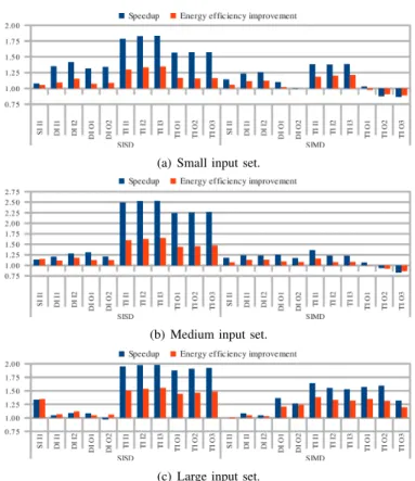
Figure 5 shows the simulated energy and performance of the reference and online auto-tuning versions of the Streamcluster benchmark. In the SISD comparisons, run-time auto-tuning can find kernel implementations with more ILP (Instruction-level parallelism) than the reference code, specially remarkable in the long triple-issue pipelines. The average speedup is 1.58. In the SIMD comparisons, the reference kernel naturally benefits from the parallelism of vectorized code, nonetheless online
(a) Small input set.
(b) Medium input set.
(c) Large input set.
Fig. 5: Speedup and energy efficiency improvement of online auto-tuning over the references codes in the Streamcluster benchmark, simulating the 11 cores. Core abbreviations are listed in Table I.
auto-tuning can provide an average speedup of 1.20. Only 6 of 66 simulations showed worse performance, mostly in big cores that quickly executed the benchmark.
In terms of energy, in general, there is no surprise that pipelines with more resources consume more energy, even if they may be faster. However, there are interesting comparisons between equivalent IO and OOO cores. Here, the term equivalentmeans that cores have similar configurations, except the dynamic scheduling capability.
Still analyzing Streamcluster, when the reference kernels execute in equivalent IO cores, in average their performance is worsened by 16 %, yet being 21 % more energy efficient. On the other hand, online auto-tuning improves those numbers to 6 % and 31 %, respectively. In other words, the online approach can considerably reduce the performance gap between IO and OOO pipelines to only 6 %, and further improve energy efficiency. It is also interesting to compare reference kernels executed in OOO cores to online auto-tuning versions executed in equivalent IO ones. Despite the clear hardware disadvantage, in average the run-time approach can still provide speedups of 1.52 and 1.03 for SISD and SIMD, and improve the energy efficiency by 62 % and 39 %, respectively.
In the simulations of VIPS, the memory-boundedness is even more accentuated, because the benchmark is only called once and then Linux does not have the chance to use disk
TABLE II: Statistics of online auto-tuning in the Cortex-A8 and A9 (SISD / SIMD separated, or average if minor variations).
Bench. Input set Explo-rable versions
Exploration limit in one run
Run-time regeneration and space exploration Kernel
calls
Explored Overhead to bench. run-time Duration to kernel life
A8 A9 A8 A9 A8 A9 Stream-cluster Small 390 43-49 5315388 49 49 0.2 % (11 ms) 0.4 % (9.2 ms) 13 / 4.4 % 32 % Medium 510 55-61 58 61 0.2 % (17 ms) 0.3 % (15 ms) 6.3 / 2.7 % 22 % Large 630 67-73 67 73 0.2 % (30 ms) 0.2 % (26 ms) 5.6 / 1.8 % 15 % VIPS Small 858 106-112 1200 44 28 4.2 % (26 ms) 2.5 % (12 ms) 100 % 100 % Medium 330 39-45 2336 40 42 0.9 % (14 ms) 1.0 % (14 ms) 18 % 66 % Large 596 73-79 5500 75 71 0.3 % (71 ms) 0.8 % (78 ms) 28 % 86 %
blocks cached in RAM. The performance of the proposed approach virtually matched those of the reference kernels. The speedups oscillate between 0.98 and 1.03, and the geometric mean is 1.00. Considering that between 29 and 79 new kernels were generated and evaluated during the benchmark executions, this demonstrates that the proposed technique has negligible overheads if auto-tuning can not find better versions.
In this study, we observed correlations between auto-tuning parameter and pipeline features. The results corroborate the capability of the auto-tuning system to adapt code to different micro-architectures. On the other hand, precise correlations could not be identified, because the best auto-tuning parameters depend on several factors (system load, initial pipeline state, cache behavior, application phases, to name a few), whose behaviors can not be easily modeled in complex systems. Online auto-tuning is a very interesting solution in this scenario.
VI. CONCLUSION
In this paper, we presented an approach to implement run-time auto-tuning kernels in short-running applications. This work advances the state of the art of online auto-tuning. To the best of our knowledge, this work is the first to propose an approach of online auto-tuning that can obtain speedups in short-running kernel-based applications. Our approach can both adapt a kernel implementation to a micro-architecture unknown prior compilation and dynamically explore auto-tuning possibilities that are input-dependent.
We demonstrated through two case studies in real and simulated platforms that the proposed approach can speedup a CPU-bound kernel-based application up to 1.79 and 2.53, respectively, and has negligible run-time overheads when auto-tuning does not provide better kernel versions. In the second application, even if the bottleneck is in the main memory, we observed speedups up to 1.30 in real cores, because of the reduced number of instructions executed in the auto-tuned versions.
Energy consumption is the most constraining factor in current high-performance embedded systems. By simulating the CPU-bound application in 11 different CPUs, we showed that run-time auto-tuning can reduce the performance gap between IO and OOO designs from 16 % (static compilation) to only 6 %. In addition, we demonstrated that online micro-architectural adaption of code to IO pipelines can in average outperform the hand vectorized references run in similar OOO cores. Despite the clear hardware disadvantage, online auto-tuning in IO CPUs
obtained an average speedup of 1.03 and an energy efficiency improvement of 39 % over the SIMD reference in OOO CPUs.
ACKNOWLEDGMENTS
This work has been partially supported by the LabEx PERSYVAL-Lab (ANR-11-LABX-0025-01) funded by the French program Investissement d’avenir.
REFERENCES
[1] M. J. Voss and R. Eigenmann, “ADAPT: Automated de-coupled adaptive program transformation,” in ICPP, 2000.
[2] A. Tiwari and J. K. Hollingsworth, “Online adaptive code generation and tuning,” in IDPDS, 2011.
[3] Y. Chen, S. Fang, L. Eeckhout, O. Temam, and C. Wu, “Iterative optimization for the data center,” in ASPLOS, 2012.
[4] J. Ansel, M. Pacula, Y. L. Wong, C. Chan, M. Olszewski, U.-M. O’Reilly, and S. Amarasinghe, “SiblingRivalry: Online autotuning through local competitions,” in CASES’12.
[5] S. Borkar and A. A. Chien, “The future of microprocessors,” Communi-cations of the ACM, 2011.
[6] J. Ansel, C. Chan, Y. L. Wong, M. Olszewski, Q. Zhao, A. Edelman, and S. Amarasinghe, “PetaBricks: A language and compiler for algorithmic choice,” in PLDI’09, 2009.
[7] H.-P. Charles, D. Courouss´e, V. Lom¨uller, F. A. Endo, and R. Gauguey, “deGoal a tool to embed dynamic code generators into applications,” in Compiler Construction, 2014.
[8] J. M. Cebrian, M. Jahre, and L. Natvig, “Optimized hardware for suboptimal software: The case for SIMD-aware benchmarks,” in 2014 IEEE International Symposium on Performance Analysis of Systems and Software, ser. ISPASS ’14, 2014.
[9] C. Bienia, “Benchmarking modern multiprocessors,” Ph.D. dissertation, Princeton University, January 2011.
[10] Calao Systems, SKY-S9500-ULP-CXX (aka Snowball PDK-SDK) Hard-ware Reference Manual, July 2011, revision 1.0.
[11] BeagleBoard.org, BeagleBoard-xM Rev C System Reference Manual, April 2010, revision 1.0.
[12] F. A. Endo, D. Courouss´e, and H.-P. Charles, “Micro-architectural simulation of in-order and out-of-order ARM microprocessors with gem5,” in SAMOS XIV, 2014.
[13] N. Binkert, B. Beckmann, G. Black, S. K. Reinhardt, A. Saidi, A. Basu, J. Hestness, D. R. Hower, T. Krishna, S. Sardashti, R. Sen, K. Sewell, M. Shoaib, N. Vaish, M. D. Hill, and D. A. Wood, “The gem5 simulator,” SIGARCH Computer Architecture News, vol. 39, 2011.
[14] S. Li, J. H. Ahn, R. D. Strong, J. B. Brockman, D. M. Tullsen, and N. P. Jouppi, “The McPAT framework for multicore and manycore architectures: Simultaneously modeling power, area, and timing,” TACO, 2013.