HAL Id: hal-00451688
https://hal.archives-ouvertes.fr/hal-00451688
Submitted on 29 Jan 2010
HAL is a multi-disciplinary open access
archive for the deposit and dissemination of sci-entific research documents, whether they are pub-lished or not. The documents may come from teaching and research institutions in France or abroad, or from public or private research centers.
L’archive ouverte pluridisciplinaire HAL, est destinée au dépôt et à la diffusion de documents scientifiques de niveau recherche, publiés ou non, émanant des établissements d’enseignement et de recherche français ou étrangers, des laboratoires publics ou privés.
canopies
A. da Silva, C. Sinfort, C. Tinet, Daniel Pierrat, S. Huberson
To cite this version:
A. da Silva, C. Sinfort, C. Tinet, Daniel Pierrat, S. Huberson. A Lagrangian model for spray be-haviour within vine canopies. Journal of Aerosol Science, Elsevier, 2006, 37 (5), p. 658 - p. 674. �10.1016/j.jaerosci.2005.05.016�. �hal-00451688�
A Lagrangian model for spray behaviour within vine canopies
Arthur Da Silva+, Carole Sinfort*, Cyril Tinet*, Daniel Pierrat**, Serge Huberson***+ LRMA – ISAT – BP 31 – 58027 Nevers cedex
*UMR ITAP – Cemagref – BP 5095 – 34033 Montpellier France
**CETIM Nantes, 74 route de la Juonelière- BP 82617 – 44 326 Nantes cedex France ***Université du Havre, 25 rue Philippe Lebon -BP 1123- 76 063 Le Havre cedex France
+Corresponding author. Tel.:+33.499.61.23.34 Fax. +33.499.61.24.36 Email address: [email protected]
Abstract
This work concerns the numerical prediction of pesticide deposits on vine by air assisted sprayers. This numerical model consists in two different parts: the air flow characteristics were obtained through a Navier-Stokes solver in which additional terms have been introduced in order to account for the modification of the flow by the vine foliage. The theoretical form of these terms was derived through an averaging procedure. As a result, the canopy effect was modelled by introducing momentum and turbulence source terms in the Navier-Stokes equations. The constants were identified thanks to experimental data obtained by direct measurements of the air flow speeds through an artificial canopy. The second part of the model consists in simulating the droplet cloud by means of a lagrangian stochastic model. The average motion of the droplets was computed through the use of lagrangian coordinates and the turbulence effect on the droplets was interpreted in term of statistical properties of the droplet cloud. The tractor displacements were accounted for through unsteady boundary conditions. Once the size and the droplets cloud locations have been determined, the deposit was predicted for a vine row of one meter length using an efficiency coefficient obtained from
simulations. Thanks to this approach we were able to quantify the effect of air turbulence on droplet deposition.
Keywords: pesticide droplets, lagrangian model, particle deposition, vine, canopy, collection efficiency
Nomenclature
If not stated, subscript i, j, k stand for the i (respectively j,k)-components of a given entity (Einstein convention)
a: leaf area density [m-1] a1S, a2S, a3S: constants [m-1] b: constant [m-1]
B: body forces
cl: total concentration affected to the l lagrangian particle c(xG,t): particle concentration
Co: drag coefficient for a single leaf [] Can: canopy drag coefficient []
CD: droplet drag coefficient [] Cε1, Cε2, Cµ : constants [] d: droplet diameter [m]
d': maximum deviation of an air molecule [m] dp': maximum deviation of a droplet [m] DT: turbulence diffusivity[m².s-1] E: collection efficiency []
F: resistance body force of the canopy on the air [N.m-3] fg: gravity force per unit mass [N.kg-1]
g: gravitational acceleration [m.s-2] k: turbulent kinetic energy [m2.s-2] L: depth of the canopy [m]
mf: fluid mass corresponding to a droplet volume [kg]
Mi: mass carried by a given injected droplet along its mean trajectory, at the entrance of the ith section [kg]
mp: droplet mass [kg] nG: normal unit vector
p: pressure [N.m-2] pn: shelter factor [] SU, Sk, Sε : source terms t: time [s]
tc: diffusion time of the cloud [s] U: air velocity [m.s-1]
U(y): horizontal air velocity at a given position y [m.s-1]
Ue: mean horizontal air velocity at the entrance of the canopy [m.s-1] Us: mean horizontal air velocity at the output of the canopy [m.s-1] u: component of air velocity [m.s-1]
u': component of the air velocity fluctuation [m.s-1]
l
vG : velocity vector of the l lagrangian particle
v: component of droplet velocity [m.s-1]
v': component of the droplet velocity fluctuation [m.s-1] xG: position vector (components xi)
x: horizontal distance, parallel to the row [m] y: horizontal distance, perpendicular to the row [m] z: vertical distance [m]
αc: correction factor []
Βd, βp: constants δi,j: Kronecker symbol
ε: dissipation rate of energy [m2.s-3]
µ: air viscosity
µT: turbulence dynamical viscosity [kg.m-1.s-1]
νt: turbulence cinematic viscosity [m2.s-1] ρ: air density [kg.m-3]
σ: variance [m]
σT: turbulence Prandlt number []
τp: droplet relaxation time [s]
χl: Position vector of the l lagrangian particle
Introduction
On orchard and bush crops, pesticides are applied with air assisted sprayers. In France, the vineyards consume around 20% of the total amount of commercialized pesticides (~100.000 ton/year) with only 4% of agricultural surface. In these crops, pesticides are sprayed with low volume/hectare rates (50-200 l/ha), consisting of fine sprays (mainly from 25 to 500 micrometers) compared with other applications. This high percentage of small droplets makes them very sensitive to wind resulting in important losses (in some cases more than 50% of the
total, Da Silva et al., 2002). Uneven deposits are also observed (Pergher and Gubiani, 1995) and crop structure and canopy spatial heterogeneity is of great influence on the quality of actual deposit (Gil, 2002).
Vines are cultivated under different plantation forms and using different trailing systems inducing variable distances between trees and between rows (from 1 to 2.50m), variable heights and variable leaf densities. However, canopies during its full developing period more or less form continuous rows standing from the soil up to 1.5m or 2m high, with a depth ranging from 0.5 to 1.5 m and leaf area densities up to 10 m2/m3.
Several authors tried to measure relations between sprayer settlings or spray features and deposits within orchard and vine of various size canopies. Sprayer settings include drive velocity, number, type and size of nozzles, fan velocity, liquid pressure, spray orientation and volume/hectare rates. They were tested for instance by Giles et al. (1989) on peach orchards, Pergher and Gubiani (1995) on vines, Salyani (2000) and Farooq and Landers (2004) on citrus. Important spray characteristics are air and volume flow-rates as well as spray drop size distribution. Test series were setup by Cross et al. (2001a, 2001b, 2003) on apple trees, and much earlier by Randall (1971). Air assistance facilitates spray penetration and shakes the leaves, allowing a better deposit on their back side. Several authors (Reichard et al., 1979; Fox et al., 1985; Brazee et al., 1991) focused on the features of air flow delivered by the sprayers. Many conclusions were obtained but conception of sprayers accounting for all the interacting parameters (atmospheric conditions are also influent factors, mainly for drift considerations) still constitutes a challenging task. Some methods were proposed for adjusting sprays with air flow orientation and distribution irregularities together with canopy shapes and density (Furness et al., 1998; Van de Zande et al., 2001; Vieri and Giorgietti, 2001; Giametta et al., 2002; Pergher et al., 2002) using vertical patternators and/or evaluation of canopy characteristics (Miller et al., 2003).
Field tests are long to set-up and meteorological conditions, tank mixing variability or collection efficiency may affect data homogeneity (Teske and Thistle 2003). Thus, some authors proposed to use numerical simulation as a way to better understand the many phenomena occurring and to improve the calculation of the deposits within canopies. Most advance works in spray modelling were developed for aerial spraying. The AGDISP software (Teske et al., 2003) and its regulatory version, AgDRIFT were developed to predict the behaviour of aircraft releases. They are based on a Lagrangian approach and use original ensemble-averaged turbulence equations avoiding the need of any random component. A Lagrangian approach coupled with stochastic droplet tracking was used for air assisted orchard sprayers by Xu et al. (1998), and by Brown and Sidahmed (2001) as well who provided computations of the horizontal travel distances of droplets released from a forestry airblast sprayer for herbicide applications. In these Lagrangian approaches, only some trajectories were computed, usually one for each class of droplets diameter. The total volume rate of each class was then affected in totality to this representative trajectory.
Raupach et al. (2001a) studied the behaviour of aerial spraying using a Gaussian-plume assumption: the deposit of spray is defined through a conductance [m.s-1] and the concentration of pesticide in the air. The authors stated that the conductance through the vegetation was mainly due to gravitational settling effect and to inertial phenomena. In another paper (Raupach et al., 2001b), the entrapment of particles by windbreaks was considered. It was found to be related to the optical porosity. Finally, Farooq and Salyani (2004) proposed a model for citrus canopies, based on the canopy features of this kind of tree, the amount of deposit on leaves being dependant of collection efficiency of leaves and on the air velocity within the canopy. Compared with these latter models the Lagrangian approach provides more detailed results but, the relatively small number of representative trajectories
which can be computed there introduce the need for an interpolation procedure in order to account for all the droplets.
In this paper the numerical simulation of the behaviour of sprays within vine canopies by means of a Lagrangian approach is proposed. The following simplifying assumption were used : vine sprayers are driven between two canopy walls supposed to be homogeneous in the travel direction and vertical, the outlets are very close to the canopy so the transport between the sprayer and the canopy was not considered, last, due to canopy density, the evaporation within the canopy is supposed to be negligible. The proposed model accounts for the behaviour of the air flow within the canopy, the variation of droplet mean trajectories within this air flow according to their diameters and initial velocities, the behaviour of the spray clouds associated to each trajectory and the rate of input spray entrapped by the leaves. For each of this points, appropriate methods were selected according to vine specifications and the air flow was computed by means of a commercial CFD (Computational Fluid Dynamics) code
1. Modelling air flow within the canopy
Air flow model
A huge amount of work has already been done to analyze air flow behaviour within canopies. Most work was developed for bio-climatology concerns to characterize transfers within the Canopy Sub-Layer (CSL). Most often, the vegetation was supposed to be homogeneous in a horizontal plane and only the vertical dimension was considered.
Interactions between flow and canopy act on two ways: the canopy drag force results in pressure loss in the air flow and air turbulence is modified. It is modelled as a sink term in the
momentum conservation equation and as a source term for the turbulent kinetic energy. Drag force can be split into viscous drag and form drag. Viscous drag is commonly neglected. The influence of canopy structure and variability of drag on momentum was discussed by Bache (1986). The most common expression for the drag force per unit volume is:
U . U . ρ.a.C FG =− n G G [N/m3] (1)
where Cn is the drag coefficient of the canopy, a is the Leaf Area Density, U is the upwind velocity, and ρ the air density.
The turbulence modifications are a production of turbulent kinetic energy (from the mean kinetic energy of the air flow) and a dissipation of the wakes by the elements of vegetation. The representation of the turbulence is an important point of discussion (e.g. Wilson and Shaw, 1977; Katul, 2004). The two equations k-ε model is the most popular in engineering applications and was used in several spray models (Weiner and Parkin, 1993; Zhu et al., 1994; Xu et al., 1998; Brown and Sidhamed, 2001). In this work, the Reynolds averaged equations together with a k-ε model were used. That makes six equations to be solved: the three momentum transport equations (eq. 3), the continuity equation (eq. 2), and two transport equations for k and ε (eq. 5 and 6):
k ε C x ε σ ν x x u x u x u k C C x ε u t ε ε x k σ ν x x u x u x u ν x k u t k ε k C ν and 2 u' k , kδ 3 2 δ x u ν 3 2 x u x u ν u' u' with x ) u' u' (ρ δ x u 3 2 x u x u µ x x p B x u ρu t ρu 0 x ) u (ρ t ρ 2 ε j ε t j j i i j j i µ ε j j j k t j j i i j j i t j j 2 µ t 2 i ij ij l l t i j j i t j i j j i ij l l i j j i i i i j j i i i i 2 1 − ∂ ∂ ∂ ∂ + ∂ ∂ ∂ ∂ + ∂ ∂ = ∂ ∂ + ∂ ∂ − ∂ ∂ ∂ ∂ + ∂ ∂ ∂ ∂ + ∂ ∂ = ∂ ∂ + ∂ ∂ = = + ∂ ∂ + ∂ ∂ + ∂ ∂ − = ∂ ∂ − ∂ ∂ − ∂ ∂ + ∂ ∂ ∂ ∂ + ∂ ∂ − = ∂ ∂ + ∂ ∂ = ∂ ∂ + ∂ ∂ (2) (3) (4) (5) (6) the original publication is available at http://www.elsevier.com - doi:10.1016/j.jaerosci.2005.05.016
These equations are cast into two sets, one for (u, p) and one for (k, ε) which were alternately solved. The computational domain was discretised by means of a finite volume method (Versteeg and Malalasekera, 1995). The numerical scheme was second order in space and time.
Although the k-ε model is usually based on time averaged equations, the dimensional analysis underlying the definition of a turbulent viscosity also holds for space averaging. It was therefore possible to use the same equation supplemented by additional sources terms. An important advantage of this assumption is the possibility to use a commercial CFD solver for the resulting equations: in our case, CFX 4.2 (AEA Technology Engineering Software, Ltd, http://www.aeat.co.uk/) was used. This solver was developed in England more than ten years ago and many applications, both in house at Cemagref and abroad, gave us sufficient confidence in the results, at least for the kind of applications presented hereafter. The quality of the simulations was at least ascertained from the comparison with our experimental results. The computed domain, as shown in Fig. 1 and 2, was a parallelepiped bounded by six rectangular faces and the vine canopy was represented by an embedded sub domain. The canopy was supposed to be homogeneous and was represented by its effects on the air flow. Then, the drag force (eq. 1) was introduced in the momentum conservation equation through a source term, SU:
SU = -Cn.a.U2 (7)
Source terms were also introduced in k and ε equations, respectively Sk and Sε. The expression of Sk is that proposed by Sanz (2003):
.U.k) β .U .a.(β C Sk = n p 3 − d (8)
where βp is the fraction of the mean flow kinetic energy converted to wake-generated k by canopy drag (production of k) and βd (≈1.0 −5.0) is the fraction of k dissipated by interactions with the vegetation. Walklate (1996) suggested that in dense canopies (such in
vines), the production of k and viscous dissipations are small compared with the losses due to crop/flow interactions. Then, taking βd = 1, Sk is simplified to:
Sk = -Cn.a.U.K (9)
Sε is less known and the proposed formulations are mainly based on a standard dimensional analysis (Katul, 2004). The expression retained in our work was:
Sε = -Cn.a.U.ε (10)
consistently to the other source terms expression. Experimental determination of Cn
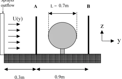
Laboratory experiments were set up using an air-assisted sprayer in front of an artificial canopy, to measure vegetation resistance to airflow. Air velocities were measured with a Phase Droplet Analyser (bi-laser) scanning smoke particles injected at the outlet of the sprayer. Fig. 3 illustrates the organization of the tests. Measurement points were located in two vertical planes, A and B, in front and behind the canopy. The distance between two points was 4 cm in width and 5 cm in height.
Velocities were calculated for an acquisition time of 60s. There were 5 vertical lines of measurements but only the three inside lines (column 2, 3 and 4) were actually represented to avoid side effects. In plane A, mean velocity along z axis, U(yA), was about 7 m/s, whereas in plane B, at the height of the canopy (between 50 and 150 cm), velocity, U(yB), was lower than 2m/s (cf. Fig. 2). Velocity decline is due to momentum absorption by foliage. Stating that the velocity decrease through the canopy is exponential, leads to:
ay) exp(-C U
U(y)= e n (11)
where U(y) is the horizontal velocity at a given position y (see Fig 1) and Ue, the mean horizontal velocity at the entrance of the canopy. Denoting L the depth of the canopy (here L=0.75m), Us, the mean horizontal velocity just behind the canopy, and assuming that Ue is
equal to the mean value of U(yA) (7.2 m/s) and Us to the mean value of U(yB) (≈1.3 m/s), the value of Cn is given by:
s e n U U ln a.L 1 C = (12)
The leaf area density, a, was obtained after gathering all leaves of the artificial plant, by recording images of each leaf with a scanner and then by sizing them using image analysis tools. Its value was 7 m-1, giving then:
Cn ≈ 0.3
This value is in agreement with those found in literature, where 0.1 < Cn < 0.5. The value 0.5 corresponds to a single leaf perpendicular to the flow. The 0.3 value obtained is due to a shelter effect, caused by the surrounding leaves. The shelter factor, pn, was defined by Raupach and Thom (1981) as:
pn = Co (U) / Cn (U) (13)
where Co is the friction coefficient for a single leaf, Cn the effective friction coefficient and U, the air velocity. In the case of the artificial plant, applying equation (13) gives pn equal to 1.7.
Model setting
The computed domain is shown in Fig. 2. It was uniformly covered with cubic cells which sides correspond to a 5 cm actual length. The air flow and, in the next stage, the droplets are injected in a plane which will be referred to as the inlet boundary. Boundary conditions were defined for the six rectangular faces bounding the domain. Because of the airflow generation process, constant pressure boundary conditions were used for all the bounding faces except for the inlet boundary and for the ground face where no-slip boundary conditions were used. The inlet boundary, shown on Fig. 1 and 2, is 3 m long and 0.9 m high; it was discretised into 1080 cells (60×18).
Results
The comparison of simulations and experience (Fig. 4) shows that, on the whole, computed velocities satisfactorily fit measured ones. Hence, the used resistance force gave a good approximation of the canopy effect on air flow.
2. Simulation of mean trajectories
Lagrangian model
Assuming, there is no interaction between the droplets and the airflow, droplet transport is governed by equation (14):
(
)
(
)
l l i p f p i i p 2 D i v dt χ d g m m m v u v u ρ 8m πd C dt dv G G = − + − − = (14)where vi is the i-component of droplet velocity, CD the droplet drag coefficient (computed from the Reynolds number of the droplet.), mp and d the droplet mass and diameter, ui the
component of air velocity, mf the fluid mass corresponding to a droplet volume and gi the i-component of gravitational acceleration. χGl stands for the position vector of the l droplet, and
l
vG for its velocity vector.
The turbulence effect on the trajectories can be dealt with in many different ways. General CFD codes as CFX or Fluent (Fluent Inc., Lebanon, N.H.) describe the effect of turbulence dissipation by stochastic droplet tracking assuming that the air fluctuating velocities obey a Gaussian probability function (as described in Reichard et al., 1992). Another method is to use random-walk models where the temporal fluctuation of the air velocity is determined by means of a Markov process (described for instance in Miller and Hadfield, 1989; Mokeba et al., 1997 or Xu et al., 1998). The AGDISP model is based on a spectral representation of the fluctuating velocity (Teske et al., 2003). The present work was based on the computation of averaged trajectories for a set of representative droplets. At this stage, only the mean flow was accounted for. Each droplet was assumed to correctly represent the average motion of a set of similar droplets gathered in a “droplet cloud”. The air velocity fluctuations were accounted for through the expansion of these droplet clouds along the averaged trajectories. As a result, the droplet concentration associated to the l lagrangian particle is expressed as the Gaussian function:
(
)
∏
= − − = 3 1 i 2i 2 i l, i i l (t) σ (t)) χ (x exp (t) πσ 2 c t) , x c(G (15)The equation governing σi(t) is further described in the next section.
Model setting
Droplets, assisted by air flow, were injected from the inlet boundary, at a 0.3 m distance from foliage. To represent the horizontal displacement of the sprayer along the vine row, the airflow starts abruptly according to a Heaviside function, so that it can be considered to be a
vertical band moving from the left to the right, according tothe tractor displacement direction (x-direction). The band width can be regulated in a Fortran routine associated with the numerical simulation.
Droplet distributions were measured with the Phase Doppler Analyser and were sorted within five diameter classes. The input spray was represented by 4 injection points, in a same vertical axis. At each injection point, a droplet of each diameter class was released with the flowrate of the entire class. The droplet input velocity was set to the mean air velocity input. As far as the droplets are concerned, they are assisted by the airflow. At a given time step, 20 droplets of the 5 different diameter classes are ejected from the 4 vertical positions corresponding to the 4 outlets. In the following step, the injection position moved forward, in the x direction (cf. Fig. 5). The injection of droplets was set to occur during sixty two-second steps. This time corresponds to the tractor moving at a speed of 1.5 m/s in front of a 3m vine row. To summarize, 20 × 60 = 1200 mean trajectories were computed.
3. Computation of cloud expansion
Expansion model
The 1200 mean trajectories are not representative of all individual droplets ejected from the sprayer. The individual droplets are much more numerous. Therefore, these many droplets were cast into 1200 possibly overlapping clouds surrounding the 1200 previous particles. The individual motion of a droplet belonging to one such given cloud was assumed to be defined as the addition of the corresponding mean motion plus a fluctuation. These fluctuations were expected to be conveniently modelled by independent Brownian motions whose diffusion can be related to some turbulence quantification. With this hypothesis, for a given diameter, the position of one set of droplets around their mean trajectory was supposed to follow a Gaussian
distribution whose variance is a function of turbulent parameters of the k-ε model. Turbulence viscosity is defined as:
ε ν µ 2 k C T = (16)
where Cµ = 0.09 is a constant parameter. Turbulence diffusivity has the following form:
T T T D
σ
ν
= (17)where σT is the turbulence Prandlt number.
To respect energy conservation, a factor 1/3 appears for each velocity component. It means that for i-component, turbulence diffusivity becomes:
T T T i T 31D 3σ D = =
ν
(18)Following the Brownian motion model, the expression of variance is given by:
c T 2 µ c T 2 i 3σ ε t k C 2 t D 2 σ i = = (19)
where tc is the diffusion time of the cloud. Hence, the variance of the cloud is function of k and ε and is time dependant.
Integration of turbulence parameters in space and time
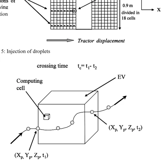
The vine domain was divided in 240 elementary representative volumes (EV). An EV is a cube, which sides are 30cm long and it is considered as a homogeneous domain. It then contains 63 (= 216) cells. A post-process was developed to compute the variance of the cloud for a given mean trajectory and for every crossed EV. The diffusion time of the cloud, tc, is the crossing time of the EV. It depends on droplet inertia and on the distance travelled within the EV. Turbulence energy and dissipation rate were integrated within all computing cells contained in the EV during this time tc (cf. Fig. 6).
Correction factor including droplet relaxation time
The variance previously defined for the expansion of the cloud only corresponds to the expansion of air molecules. Brownian motion is indeed only of value for particles smaller than one micron. The variance of the expansion of the cloud for bigger particles must include a correction factor, αc, relating the dispersion of air molecules and droplets, by taking into account the relaxation time of the droplets.
If ∆σi is the air molecules variance increase (for i-component) while crossing an EV, and ∆σPi the corresponding actual expansion of a droplet cloud, the correction factor will be:
1 ∆σ ∆σ α i Pi c = < (20)
αc tends to 0 when droplet diameter becomes very big, and αc ≈ 1 for very small droplets.
Calculation of αc follows:
If ui' is the i-component of the air velocity fluctuation, it was assumed that the corresponding droplet velocity fluctuation followed an exponential law defined as:
(
t/τp)
i i'(t) u '1 e
v = − −
, (21)
where τp is the droplet relaxation time.
In a given EV, the maximum deviation of a droplet, during a crossing time, tc, is:
dt ' v ' d c t 0 i i p =
∫
, (22)while the maximum deviation of an air molecule is:
c i i' u t'
d = . (23)
Then, it can be considered that αc is given by:
' d ' d α i Pi c = (24)
In this work, the relaxation time, τp, was estimated for each class of droplet diameter without considering non-linear forces. A cloud that increases while crossing the vegetation (as illustrated in Fig. 7, for the z-component) was associated to each mean trajectory.
4. Particle deposition
Impact model
As the canopy was represented as a homogeneous domain, it was necessary to determine the part of the spray retained by the leaves. Most models compute deposits as proportional to a “collection efficiency” (or “impaction efficiency” or “probability collection”) which use and definition is variable but which always accounts for the inertial behaviour of the droplets and, in some cases, for the entrapment behaviour at the leaf level (Xu et al. 1998; Raupach et al., 2001b; Teske et al., 2003; Farooq and Salyani, 2004). The description of the expression of this coefficient will not be considered here.
The 240 EV were grouped in 5 vertical sections in depth direction (y). The mean trajectories cross successively the 5 sections and thus, five EV, assuming that the droplets never return backwards. In each EV, the deposit was computed as the mass carried by the
( ) ( ) z d e * σ 2π 1 x d e * σ 2π 1 V 2 P 2 2 P 2 Zc ∆z/2 2σ1* z Z ∆z/2 Zc X x * σ 2 1 ∆x/2 Xc ∆x/2 Xc frac − − + − − − + −
∫
∫
=fraction of each cloud (around each mean trajectory) crossing the EV, corrected by a collection efficiency, denoted E. For every crossed EV, the deposit is then given by the relation: V n . V M E V Dep frac i G G G × × × = (25)
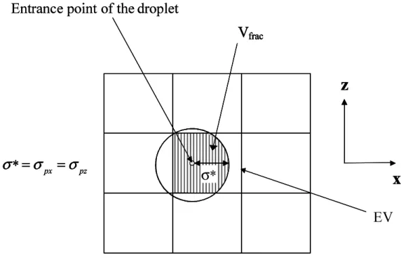
Mi is the mass carried by a given injected droplet along its mean trajectory, at the entrance of the ith section. At the entrance of the canopy, M1 is computed from the mass flow rate of the sprayer. At the ith section, Mi = Mi-1 - Depi-1., where Depi-1 stands for the sum of the deposits in all the EV's of the section i-1. nGis the normal unit vector of the entrance plane in any EV. E was obtained from repeated simulations with injections in front of squared vertical leaves, depending on the droplet diameter and velocity, on a shelter factor and on the leaf area density. Vfrac is the fraction of the cloud that enters a given EV as shown in Fig. 8. The standard deviation of the cloud σ* is the same in both x and z direction (σ* = σx = σz). Then, writing the Brownian expression of the cloud within the limits of an EV gives:
(26)
where xc and zc are the co-ordinates of the centre of the EV, ∆x and ∆z the size of the EV, xp and zp, the co-ordinates of the droplet at the EV entrance.
Vfrac is computed for all the EV's of a same vertical section crossed by any part of the cloud allowing then to obtain the deposit within each EV. The deposits are ultimately tallied in every EV for all injected droplets.
Example of results
Trajectories were computed for 3 meters of vegetation length. Only a one meter long central section was kept in order to avoid boundary effects. The LAD was 7 m-1 for all the EV's and the shelter factor was pn=1.82. The deposits accumulated along this meter of vine length show an exponential decrease, as for a scalar, S, crossing a canopy (cf. Fig. 9):
y.b 0 e
S
S= × − (27)
Walklate (1996) suggested that b = a1S + a2S + a3S where a2S accounts for the vegetation, a1S, for the expansion of the spray, and a3S, for leaf movement. In our case, a2S is known (a2S = Cn a), and a3S is neglected. As a result, the model can be used to evaluate the turbulence effect on the deposit yielding:
a1S = b - a2S (28)
Conclusion
The approach proposed here allows us to predict the effect of physical parameters (droplet diameter, air and droplet velocities, air turbulence at the sprayer output, flow rate, leaf area density) on spray efficiency within the canopy. The model doesn’t take into account the transport between the sprayer and the canopy and focuses on the behaviour inside the canopy. In row per row applications, this representation is expected to be sufficient to describe the entire process. In the general case, with airblast or pneumatic sprayers, when vines are sprayed every two rows (or more), an important amount of spray can be lost in the air and transport and evaporation outside the canopy must be considered.
The model is based on the representation of the canopy through a resistance force as well as modifications of turbulence parameters. Then, the spray is represented by a selected number of droplet clouds. The history of each cloud is derived from the individual trajectory
of one representative droplet and a Brownian motion. It was also assumed that the droplets of one particular cloud have approximately the same diameter and carry an equivalent mass of liquid. One key element is the model for the expansion of droplet clouds around the mean trajectories. This expansion is obtained through the relation between the Brownian motion parameters and the turbulence and droplets dynamic. The different droplet sizes were accounted for by mean of a relaxation time. The canopy is divided into elementary volumes with variable leaf area densities. The deposits are obtained for each of these elementary volumes. The computation of the deposit relies on a collection efficiency factor which was obtained by separate simulations. This collection efficiency could be used to analyze the role of the influencing parameters and to improve the pre-existing relations. A further work will focus on this point.
One particular advantage of our model is the relation which was clearly established between the different physical phenomena, their mathematical representation using physical parameters and their introduction into the final deposit estimate. The next target will be to use this model to improve and optimize air assistance in sprayers.
References
Bache, D.H. (1986), 'Momentum transfer to plant canopies: influence of structure and variable drag',
Atmospheric Environment 20, 1369-1378.
Brazee, R.D.; Reichard, D.L.; Bukovac, M.J. & Fox, R.D. (1991), 'A partitioned energy transfer model
for spray impaction on plants',
Journal of Agricultural Engineering Research 50(1), 11-24.Brown, R.B. & Sidhamed, M.M. (2001), 'Simulation of spray dispersal and deposition from a forest
airblast sprayer -
Part II: Droplet trajectory model',
Transactions of the ASAE 44(1), 11-17.Cross, J.V.; Walklate, P.J.; Murray, R.A. & Richardson, G.M. (2001a), 'Spray deposits and losses in
different sized apple trees from an axial fan orchard sprayer: 1. Effects of spray liquid flow rate',
Crop Protection 20(1), 13-30.
Cross, J.V.; Walklate, P.J.; Murray, R.A. & Richardson, G.M. (2001b), 'Spray deposits and losses in different sized apple t
rees from an axial fan orchard sprayer: 2. Effects of spray quality',
Crop Protection 20(4), 333-343.Cross, J.V.; Walklate, P.J.; Murray, R.A. & Richardson, G.M. (2003), 'Spray deposits and losses in
different sized apple trees from an axial fan orchard sprayer: 3. Effects of air volumetric flow rate',
Crop Protection 22(2), 381-394.
DaSilva, A.; Sinfort, C.; Bonicelli, B.; Voltz, M. & Huberson, S. (2002), 'Spray penetration within vine canopies at different vegetative stages', Aspects of Applied Biology 66, 331-339.
Farooq, M. & Landers, A.J. (2004),'Interactive effects of air, liquid and canopies on spray patterns of axial-
flow patterns' Paper 041001, ASAE, Fermont Chateau Laurier .
Farooq, M. & Salyani, M. (2004), 'Modelling of spray penetration and deposition on citrus tree canopies', Transactions of the ASAE 47(3), 619-627.
Fox, R.D.; Brazee, R.D. & Reichard, D.L. (1985), 'A model study of the effect of wind on air sprayer
jets', Transactions of the ASAE 28(1), 83-88.
Furness, G.O.; Magarey, P.A.; Miller, P.H. & Drew, H.J. (1998), 'Fruit tree and vine sprayer
calibration based on canopy size and length of row: unit canopy row method',
Crop Protection17(8), 639-644.
Giametta, G.; Giametta, F. & Caracciolo, G. (2002),'Optimization of plant protection treatment in a
vineyard' Paper 021097, ASAE International Meeting/CIGR XVth World Congress, Chicago, Illinois.
Gil, E. (2002),'Crop adapted spraying in vineyard. Leaf area distribution (crop profile) and uniformity
of deposition (CV) as tools to evaluate the quality of applications' Paper 02-PM-014, AGENG, Budapest, Hungary.
Giles, D.K.; Delwiche, M.J. & Dodd, R.B. (1989), 'Spatial distribution of spray deposition from an air
-carrier sprayer', Transactions of the ASAE 32(3), 807-811.Katul, G.G. (2004), 'One an
d two equations models for canopy turbulence',
Boundary-LayerMeteorology 113(1), 81-109.
Miller, P.C.H. & Hadfield, D.J. (1989),’A simulation model of the spray drift from hydraulic nozzles’,
Journal of Agricultural Engineering Research 42, 135-147
Miller, P.C.H.; Scotford, I.M. & Walklate, P.J. (2003),'Characterizing crop canopies to provide a basis
for improved pesticide application' Paper 031094, ASAE Annual International Meeting, Las Vegas.
Pergher, G.; Balsari, P.; Cerruto, E. & Vieri, M. (2002), 'The relationship between vertical spray
patterns from air
-assisted sprayers and deposits in vine canopies', Aspects of Applied Biology 66, 323-330.Pergher, G. & Gubiani, R. (1995), 'The effect of spray application rate and airflow rate on foliar deposition in a hedgerow vineyard', Journal of Agricultural Engineering Research 61, 205-216.
Randall, J.M. (1971), 'The relationships between air volume and pressure on spray distribution in fruit
trees', Journal of Agricultural Engineering Research 16(1), 1-31.
Raup
ach, M.R.; Briggs, P.; Ahmad, N. & Edge, V.E. (2001), 'Endosulfan transport II: Modeling
airborne dispersal and deposition by spray and vapor', Journal of Environmental Quality 30, 729-740.Raupach, M.R. & Thom, A.S. (1981), 'Turbulence in and above plant canopies',
Annual Review of Fluid Mechanics 13, 97-129.Raupach, M.R.; Woods, N.; Dorr, G.; Leys, J.F. & Cleugh, H.A. (2001), 'The entrapment of particles
by windbreaks', Atmospheric Environment 8, 1-11.
Reichard, D.L.; Fox, R.D.; Brazee, R.D. & Hall, F.R. (1979), 'Air velocities delivered by orchard air sprayers', Transactions of the ASAE 22(1), 69-74, 80.
Reichard, D.L.; Zhu, H.; Fox, R.D.& Brazee, R.D. (1992), ‘Wind tunne validation of a c
omputer
program to model spray drift’,
Transactions of the ASAE 35(3), 755-758Salyani, M. (2000), 'Optimization of deposition efficiency for airblast sprayers',
Transactions of the ASAE 43(2), 247-253.Sanz, C. (2003), 'A note on k-
epsilon modelling of ve
getation canopy air-flow', Boundary LayerMeteorology 108, 191-197.
Teske, M.E.; Thistle, H.W. & Ice, G.G. (2003), 'Technical advances in modelling aerially applied
the original publication is available at http://www.elsevier.com - doi:10.1016/j.jaerosci.2005.05.016sprays', Transactions of the ASAE 46(4), 985-996.
Teske, M.E. & Thistle, H.W. (2003), 'Release height and far-
field limits of lagrangian aerial spray
models',
Transactions of the ASAE 46(4), 977-983.Van de Zande, J.C.; Porskamp, H.A.J. & Michielsen, J.M.G.P. (2001), 'Effect of the spray distribution
set-up of a cross-flow fan orchard sprayer on the spray deposition in a flat surface and in a tree',
Parasitica 57(1--2--3), 87-97.
Versteeg, H.K. & Malalasekera, W., (1995), An introduction to Computational Fluid Dynamics. The
finite volume method. Prentice Hall ed. 257 p.
Vieri, M. & Giorgetti, R.
(2001), 'Results of the comparative efficiency distribution trials on two
sprayers (conventional GEO-diffuser and OKTOPUS-spraying modules) using different settings',
Advances in Horticultural Sciences 15(1-4), 112-120.
Wilson, N.R. & Shaw, R.H. (1977), 'A
higher order closure model for canopy flow',
Journal of Applied Meteorology 16(11), 1197-1205.Xu, X.G.; Walklate, P.J.; Rigby, S.G. & Richardson, G.M. (1998), 'Stochastic modelling of turbulent
spray dispersion in the near-field of orchard sprayers', Journal of Wind Engineering and Industrial
Aerodynamics 74-76, 295-304.
Zhu, H.; Reichard, D.L.; Fox, R.D.; Brazee, R.D. & Ozkan, H.E. (1994), 'Simulation of drift of
discrete sizes of water droplets from field sprayers',
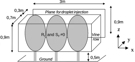
Transactions of the ASAE 37(5), 1401-1407.Figure 1 – Dimensions of the modelled part of the vine row
Figure 2 – The whole computational domain
0,9m 0,9m 0,5m 3m 0,3m 0,7m Ground Vine row Plane for droplet injection
z
y
x
Rf and SF≠0 0,9m 0,9m 0,5m 3m 0,3m 0,7m Ground Vine row Plane for droplet injectionz
y
x
z
y
x
Rf and SF≠0 boundaries Vine region with source terms Pressureboundaries
3m Ground : wall boundaries
Pressure Vine region with terms Pressure
boundaries
3m Ground : wall boundaries
Pressure
z
y
x
0.9 m
Grid for droplet injection
boundaries Vine region with source terms Pressure
boundaries
3m Ground : wall boundaries
Pressure Vine region with terms Pressure
boundaries
3m Ground : wall boundaries
Pressure
z
y
x
z
y
x
0.9 mGrid for droplet injection
0.7m
0.9m
0.3m
B Ay
z
L = U(y) Sprayer outflowFigure 3 – Measurement of air flow velocities in front of (plane A, y = yA), and behind (plane B, y = yB), an artificial plant 0.00 0.50 1.00 1.50 2.00 0.00 1.00 2.00 3.00 4.00 5.00 6.00 7.00 8.00 9.00
Plane B - Measure Plane A - Measure Plane B - Simulation Plane A - Simulation
Figure 4 – Comparison between experimental and calculated velocities in front of and behind an artificial canopy.
Figure 5: Injection of droplets
Figure 6: Droplet crossing an EV
1 point of throwing 5 droplet classes • • • • • • • • • • • • • • • • • • • • • • • • • • • • • • • • Tractor displacement 3 m divided in 60 cells 0.9 m Emission point M 4 vertical positions of throwing
x
z
divided in 18 cells 1 point of throwing 5 droplet classes • • • • • • • • • • • • • • • • • • • • • • • • • • • • • • • • Tractor displacement 3 m divided in 60 cells 0.9 m Emission point M 4 vertical positions of • • • • • • • • • • • • • • • • • • • • • • • • • • • • • • • • • • • • • • • • • • • • • • • • • • • • • •• • • • • • • • • • • • • • • • • • • • • • • • • • • • • • • • • • • • • • • • • • • • • • • • • • • • • • • • • • • • • • • • • • • • • • • • • • • • • • • • • • • • • • • • • • • • • • • • • • • • • • • • • • • • • • • • • • • • •• • • • • • • • • • • Tractor displacement 3 m divided in 60 cells 0.9 m Emission point M 4 vertical positions ofx
z
divided in 18 cells injection injection 1 point of throwing 5 droplet classes • • • • • • • • • • • • • • • • • • • • • • • • • • • • • • • • Tractor displacement 3 m divided in 60 cells 0.9 m Emission point M 4 vertical positions of throwingx
z
divided in 18 cells 1 point of throwing 5 droplet classes • • • • • • • • • • • • • • • • • • • • • • • • • • • • • • • • Tractor displacement 3 m divided in 60 cells 0.9 m Emission point M 4 vertical positions of • • • • • • • • • • • • • • • • • • • • • • • • • • • • • • • • • • • • • • • • • • • • • • • • • • • • • •• • • • • • • • • • • • • • • • • • • • • • • • • • • • • • • • • • • • • • • • • • • • • • • • • • • • • • • • • • • • • • • • • • • • • • • • • • • • • • • • • • • • • • • • • • • • • • • • • • • • • • • • • • • • • • • • • • • • •• • • • • • • • • • • Tractor displacement 3 m divided in 60 cells 0.9 m Emission point M 4 vertical positions ofx
z
divided in 18 cells injection injection Computing cell EV (Xp, Yp, Zp, t1) (Xp, Yp, Zp, t2) crossing time tc= t1- t2 Computing cell EV (Xp, Yp, Zp, t1) (Xp, Yp, Zp, t2) crossing time tc= t1- t2 Computing cell EV (Xp, Yp, Zp, t1) (Xp, Yp, Zp, t2) crossing time tc= t1- t2 Computing cell EV (Xp, Yp, Zp, t1) (Xp, Yp, Zp, t2) crossing time tc= t1- t2Figure 7: Droplet cloud expansion (for z component) while crossing the vegetation divided into several EV. σp: variance of the droplet cloud
Figure 8: Fraction of the cloud entering a given EV, used for the computation of the coefficient Vfrac σpz(EVn+1) z σpz(EVn) n n+1 σpz(EV1) 30 cm σpz(0) = 0
Injection plane : 1200 droplets = 1200 mean trajectories
y Mean trajectory σpz(EVn+1) z σpz(EVn) n n+1 σpz(EV1) 30 cm σpz(0) = 0
Injection plane : 1200 droplets = 1200 mean trajectories
y Mean trajectory
V
fracσ*
z
x
V
fracσ*
V
fracσ*
z
x
EV
pz pxσ
σ
σ
*
=
=
Entrance point of the droplet
V
fracσ*
z
x
V
fracσ*
V
fracσ*
z
x
EV
pz pxσ
σ
σ
*
=
σ
px=
σ
pzσ
*
=
=
Entrance point of the droplet
Figure 9: Modelled accumulated deposit in the canopy for a 1 metre vine row y = 8166.5e -3.8169x R2= 0.996 0 1000 2000 3000 4000 5000 6000 7000 8000 9000 10000 0 0.2 0.4 0.6 0.8 1 1.2 canopy depth (m) Cu m u la te d d e p o s it (m g ) y = 8166.5e -3.8169x R2= 0.996 0 1000 2000 3000 4000 5000 6000 7000 8000 9000 10000 0 0.2 0.4 0.6 0.8 1 1.2 canopy depth (m) Cu m u la te d d e p o s it (m g )