HAL Id: hal-02401208
https://hal.archives-ouvertes.fr/hal-02401208
Submitted on 12 Dec 2019HAL is a multi-disciplinary open access archive for the deposit and dissemination of sci-entific research documents, whether they are pub-lished or not. The documents may come from teaching and research institutions in France or abroad, or from public or private research centers.
L’archive ouverte pluridisciplinaire HAL, est destinée au dépôt et à la diffusion de documents scientifiques de niveau recherche, publiés ou non, émanant des établissements d’enseignement et de recherche français ou étrangers, des laboratoires publics ou privés.
Fluid-structure interaction in two-phase flow using a
discrete forcing method
J. Laviéville, N. Mérigoux, W Benguigui
To cite this version:
J. Laviéville, N. Mérigoux, W Benguigui. Fluid-structure interaction in two-phase flow using a discrete forcing method. International Journal for Numerical Methods in Fluids, Wiley, 2019, �10.1002/fld.4753�. �hal-02401208�
DOI: xxx/xxxx
ARTICLE TYPE
Fluid-structure interaction in two-phase flow using a discrete
forcing method
W. Benguigui
1,2| J. Laviéville
1| N. Merigoux
11Fluid Mechanics, Energy and Environment Department, EDF R&D, 6 Quai Watier, 78400 Chatou, France
2, IMSIA, UMR EDF/CNRS/CEA/ENSTA 9219, Université Paris-Saclay, 91762 Palaiseau, France
Correspondence
Email: [email protected]
Summary
The numerical simulation of interaction between structures and two-phase flows is a major concern for many industrial applications. Using a discrete forcing method1
(implemented in a multi-phase CFD code based on a two-fluid approach) to track the solid motion in two-phase flow, an iterative fluid-structure coupling is developed to allow free-motion of multiple solids (with any kind of geometry) due to two-phase fluid forces. As the fluid-structure interface is located thanks to a time and space dependent porosity on a cartesian grid, the fluid force computation is accommodated to the interface tracking method. A Newmark algorithm is used to estimate the solid motion. The iterative coupling is addressed in detail going from the algorithm to the determination of its convergence parameter. Three application cases are proposed to validate the method from motion under a single- to a two-phase flow.
KEYWORDS:
Fluid-structure interaction, Two-phase flow, Immersed Boundary, CFD
1
INTRODUCTION
In industrial applications such as nuclear, petroleum industry or naval engineering, mobile solid bodies in two-phase flows are a major concern as they might be involved in different possible damages. Consequently, several points of view can be considered to investigate them through experiments or numerical simulations. For the purpose of this work, numerical simulation is considered. In the context of strongly coupled physics like fluid-elastic instability for example, the coupling between fluid and structure solvers is a complex topic. Methods to solve fluid-structure interaction problems are classified into two groups: the monolithic method and the partitioned method. The coupling between a fluid and a structure is located at the interface between each domain. Interfaces have to remain in contact, this is illustrated by two conditions :
• fluid and structure interfaces are displaced with the same velocity:
• interface loads from structure and fluid are equal.
In order to ensure these conditions, monolithic and partitioned methods are suitable.
With the monolithic approach, fluid and solid subdomains do not have distinction in their space and time discretizations2,3.
Based on a joint algorithm, subdomains are computed simultaneously. Despite the good behavior of these algorithm, it requires the development of a code since fluid and solid solvers are often different and difficult to combine. Consequently, the use of partitioned algorithm is more frequent.
In mirror, the partitioned method solves distinctly fluid and solid systems. Physical domains are often different but exchange data through the fluid-structure interface. This flexibility in the choice of the discretization of each subdomain is the main
advantage. Complex solvers developed at first for each subproblem might be utilized with the partitioned approach. Partitioned approach is classified into two groups4,5,6,7,8:
• Explicit coupling (weakly coupled): subproblems are solved only once, consequently it is low time-consuming coupling. The fluid domain is first solved; then, based on the updated fluid load, solid equations are solved. However, the interface displacement is approximated which may generate energy at the interface leading to unstable solutions. The density ratio between solid and fluid is a key point in this instability called added mass effect.
• Iterative implicit coupling (strongly coupled): by utilizing sub-iterations to solve solid and fluid systems, interface con-ditions are respected. In fact, the explicit coupling is used at each sub-iteration, step by step the wall force and the displacement are computed. Once convergence is reached, it goes to the next iteration. This approach looks like the mono-lithic approach. These methods have the inconvenient to be slow. Different methods have been developed for years to accelerate this procedure but are not detailed in the present work9,10.
There are consequently multiple ways to perform fluid-structure coupling. In our case, the partitioned approach is required since we already have a fluid solver. Having strongly coupled problem of tube vibration induced by flow, the choice has been made to use an iterative implicit coupling which is presented in the following section. Because of the specific character of the interface tracking method used in the present work1, the force computation is detailed. Then, the displacement prediction algorithm from
Newmark is presented. Finally, the iterative fluid-structure coupling using the Time and Space Dependent Porosity method is detailed. The coupling is then validated on a very simple case to adjust its parameters. A single- and a two-phase flow cases are realized and compared to experimental data.
2
NUMERICAL MODELING
2.1
Two-phase flow modeling
The present work involves a CFD code dedicated to multiphase flows and based on the two-fluid (extended to 𝑛) approach. NEPTUNE_CFD code developed in the framework of the NEPTUNE project11(funded by EDF, CEA, Framatome and IRSN)
is a finite-volume code with a collocated arrangement for all variables. The data structure is totally face-based, which allows the use of arbitrary shaped cells (tetrahedra, hexahedra, prisms, pyramids, ...). Using a pressure correction approach12, it is able to
simulate multiphase flows by solving a set of three balance equations for each field. These balance equations are deduced from volumetric averaging of local instantaneous balance equations where the 𝑘-phase volumetric fraction is written 𝛼𝑘. In multiphase flow, one property of the 𝑘-phase volumetric fractions is:
𝑁
∑
𝑘=1
𝛼𝑘= 1 (1)
with 𝑁 the number of fluid phases included into the fluid domain.
Fields can represent different kinds of multiphase flows. The present work is focusing on liquid-gas flows only and restricted to adiabatic cases, simplifying the system to the mass and momentum balance equations for each phase 𝑘:
𝜕(𝛼𝑘𝜌𝑘) 𝜕𝑡 + ⃗∇⋅ (𝛼𝑘𝜌𝑘 ⃗ 𝑈𝑘) = 0 𝜕 ( 𝛼𝑘𝜌𝑘𝑈⃗𝑘 ) 𝜕𝑡 + ⃗∇⋅ ( 𝛼𝑘𝜌𝑘𝑈⃗𝑘𝑈⃗𝑘)= −𝛼𝑘∇𝑃 + 𝛼⃗ 𝑘𝜌𝑘𝑔⃗+ ⃗∇⋅ 𝜏𝑘+ 𝑁 ∑ 𝑝=1 𝑝≠𝑘 ⃗ 𝑀𝑝→𝑘 (2)
where 𝛼, 𝜌, ⃗𝑈, 𝑃 , 𝜏, ⃗𝑔and ⃗𝑀are respectively the volume fraction, the density, the velocity, the pressure, the Reynolds-stress tensor, the gravity and the momentum transfer to the phase 𝑘. Depending on the forms of the same physical components, i.e.: a continuous or dispersed field, the interfacial momentum transfers of each phase are defined. Different approaches are consequently possible depending on the two-phase flow regime. For a bubbly flow, a dispersed approach for the gas field is more appropriate13. However, for stratified or slug flow, a Large Interface approach seems to be more suitable14. To deal with multi-regime flow, where small and large bubbles are present, both models using respectively two and three fields are implemented: the Generalized Large Interface To Dispersed approach15and the Multi-Field approach16.
2.2
Fluid-structure interface tracking method
The aim of discrete forcing methods is to strictly ensure the conservation laws at the close vicinity of the interface. The idea is to reshape the cells crossed by the interface and to build specific schemes inside them. The interface is approximated as a plane in each cut-cell. The domain contains the structure, which is considered as a real part of the calculation domain. A recognition function is therefore required to determine the solid location on the cells. The main advantage of these methods lies in the non-explicit representation of the structure, such as, it is possible to perform calculations on complex solid geometries using Cartesian grids. The major challenge of these methods is to reconstruct the interface properties. In the present method, the whole domain is considered in the framework of a porous media approach where a time and space dependent fraction called porosity is0 in the solid, and 1 in the fluid. The fluid-structure interface is consequently represented with a porosity between 0 and 1. Here, the porosity is as follows:
𝜀(⃗𝑥, 𝑡) = 1 − 𝛼𝑠(⃗𝑥, 𝑡) (3) with 𝛼𝑠the volumetric fraction of the solid phase, and 𝜀(⃗𝑥, 𝑡) the porosity (at location ⃗𝑥at time 𝑡) being between[0, 1]. Therefore, the previous relation (1) describing the volumetric fraction balance becomes:
∑
𝑘
𝛼𝑘(⃗𝑥, 𝑡) = 𝜀(⃗𝑥, 𝑡) (4) This method involves a non-moving Cartesian grid where the body is meshed and defined with a porosity equal to 0 insuring no mass transfer between solid and fluids. In a finite-volume framework, the porosity is computed for a cell 𝐼 by using the following relation:
𝜀𝐼 = fluid volume of the cell 𝐼
total volume of the cell 𝐼. (5) Here, the solid motion is tracked thanks to the porosity evolution in a Lagrangian framework. To take into account the solid motion and the presence of an interface in cut-cells, the porosity has to be convected and the momentum balance equations are formulated differently. Based on dedicated geometric parameters, the wall is re-constructed based on interpolations. For low values of porosity (under1.10−10), clippings are used in order to avoid numerical issues. Then, the different two-phase flow
numerical models are consequently adapted. This fluid-structure interface tracking method is called Time and Space Dependent Porosity method, further details can be found in1. The following cases are computed with Cartesian grids; however, the method has been recently improved in order to use any kind of mesh. A future communication will detail these improvements.
3
FLUID-STRUCTURE COUPLING USING THE TIME AND SPACE DEPENDENT
POROSITY METHOD
3.1
Two-phase flow force computation with the Time and Space Dependent Porosity method
As presented previously, with the Time and Space Dependent Porosity method, the fluid-structure interface is not represented by the mesh. However, the wall is reconstructed in the concerned cells (cells cut by the interface). In order to compute the whole force at the wall, each force contribution (pressure, friction and gravity) is adapted to the method and presented below.
Pressure contribution
For each cell having a porosity in]0, 1[ (a cell cut by the fluid-structure interface), the pressure at wall is computed. Pressure and pressure gradient are known in each cell. Consequently, for a cell 𝐼 , the wall pressure is given by:
𝑃𝐺 = 𝑃𝐼 + 𝐼 𝐺. ⃗⃗ ∇𝑃
𝐼 (6)
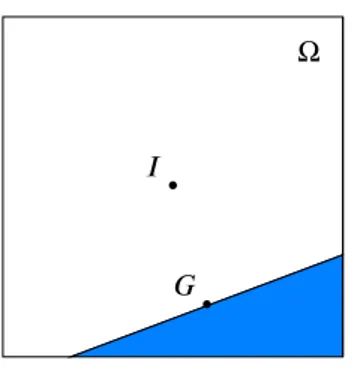
with 𝑃𝐺the pressure at wall (see Figure 1), 𝑃𝐼 the pressure at 𝐼 and ⃗𝐼 𝐺the vector between the corrected cell center of gravity and the solid face center of gravity.
Then, the pressure force acting on a solid is computed with:
⃗
𝐹𝑝𝑟𝑒𝑠𝑠𝑢𝑟𝑒 = ∫
Ω
𝑃𝐺𝑑𝑆⃗ (7)
As the assumption of the chosen two-fluid approach is to have a single pressure, the computation of the pressure force is unchanged in multi-phase flows.
∙
𝐼
∙
𝐺
Ω
FIGURE 1 Cell crossed by the fluid-structure interface, geometric characteristics re-shaping.
Friction contribution
For each cell having a porosity in]0, 1[, the friction contribution is computed at the wall. The velocity gradient is known in each cell. Consequently, the whole friction force is computed with:
⃗ 𝐹𝑓 𝑟𝑖𝑐𝑡𝑖𝑜𝑛 = ∫ Ω 𝜇(∇𝑈𝐺+ 𝑇 ∇𝑈𝐺) ⃗𝑑𝑆 (8)
In multi-phase flows, friction contribution from each phase 𝑘 is required. Therefore, for a cell 𝐼 :
⃗ 𝐹𝐼 , 𝑓 𝑟𝑖𝑐𝑡𝑖𝑜𝑛 = 𝑁 ∑ 𝑘=1 𝛼𝐼 ,𝑘 𝜀𝐼 𝜇𝑘(∇𝑈𝐼 𝑘 𝐺+ 𝑇 ∇𝑈 𝐼 𝑘 𝐺) ⃗𝑆𝐼 (9)
with N the number of phase. The sum of these contributions leads to the whole multi-phase friction force.
Gravity contribution
The mass of the structure is computed as:
𝑀𝑆 = 𝑁∑𝑐𝑒𝑙𝑙
𝐼=1
𝜌𝑠𝑜𝑙𝑖𝑑𝑉𝐼(1 − 𝜀𝐼) (10)
with 𝑁𝑐𝑒𝑙𝑙the number of cell in the domain, 𝜌𝑠𝑜𝑙𝑖𝑑the volumetric mass and 𝑉𝐼 the volume of the cell 𝐼 . Then, the gravity force applied on a structure S is written:
⃗
𝐹𝑔𝑟𝑎𝑣𝑖𝑡𝑦= 𝑀𝑆𝑔⃗ (11)
with ⃗𝑔the gravity.
Finally, the force acting on the structure is written:
⃗
𝐹𝑓 𝑙𝑢𝑖𝑑 = ⃗𝐹𝑝𝑟𝑒𝑠𝑠𝑢𝑟𝑒+ ⃗𝐹𝑓 𝑟𝑖𝑐𝑡𝑖𝑜𝑛+ ⃗𝐹𝑔𝑟𝑎𝑣𝑖𝑡𝑦 (12) Based on it, it is possible to predict the displacement of the structure.
3.2
Newmark algorithm
In order to compute the displacement of the structure due to the acting fluid forces, the following system is solved:
[𝑀]. ̈𝑋+ [𝐶]. ̇𝑋+ [𝐾].𝑋 = 𝐹 (13) with X a 3D displacement vector; M, C, K are the (3,3) mass, damping, and stiffness matrices. The resolution of this second order linear differential equation of the structure is carried out in space by the Newmark method17. In order to compute the
displacement and the velocity discretization, 𝛾 and 𝛽 are defined such as:
̇
𝑋𝑡+Δ𝑡= ̇𝑋𝑡+ Δ𝑡.[(1 − 𝛾). ̈𝑋𝑡+ 𝛾. ̈𝑋𝑡+Δ𝑡] (14)
𝑋𝑡+Δ𝑡= 𝑋𝑡+ Δ𝑡. ̇𝑋𝑡+
Δ𝑡2
This approach is frequently used in mechanic since it allows to choose the order of integration, to introduce or not numerical damping, and is accurate. It is unconditionally stable for:
𝛾 > 0.5
2𝛽 > 𝛾 (16)
A positive numerical damping is introduced for 𝛿 > 0.5 and a negative for 𝛿 < 0.5. The most frequently combination used is
𝛿 = 0.5, 𝛽 = 0.25 given that there is no numerical damping introduced It is unconditionally stable, and is a 2nd order scheme. This combination is used in the present work.
3.3
Iterative implicit algorithm
The computation of a force at the wall is sensitive since the solid is moving. In order to reduce this error, this force and the displacement are determined iteratively. Step by step the solid is moved until convergence. The iterative implicit fluid-structure coupling scheme used with the Time and Space Dependent Porosity method is presented here:
Based on the fluid flow properties of the previous iteration, the forces are computed and relaxed to stabilize the convergence. Then, thanks to the Newmark algorithm, the displacement and the velocity of the solid are calculated and the fluid domain is solved depending on the new position of the solid. First, based on the updated fluid domain, the fluid forces at the wall were computed and compared to the previous one. In order to limit the number of sub-iteration to 3 (most of the time), we use the two first iterations to get an approximation of a converged value with a fixed-point method. If it does not work, another sub-iteration is realized in order to find the fixed-point. Then, the force computed from the third sub-sub-iteration is compared to this value in order to check the stability of this solution. The fluid domain is then restarted to its state at the beginning of the present iteration. When the comparison of the forces is under a certain tolerance, the flow is updated and the next iteration starts. The determination of the convergence criterion is described in the first validation case. This fluide-structure coupling would have been possible without sub-iteration by using very small time steps. Instead, with the present iterative implicit algorithm it is possible to use regular time-steps.
4
NUMERICAL VALIDATION OF THE FLUID-STRUCTURE COUPLING
In order to evaluate the fluid-structure coupling with the Time and Space Dependent Porosity method, three test cases are chosen:
• cylinder removed from its equilibrium position in a still fluid,
• flow-induced vibration of a free cylinder with 𝑅𝑒= 100,
• free fall of a spherical solid on a free surface.
A sensitivity to the time step and to the number of cycles is performed on the first test case. Then, for the second case, a wide range of reduced velocity is computed in order to validate the correct prediction of the amplitude. Finally, based on two experiments, the two-phase character of the force is challenged.
4.1
Cylinder removed from its equilibrium position in a still fluid
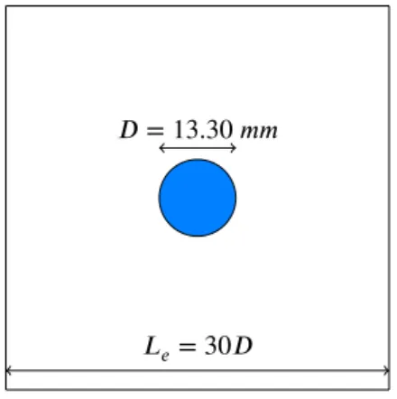
𝐿𝑒= 30𝐷
𝐷= 13.30 𝑚𝑚
FIGURE 2 Cylinder removed from its equilibrium position in a still fluid, geometry.
In order to get the added-mass and the damping coefficient in a fluid domain, a manner consists in removing a tube from its equilibrium position with a given amplitude and recording its response. Based on its response, added-mass and damping coefficient are deducted.
A cylinder with a diameter D is immersed in an incompressible fluid domain where the confinement coefficient is 𝐿𝑒∕𝐷 = 30 (with 𝐿𝑒the characteristic length of the domain). The fluid is water with a density 𝜌= 1000 𝑘𝑔∕𝑚3and a kinematic viscosity 𝜈= 10−6𝑚2∕𝑠. The tube is released without any velocity with an amplitude 𝑆
0= 0.001𝐷.
The tube is represented with a mass-spring system with damping:
̈ 𝑋𝑠+ 2𝜉𝑠𝜔𝑠𝑋̇𝑠+ 𝜔2𝑠𝑋𝑠= 0 (17) with 𝜔2 𝑠 = 𝐾𝑠∕𝑀𝑠and 𝜉𝑠= 𝐶𝑠 2𝜔𝑠𝑀𝑠
. The characteristics of the tube are 𝐷= 13.30 𝑚𝑚, 𝜔𝑠 = 99.90 𝑟𝑎𝑑∕𝑠, 𝜉𝑠 = 0.36%, and 𝑀𝑠= 0.298 𝑘𝑔∕𝑚.
When the tube is immersed in a fluid at rest, the fluid action is represented by an added mass 𝑀𝑎and a damping 𝐶𝑎:
𝑀𝑠( ̈𝑋𝑠+ 2𝜉𝑠𝜔𝑠𝑋̇𝑠+ 𝜔𝑠2𝑋𝑠) = −𝑀𝑎𝑋̈𝑠− 𝐶𝑎𝑋̇𝑠 (18)
Consequently,
(𝑀𝑠+ 𝑀𝑎) ̈𝑋𝑠+ (𝐶𝑎+ 𝐶𝑠) ̇𝑋𝑠+ 𝐾𝑠𝑋𝑠= 0 (19)
The objective is to numerically deduced the pulsation and the reduced damping of the system:
𝜔2𝑓 𝑠= 𝐾𝑠 (𝑀𝑠+ 𝑀𝑎)
and 𝜉𝑓 𝑠= 𝐶𝑠+ 𝐶𝑎 2𝜔𝑓 𝑠(𝑀𝑠+ 𝑀𝑎)
According to AMOVI experiment18, for low Reynolds number, the frequency of the system is 𝑓
𝑓 𝑠,𝑒𝑥𝑝= 12.866 𝐻𝑧 and reduced
damping 𝜉𝑓 𝑠,𝑒𝑥𝑝= 1.00%.
The geometry of the simulation is presented in Figure 2. The time step is constant and the maximum Courant number is under 1.
4.1.1
Sensitivity to the number of cycles
In the present study, a particular attention is paid to the tolerance in the fluid-structure coupling algorithm since it defines when the displacement is correctly predicted. Consequently, in order to determine it, we define 𝛿 like:
𝛿= (𝐹
𝑘+1− 𝐹𝑘
𝐹𝑘 )
2 (21)
with 𝐹𝑘+1and 𝐹𝑘forces computed respectively after 𝑘+ 1 and 𝑘 sub-cycles. The objective of this case is to show the importance
in the choice of a value for 𝛿𝑚𝑎𝑥to predict the displacement with a reasonable computational time.
Therefore, the displacement is computed with few constant numbers of sub-cycles from 2 to 15. Then, different runs are carried out with a fixed 𝛿𝑚𝑎𝑥from1.0 10−3to1.0 10−8.
FIGURE 3 Cylinder removed from its equilibrium position in a still fluid after 1 period on the left, after 31 periods on the right,
sub-cycles and 𝛿𝑚𝑎𝑥sensitivity.
In Figure 3, the displacement of the cylinder is presented after 1 and 31 periods of oscillation for different convergence criterion. According to the results, it appears that 2 and 5 sub-iterations are not enough. However, with 10 and 15 sub-cycles, the predictions of displacement are close. For 𝛿𝑚𝑎𝑥= 1.0 10−3, the criterion is distinctly not relevant to predict accurately the
displacement. In contrast,1.0 10−6and1.0 10−8are in agreement with the prediction of displacement with 10 and 15 sub-cycles.
1.0 10−5slightly under-estimates the displacement. This convergence might be time-consuming consequently a 𝛿
𝑚𝑎𝑥is chosen
in order to avoid unnecessary sub-cycles. Since we are working with strongly coupled problems, the choice for the following studies has been 𝛿𝑚𝑎𝑥= 1.0 10−6as a tolerance (between 2 and 10 sub-cycles are necessary at each iteration for the present case).
4.1.2
Sensitivity to the time step
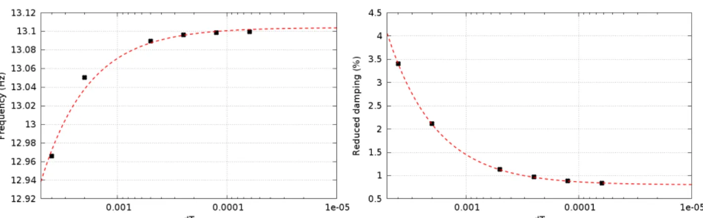
In Figure 4, a time step sensitivity is presented based on the intermediate refinement. The frequency and the reduced damping are computed for different time steps going from2.00 10−3to6.25 10−5𝑠. According to the results, the frequency is converging
FIGURE 4 Cylinder removed from its equilibrium position in a still fluid, time step sensitivity.
between them for frequency only. For damping, the error is probably due to the mesh refinement which is slightly too coarse to get the exact solutions.
Frequency (Hz) Reduced damping (%)
Experimental 12.866 1.000
Present Simulation, time step sensitivity 13.11 0.8
Error 1.89% 20%
Present Simulation, mesh sensitivity 13.07 1.01
Error 1.58% 1.0%
TABLE 1 Cylinder removed from its equilibrium position in a still fluid, numerical and experimental prediction of frequency
and reduced damping comparison.
4.1.3
Mesh sensitivity
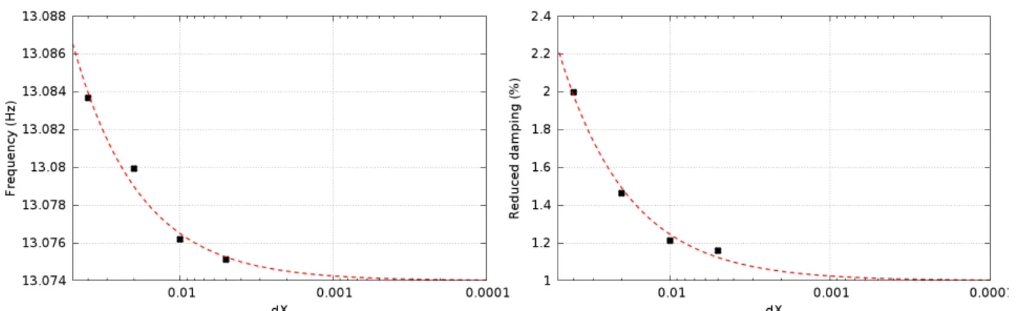
In Figure 5, a mesh sensitivity is presented for four meshes. Frequency and reduced damping are compared with experimental results in Table. 1 where it is possible to see how accurate is the numerical prediction. The present results show the correct choice of 𝛿.
Based on the present case, the tolerance required by the iterative algorithm is chosen equal to 𝛿𝑚𝑎𝑥= 1.0 10−6. A time and
space sensitivity studies are performed leading to accurate predictions of the displacement in terms of frequency and amplitude. Consequently, it is considered that the fluid-structure coupling algorithm is now ready to be used with the Time and Space Dependent Porosity method for application cases.
FIGURE 5 Cylinder removed from its equilibrium position in a still fluid, mesh sensitivity.
𝐿1= 8𝐷 𝐿2= 20𝐷
𝐻 = 20𝐷
𝐷
FIGURE 6 Flow-induced vibration of a free cylinder with 𝑅𝑒= 100, geometry.
4.2
Flow-induced vibration of a free cylinder with 𝑅𝑒
= 100
In the present case, we are interested in flow-induced vibration of a free-cylinder with 𝑅𝑒 = 100. In order to avoid boundary effects, the domain is considered infinite, that is why the size of the domain is large. In Figure 6, the domain used in the current work is presented. In order to insure a Reynolds number of 100, the flow characteristics are the diameter 𝐷= 0.025 𝑚, the inlet velocity 𝑈0= 4.0 10−3𝑚∕𝑠, the density 𝜌 = 1000 𝑘𝑔∕𝑚3and the dynamic viscosity 𝜇= 1.0 10−3𝑃 𝑎.𝑠.
Moreover, the prediction of the fluid force around the cylinder requires a fine mesh. The thickness of the smallest cells is 1.0 10−4𝑚around the cylinder. For this Reynolds number, it is allowed to work with a 2 dimensional domain (one cell in the third
direction). The left side is defined as the inlet, the right as the outlet. The cylinder wall is considered with a non-slip condition. Other surface are considered with a slip condition.
Fluid forces at wall are computed on the cylinder surface. Since the domain is 2 dimensional, they are divided by the length L of the cylinder which was chosen as 𝐿= 2.0 10−4𝑚. The drag and lift coefficient are then computed as:
𝐶𝑖= 𝐹𝑖 1 2𝜌𝑈 2 0𝐷𝐿 (22)
with 𝑖= 𝑥 or 𝑦. The fluid flow is unsteady and the maximum Courant number is taken under 1. In order to predict the correct vibration, the forces have to be correctly predicted. First, with a fixed cylinder, numerical results are compared to the result of19
in Table 2.
Numerical results are in correct agreement with19. The forces are consequently well predicted. The flow being fully developed,
𝐶𝑥,𝑎𝑣𝑒𝑟𝑎𝑔𝑒𝑑 𝐶𝑦,𝑚𝑎𝑥𝑖𝑚𝑢𝑚 Strouhal
19 1.389 0.328 0.166
Present Simulation 1.391 0.335 0.166
Error 0.1% 2.13% 0.005%
TABLE 2 Force coefficients and Strouhal prediction for a single-phase flow around a cylinder with 𝑅𝑒 = 100. Comparison between results from19and the present study.
First, we respectively define the reduced mass and the reduced stiffness:
𝑚∗ = 𝑚 1 2𝜌𝐷 2𝐿 = 𝜋 2 𝜌𝑠𝑜𝑙𝑖𝑑 𝜌 (23)
with 𝑚 the mass of the cylinder, and 𝜌𝑠𝑜𝑙𝑖𝑑the volumetric mass of the cylinder.
𝑘∗= 𝑘 1 2𝜌𝑈 2 0 (24)
The present cases are based on the work of20who explores a large range of reduced mass and stiffness with zero damping.
In Figure 7, an example of velocity field around the free-cylinder is proposed for 𝑚∗ = 1.25 and 𝑘∗ = 2.48. The amplitude of displacement is here 60% of the diameter. It is possible to see the vortex shedding by looking at the different snapshots.
FIGURE 7 Flow-induced vibration at 𝑅𝑒= 100 for 𝑚∗= 1.25 and 𝑘∗ = 2.48. Picture of the cylinder displacement and a vortex
In Table 3, we present the characteristics of the cases computed in the present study. Since the application of the thesis is a cross-flow in a tube-bundle where 𝑚∗ >1, we only consider cases with 𝑚∗ >1. Cases with 𝑚∗ <1 would be more difficult to
simulate and would require a different coupling method which is not of primary interest here.
Case A B C D E F G H I J
𝑚∗ 4.00 2.50 1.50 5.00 5.00 10.0 15.0 1.25 2.50 5.00
𝑘∗ 0.0 0.0 0.0 4.74 9.88 19.78 29.68 2.48 4.96 8.74
TABLE 3 Numerical cases from20computed in the present study.
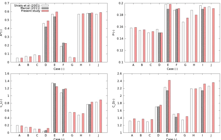
FIGURE 8 Response for undamped systems for various cases: 𝐴∗amplitude, 𝑓∗frequency, 𝐶
𝐿max lift coefficient and 𝐶𝐷,𝑎𝑣
averaged drag coefficient. Comparison between numerical results from20,21and the present method.
In Figure 8, numerical results from20,21and the present method are compared for a wide range of reduced-mass and damping.
Amplitude, frequency, maximum lift coefficient and time-averaged drag coefficients are presented in the four different graphics. The amplitude of vibration predicted by the present method is in a correct agreement with the others. The major discrep-ancy seems to be for case D and F where the characteristic shedding frequency is going to coincide with the natural structural frequency. The other parameters are also correctly predicted by the present method.
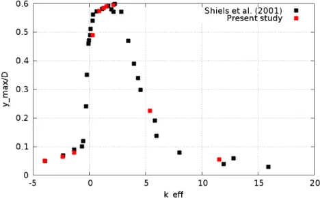
FIGURE 9 Response for undamped systems plotted against effective elasticity. Comparison between numerical results from20
and the present method.
In Figure 9, the response for undamped cases presented previously is plotted against effective elasticity (defined in20). It
appears that the maximum amplitude is the same with both methods. Moreover, the variation of amplitude with effective elasticity (which is dependent on 𝑘∗, 𝑚∗and 𝑓∗) are approximatively the same.
These results are very encouraging since the fluid-structure method based on an immersed approach leads to predictions in agreement with the ones based on ALE approach (Arbitrary Lagrangian Eulerian22). It is consequently a concrete validation in
single-phase flow of our method. In the following section, an application case is performed with two-phase flow.
For the present case, with a mesh of 100 000 cells, CPU time was about 2 hours on 100 cores tp compute a physical time of 1000s. Three FSI-sub-cycles were needed per iteration and the solid computation was about 5% of the CPU time per iteration.
4.3
Free fall of a spherical solid on a free surface.
The present case deals with free-fall of spheres from air to water performed experimentally by23. A sphere is held at height
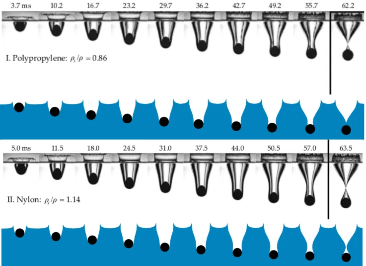
H above a water tank. The tank has dimensions of 30x50x60 𝑐𝑚3. The sphere is released from rest and falls toward the water, reaching it with approximate speed 𝑈0=√2𝑔𝐻0, with 𝐻0the initial altitude of the sphere. The geometry is presented in Figure 10. The impact sequence is recorded with high speed camera. The trajectory of the sphere and its impact speed are determined based on records. Spheres are made of different materials: polypropylene, nylon, teflon and steel. Their densities are respectively 0.86, 1.14, 2.30, and 7.86 𝑘𝑔∕𝑐𝑚3.
The impact of a sphere on water creates subsurface air cavity which are different depending on the material. As the sphere falls, it transfers momentum to the water by forcing it radially outward. This inertial expansion of the fluid is resisted by hydrostatic pressure which eventually reverses the direction of the radial flow, thereby initiating cavity collapse. The collapse accelerates until the moment of pinch-off, at which the cavity is divided into two separate cavities. The most obvious differences between the four impact sequences are the trajectories of the spheres. As the sphere density decreases, several trends are readily apparent:
• the depth of pinch-off decreases
• the depth of the sphere at pinch-off decreases
• the pinch off depth approaches the sphere depth at pinch-off.
The diameter of the sphere is 𝐷= 2.54 𝑐𝑚, the impact velocity is 𝑈𝑧 = −217 𝑐𝑚∕𝑠. The air and water are at rest at the initial
state. The air influence from the fall before impact is consequently neglected.
In order to simulate the phenomenon, a 3D-mesh is used since it is a sphere. The dimension of the tank are respected to avoid pressure field discrepancies. The free surface is computed thanks to the Large Interface Model presented in appendix. There is no turbulence model. The time step is adaptive and the maximum Courant number remains under 1.
𝐻𝑤𝑎𝑡𝑒𝑟= 60 𝑐𝑚 𝐷= 2.54 𝑐𝑚
𝑈𝑧= −217 𝑐𝑚∕𝑠
Water at rest
Air at rest
FIGURE 10 Confined cylinder released in a fluid, geometry.
First, a mesh refinement study is performed. The chosen material is the teflon. The simulation is performed on 3 refinements of 100 000, 500 000 and 2 500 000 cells. These different meshes are refined along the sphere trajectories. In Figure 11, trajectories of a teflon sphere are plotted along time for the 3 refinements. The coarse mesh seems to slightly underestimate the depth along time. However, mesh 2 and 3 are in correct agreement along time with the experimental data.
FIGURE 11 Free-fall of a sphere on a free-surface: mesh refinement for teflon (on the left). Numerical/experimental
displacement along time of a sphere free-falling on a free surface for 4 different materials (on the right).
According to the previous result, the numerical simulation are performed with the mesh 3. With three other materials (polypropylene, nylon and steel), the same test case is computed. In Figure 11, numerical and experimental trajectories are com-pared. There is a correct agreement between them. Consequently, the effort of the water entry coming from water and air are correctly reproduced with our numerical model.
Based on the snapshots of the free-fall (see Figure 12 and 13), it is possible to find the pinch-off time. Another method is to use the velocity where a radical change happens exactly at the pinch-off. Since the experimental pinch-off time are available, a confrontation with numerical results is performed in Table.4. There is an excellent agreement between simulation and experiment for the pinch-off time prediction. Moreover, Figure 11 highlights the correct prediction of the pinch-off depth and time since there is a maximum of 5% of error.
Polypropylene Nylon Teflon Steel Experiment (𝑠) 62.2 63.5 66.1 68.9 Simulation (𝑠) 61.5 63.1 65.8 68.7 Error (−) 1.11% 0.62% 0.46% 0.2%
TABLE 4 Numerical and experimental pinch-off time comparison.
In Figure 12 and 13 based on the snapshots given in the experimental study, the numerical simulations are compared along time. For the different materials, the air-water interface is correctly reproduced by the simulation. This case is consequently the first two-phase flow application using the Time and Space Dependent Porosity method with a fluid-structure coupling.
FIGURE 12 Polypropylene and nylon spheres falling on a free surface of water. Numerical (bottom) and experimental (top)
snapshot of the sphere entry in water.
For the present case, with a mesh of 2 500 000 cells, CPU time was about 2 hours on 224 cores. Three FSI-sub-cycles were needed per iteration and the solid computation was about 5% of the CPU time per iteration.
FIGURE 13 Teflon and steel spheres falling on a free surface of water. Numerical (bottom) and experimental (top) snapshot of
the sphere entry in water.
SUMMARY AND REMARKS
After a short description of existing fluid-structure coupling algorithm, the present algorithm has been presented. The computa-tion of the force at wall with the Time and Space Dependent Porosity method is highlighted since it is not convencomputa-tional. In order to predict the displacement of the structure, a Newmark algorithm is used. Finally, the iterative implicit fluid-structure coupling is described.
Based on three different cases, the coupling is validated before going through the targeted application. First, with the cylinder removed from its equilibrium position in a still fluid, the tolerance parameter to stop iterations is determined. Then, flow-induced vibrations of a cylinder at 𝑅𝑒= 100 are predicted for different values of mass and stiffness. This has been the first case of flow-induced vibration using the Time and Space Dependent Porosity method with its fluid-structure interaction module. Finally,
a fluid-structure interaction case in two-phase flow is realized. Here, the free-fall of a sphere on a free-surface is studied and compared with experimental results.
Because of the computational time, we did not perform the free-fall of sphere on a liquid-liquid free-surface with high vis-cosities and densities from24,25. A perspective is to perform these case since the two-phase character of the force is highly
challenged. These cases are of primary interest since they validate fluid-structure interaction with two-phase flow.
The use of an immersed boundary method to perform fluid-structure interaction is comfortable since it allows large or slight displacement without any dependency on the mesh and consequently to work on complex industrial applications such as hydraulic dashpots for example. In hydraulic dashpots, the free-falling structures slow down because of the reduced distance between the structure and the wall. Therefore, there is large displacement with a very slight thickness between the structure and the wall. The prediction of the structure displacement in this configuration is possible with the FSI module developed in the present work.
A perspective of development is to implement the coupling for rotation since only translation is considered for now. Applications like wind turbines or water wheels would be possible to study with the present method.
It is now possible to predict the motion of structure induced by a two-phase flow. A concrete development and validation step has been carried out. Consequently, all the technical tools are gathered to simulate two-phase flows induce vibration in steam generator tube bundle for example.
ACKNOWLEDGMENT
Authors want to thank both EDF R&D projects: Qual-IFS-GV, devoted to the assessment of SG tube vibration risk; and NEPTUNE funded by EDF (Electricité de France), CEA (Commissariat à l’Energie Atomique et aux Energies Alternatives), Framatome and IRSN (Institut de Radioprotection et de Sureté Nucléaire).
References
1. Benguigui W, Doradoux A, Lavieville J, Mimouni S, Longatte E. A discrete forcing method dedicated to moving bodies in two-phase flows. International Journal of Numerical Methods in Fluids 2018.
2. Étienne S, Pelletier D. A general approach to sensitivity analysis of fluid–structure interactions. Journal of Fluids and
Structures2005; 21(2): 169 - 186. doi: https://doi.org/10.1016/j.jfluidstructs.2005.07.001
3. Hübner B, Walhorn E, Dinkler D. A monolithic approach to fluid–structure interaction using space–time finite elements. Computer Methods in Applied Mechanics and Engineering 2004; 193(23): 2087 - 2104. doi: https://doi.org/10.1016/j.cma.2004.01.024
4. Matthies HG, Steindorf J. Partitioned but strongly coupled iteration schemes for nonlinear fluid–structure interaction.
Computers & Structures2002; 80(27): 1991 - 1999. doi: https://doi.org/10.1016/S0045-7949(02)00259-6
5. Matthies HG, Steindorf J. Partitioned strong coupling algorithms for fluid–structure interaction. Computers & Structures 2003; 81(8): 805 - 812. K.J Bathe 60th Anniversary Issuedoi: https://doi.org/10.1016/S0045-7949(02)00409-1
6. Huvelin F, Longatte E, Verreman V, Soulie Y. Numerical Simulation of Dynamic Instability for a Pipe Conveying Fluid.
Pressure Vessel and Piping2006.
7. Matthies HG, Niekamp R, Steindorf J. Algorithms for strong coupling procedures. Computer Methods in Applied Mechanics
and Engineering2006; 195(17): 2028 - 2049. Fluid-Structure Interactiondoi: https://doi.org/10.1016/j.cma.2004.11.032
8. Hou G, Wang J, Layton A. Numerical Methods for Fluid-Structure Interaction — A Review. Communications in
Computational Physics2012; 12(2): 337–377.
9. Küttler U, Wall W. Fixed-point fluid-structure interaction solvers with dynamic relaxation. Computational Mechanics 2008; 43: 61-72.
10. Song M, Lefrançois E, Rachik M. A partitioned coupling scheme extended to structures interacting with high-density fluid flows. Journal of Computers & Fluids 2013; 84: 190–202.
11. Guelfi A, Bestion D, Boucker M, et al. A. Guelfi, D. Bestion, M. Boucker, P. Boudier, P. Fillion, M. Grandotto, J.-M. Hérard, E. Hervieu, P.Peturaud.. Nuclear Science and Engineering 2007.
12. Ishii M. Thermo-fluid dynamic, theory of two-phase. Eyrolles . 1975.
13. Mimouni S, Archambeau F, Boucker M, Lavieville J, Morel C. A second order turbulence model based on a Reynolds stress approach for two-phase boiling flow and application to fuel assembly analysis. Nuclear Engineering and Design 2010.
14. Coste P. A Large Interface Model for two-phase CFD. Nuclear Engineering and Design 2013; 255: 38-50.
15. Merigoux N, Lavieville J, Mimouni S, Guingo M, Baudry C. A generalized large interface to dispersed bubbly flow approach to model two-phase flows in nuclear power plant. CFD4NRS-6, Boston 2016.
16. Denèfle R, Mimouni S, Caltagirone J, Vincent S. Multifield hybrid approach for two-phase flow modeling - Part 1: Adiabatic flows. Journal of Computers & Fluids 2014.
17. Newmark N. A method of computation for structural dynamics. Journal of Engineering Mechanics 1959: 67-94.
18. Baj F. Amortissement et instabilité fluide-elastique d’un faisceau de tubes sous écoulement diphasique. Thèse de doctorat,
Université Paris VI1998.
19. Pomarede M, Longatte E, Sigrist J. Numerical simulation of an elementary vortex-induced-vibration problem by using a fully coupled fluid solid system computation. International Journal of Multiphysics 2010; 4(3): 273-291.
20. Shiels D, Leonard A, Roshko A. Flow-induced vibration of a circular cylinder at limiting structural parameters. Journal of
Fluids and Structures2001; 15: 3-21.
21. Marcel T. Simulation numérique et modélisation de la turbulence statistique et hybride dans un écoulement de faisceau de tubes à nombre de Reynolds élevé dans le contexte de l’interaction fluide-structure. Thèse de doctorat, Université de
Toulouse2010.
22. Noh . A time dependant two-space-dimensional coupled eulerian-lagrangian code. W.F.alderb edn. Academic Press 1964.
23. Aristoff J, Truscott T, Bush ATJ. The water entry of decelerating spheres. Physics of fluids 2010; 22.
24. Pierson J, Magnaudet J. Inertial settling of a sphere through an interface. Part 1. From sphere flotation to wake fragmentation.
Journal of Fluid Mechanics2018; 835: 762-807.
25. Pierson J, Magnaudet J. Inertial settling of a sphere through an interface. Part 2. Sphere and tail dynamics. Journal of Fluid