HAL Id: hal-02321581
https://hal.inria.fr/hal-02321581
Submitted on 21 Oct 2019
HAL is a multi-disciplinary open access
archive for the deposit and dissemination of
sci-entific research documents, whether they are
pub-lished or not. The documents may come from
L’archive ouverte pluridisciplinaire HAL, est
destinée au dépôt et à la diffusion de documents
scientifiques de niveau recherche, publiés ou non,
émanant des établissements d’enseignement et de
A Comparative Study of Neural Network Compression
Hossein Baktash, Emanuele Natale, Laurent Viennot
To cite this version:
Hossein Baktash, Emanuele Natale, Laurent Viennot. A Comparative Study of Neural Network
Com-pression. [Research Report] INRIA Sophia Antipolis - I3S. 2019. �hal-02321581�
A Comparative Study of Neural Network
Compression
Hossein Baktash
∗Sharif University of Technology, Iran
Emanuele Natale
CNRS, UCA, I3S, INRIA, France
Laurent Viennot
INRIA, IRIF, France
October 21, 2019
Abstract
There has recently been an increasing desire to evaluate neural net-works locally on computationally-limited devices in order to exploit their recent effectiveness for several applications; such effectiveness has nev-ertheless come together with a considerable increase in the size of mod-ern neural networks, which constitute a major downside in several of the aforementioned computationally-limited settings. There has thus been a demand of compression techniques for neural networks. Several proposal in this direction have been made, which famously include hashing-based methods and pruning-based ones. However, the evaluation of the efficacy of these techniques has so far been heterogeneous, with no clear evidence in favor of any of them over the others.
The goal of this work is to address this latter issue by providing a comparative study. While most previous studies test the capability of a technique in reducing the number of parameters of state-of-the-art net-works, we follow [CWT+15] in evaluating their performance on basic ar-chitectures on the MNIST dataset and variants of it, which allows for a clearer analysis of some aspects of their behavior. To the best of our knowledge, we are the first to directly compare famous approaches such as HashedNet, Optimal Brain Damage (OBD), and magnitude-based prun-ing with L1 and L2 regularization among them and against equivalent-size feed-forward neural networks with simple (fully-connected) and structural (convolutional) neural networks. Rather surprisingly, our experiments show that (iterative) pruning-based methods are substantially better than the HashedNet architecture, whose compression doesn’t appear advanta-geous to a carefully chosen convolutional network. We also show that, when the compression level is high, the famous OBD pruning heuristics deteriorates to the point of being less efficient than simple magnitude-based techniques.
∗Contributed to the paper during a summer internship in INRIA Sophia Antipolis, France,
1
Introduction
Because of their increasing use in applications over mobile devices and em-bedded systems, there has been recent surge of interest in developing methods to reduce the size of neural networks [HWC18]. The Moving Picture Experts Group, for example, recently opened a part of the MPEG-7 Standard in order to standardize aspects of neural networks compression for multimedia content description and analysis [Gro19]. In the primary setting which is considered in this context, the client on which the networks has to be stored and evaluated has weak storage and computational capabilities, while the server on which the network is trained can be assumed to be a high-performance cluster.
The neural-network compression techniques explored so far can be sum-marily grouped in the following main families of strategies: matrix decom-position methods, such as low-rank decomdecom-positions [LWF+15]; weight-sharing techniques, such as hashing-based and quantization schemes [HWC18]; pruning techniques, such as Optimal Brain Damage (OBD) [LCDS89] and other iterative pruning-based methods.
The motivation for this work stems from what appears to be a major gap in the literature encompassing these techniques, as for a satisfying and methodical assessment of their relative efficacy. In fact, the series of works exploring these methods has been quite heterogeneous with respect to the way they have been compared to each other. We thus aim for a principled comparison which provides substantial evidence in favor of some of them over the others. The main principle at the basis of our study is to strive for the most minimalist setting: we consider simple architectures with a single hidden layer and perform our experiments on the classical MNIST dataset and variants of it [LEC+07], in opposition to
most previous work which focused on reducing the number of parameters of state-of-the-art architectures. Such choices allow for a clearer analysis of some aspects of the behavior of the technique. A similar approach has been adopted in [CWT+15] (with some limitations that we discuss in the Related Work section). We now briefly discuss the compression methods we consider. Further de-tails are provided in the Related Work and technical section of the paper. We first remark that, while low-rank methods have been shown to achieve good speed-ups for large convolutional kernels, they usually perform poorly for small kernels [HWC18], and appear inferior to hashing-based methods [CWT+15]. We
thus focus on the two other classes of techniques. Hashing-based schemes, in particular, have attracted much attention. The central idea behind them is to employ hash functions to randomly group edges in buckets, and then constrain edges belonging to the same bucket to share the same weight. In this work, we focus on the main representative of this family of methods, namely the Hashed-Net architecture [CWT+15] . The third family of techniques, (iterative) pruning
methods, date back to the seminal work by LeCun et al. in 1989 on the Optimal Brain Damage (OBD) technique [LCDS89], and have recently regained attention [ZG18, ZJN18]. For brevity’s sake, we omit the adjective iterative in the rest of the paper, since we don’t consider non-iterative pruning methods. In pruning methods, the central idea is to sparsify the network during training by choosing
some edges to be removed. While in OBD and older methods the choice of edges to be removed is made according to heuristics that aims at minimizing the loss of the network accuracy, recent work has focused on magnitude-based methods, in which the edges to be removed are simply those with the smallest absolute value. Rather surprisingly, recent work do not validate their results against the aforementioned older methods.
1.0.1 Our Contribution
To the best of our knowledge, this is the first work that provide an explicit com-parison of compression approaches such as HashedNet, OBD and magnitude-based pruning with L1 and L2 regularization, which we also compare against convolutional networks with number of parameters equivalent to that of the the final compressed network (see the Discussion section where we argue that convolutional networks can be regarded as a structured weigh-sharing method). Rather surprisingly, our experiments show that pruning methods are substan-tially better than the HashedNet architecture, whose compression doesn’t ap-pear advantageous to a carefully chosen convolutional network. Even more interestingly, magnitude-based pruning appear to perform at least as good as OBD, outperforming it consistently when the compression ratio1 lead to very
sparse topologies. It has been already noted in the literature that the assump-tions on which the OBD heuristic is based on fail to hold in practice [HSW93]: our results show that this is true to the extent that magnitude-based edge-removal turns out to be a better heuristic for minimizing the accuracy loss. The reader will find a discussion on the above results and further consequences of our experiments in the Discussion section. Overall, while surely not exhaustive, our work assess the relative efficacy of neural-network compression methods in a basic setting, and it provides fundamental insights on their shortcomings and strengths.
2
Related Work
In this section we provide an overview on the works that concern the main neural-network compression techniques. Before discussing the individual fami-lies of methods, we observe that the general justification for the search of efficient neural-network compression methods lies in the empirical observation that for natural tasks most network parameters appear to be redundant, as they can be accurately predicted from a small fraction of them [DSD+13]. We also note
that a famous approach to reduce the number of network parameters which we don’t consider in this work is that of Dark Knowledge [HVD15]. We ex-clude such technique based on the fact that [CWT+15] shows that the method
doesn’t match the performance of their HashedNet; moreover, while [CWT+15]
1The compression ratio is defined as r :=m0
m where m is the number of parameters of the
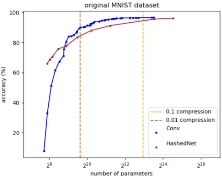
Figure 1: Accuracies of the HashedNet and convolutional network architec-tures, based on the number of parameters, on the MNIST dataset. The results for HashedNet are obtained by compressing a network with 100 hidden units in a single hidden layer from 0% compression up to 99% compression. The convolutional networks consistently outperform HashedNet.
combines HashedNet with Dark Knowledge, as we discussed in the Experiment section, in this work we avoid combining different methods.
2.1
Hashing-based Techniques
Hashing-based techniques for neural network compression have been introduced in [CWT+15], which proposed the HashedNet architecture. The idea of the
tech-nique is to randomly hash the network edges into buckets and then constrain all edges between the same bucket into having the same weight. They can thus be naturally interpreted as weight-sharing schemes, and regarded as dimensionality reduction steps between network layers such as feature hashing [CWT+15] and
random linear sketching [LSY19]. We remark that, in [CWT+15] and in later
works, HashedNet has not been directly compared to iterative pruning tech-niques. Recently, [LSY19] provided rigorous theoretical results on the convexity of the optimization landscape of one-hidden-layer HashedNet, showing that it is similar to that of a simple (one-hidden-layer) fully-connected network.
Figure 2: Accuracies of pruning methods and simple convolutional networks, with almost the same number of parameters on the MNIST dataset. The results for the pruning methods are obtained by compressing fully connected networks with 100 hidden units, starting from 0% compression up to 99% compression.
[CWT+16] have successively applied the HashedNet technique to the
fre-quency domain, by first converting filter weights to the frefre-quency domain with a discrete cosine transform before applying the HashedNet technique.
While HashedNet and many of its variants initially group edges in different buckets before training, in unrestricted-server settings, [HWC18] shows that an improved hashing scheme can be computed, in order to obtain the best approx-imation of an uncompressed network trained for the given task. In particular, [HWC18] adapts previous results for computing inner-product-preserving hash-ing functions in order to obtain a good binary-weight approximation of the given neural network.
2.2
Pruning-based Techniques
An iterative pruning methods is generally identified by its measure of edge saliency, i.e. a way to associate a value to individual edges so that edges with the lowest value should be pruned first, and its pruning schedule, that is way to decide when the pruning should happen and how many edges should be pruned
Figure 3: Accuracies of pruning methods and simple convolutional networks with almost the same number of parameters on the rotated MNIST dataset. The results are obtained by compressing fully connected networks with 100 hidden units, starting from 0% compression up to 99% compression.
[ZG18].
2.2.1 Optimal Brain Damage
The earliest, famous example of pruning method is Optimal Brain Damage (OBD) [LCDS89]. Starting from the consideration that the pruning operation should attempt to increase the value of the loss function by the least possible amount, OBD proposes the following heuristic to determine edge saliencies: the loss function is first approximated via its Taylor expansion up to the second order, thus leading to a formula which include its gradient and its Hessian; first, in order to be able to ignore the linear factor involving the gradient, OBD sets the pruning to take place when the training appears to have reached a local minimum; then, since the Hessian would be unfeasible to estimate, it crucially assumes that the extra-diagonal entries of the Hessian matrix can be assumed to be zero. for a formal presentation of the above procedure, we defer the reader to the original paper [LCDS89] . Thanks to the above assumption, OBD is able to compute saliency efficiently. In the original paper [LCDS89], it is shown that OBD leads to a much better accuracy than a simpler magnitude-based method.
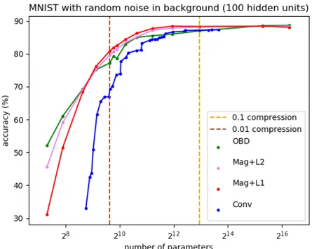
Figure 4: Accuracies of pruning methods and simple convolutional network with almost the same number of parameters on the MNIST dataset with random background. The results are obtained by compressing fully connected networks with 100 hidden units, starting from 0% compression up to 99% compression.
Successively, [HSW93] and [HSW94] proposed Optimal Brain Surgeon (OBS). They argue that OBD’s assumption of zero extra-diagonal entries for the Hes-sian fails to be satisfied in typical tasks, and they base their OBS on an exact expression for the saliency drop due to an edge deletion; however, their method reintroduce a quadratic time complexity for estimating the Hessian, and is thus unfeasible for non-small networks.
2.2.2 Magnitude-based Pruning
Magnitude-based pruning methods simply define the saliency of an edge to be its absolute value, and have recently gained popularity as a simple yet effec-tive neural-network compression method [ZG18, ARMK18], also thanks to its versatility in combining with other methods [HMD15, HPTD15]. In particular, [ZG18] consider a magnitude-based pruning method2 that at the ith step of pruning reaches a sparsity level of r(1 − (1 −ki)3), where r is the desired
com-2We have been unable to determine whether the magnitude-based pruning considered in
Figure 5: Accuracies of pruning methods and simple convolutional network with almost the same number of parameters on the MNIST dataset with images in background. The results are obtained by compressing fully connected networks with 100 hidden units, starting from 0% compression up to 99% compression.
pression ratio and k is the total number of pruning steps, which is a pruning schedule which bears some similarity to those adopted in our pruning methods. We remark again that, although recent works investigating magnitude-based pruning techniques mention OBD as a related method, they fail to test the latter against their method.
3
Description of Compression Methods
In this section we describe in details the neural network compression methods that we experimented with.
3.1
Description of HashedNet
Our experiments include the HashedNet architecture, introduced by [CWT+15].
pro-MagL2 100 hidden units one hidden layer edges removed mnist mnist background images mnist background random mnist rotation 0 % 97.650.11 82.040.13 88.440.23 89.160.56 50 % 97.690.05 82.430.12 88.330.38 88.720.45 90 % 96.990.18 81.870.54 88.150.64 86.750.37 95 % 96.620.23 81.800.41 87.840.47 85.410.58 97 % 96.020.25 80.920.52 87.160.41 82.750.38 98 % 95.520.13 79.920.55 85.100.18 79.000.48 98.5 % 94.940.19 78.710.66 83.400.23 75.550.21 98.8 % 94.500.18 77.620.36 81.380.32 72.000.50 98.9 % 94.540.16 76.890.44 80.560.39 70.510.41 99 % 94.310.17 75.980.45 79.570.34 68.761.09 99.3 % 93.000.22 72.161.04 75.140.24 62.171.55 99.5 % 91.090.20 68.170.41 69.150.66 53.970.39 99.7 % 84.691.01 58.453.05 59.112.19 41.802.65 99.8 % 74.252.14 47.302.30 45.541.79 32.981.86
Table 1: Results obtained by compressing a fully connected network with 100 hidden units with magnitude-based pruning with L2 regularization. The stan-dard deviation of the accuracies over independent runs (5 runs each) is given as a subscript to each entry.
vided by the authors3. The results of our experiments are shown in 1. As we discuss in Discussion of Convolutional Networks, carefully chosen convolutional architectures turn out to outperform this method across all compression ratios.
In the HashedNet architecture with m edges and compression ratio m k, the
network is initialized by assigning, for each layer, each edge to one out of k buckets, and by constraining the edges assigned to the same bucket to always have the same weight. The assignment is implemented using a hash function f ((i, j)), where edge (i, j) refers to the edge connecting nodes i and j in next and previous layers. In order to evaluate HashedNet, the weight of each edge (i, j) is retrieved by looking up the weight associated to its corresponding bucket f ((i, j)). As for training the HashedNet architecture, as it turns out by the back-propagation algorithm, the gradient of a bucket can be computed by summing up the gradients that all the edges assigned to the given bucket would have had, if they were allowed to have distinct weights.
3.2
Description of Pruning Methods
In (iterative) pruning methods, the desired compression level is achieved in multiple pruning steps. Each pruning step is performed every given number of
3The code can be found at http://web.archive.org/web/20190902141837/https://www.
MagL1 30 hidden units one hidden layer edges removed mnist mnist background images mnist background random mnist rotation 90 % 95.870.18 78.300.59 85.970.19 80.620.59 95 % 95.150.15 77.720.23 83.960.12 75.990.85 97 % 94.380.06 76.400.29 80.640.62 70.850.87 98 % 93.280.11 73.540.62 76.780.61 65.200.67 98.5 % 91.710.12 70.890.54 72.510.91 58.342.05 98.8 % 90.040.53 68.030.53 69.091.14 54.380.65 98.9 % 89.721.13 67.020.47 67.921.35 51.141.15 99 % 88.260.91 65.740.34 65.461.42 49.200.68
Table 2: Results obtained by compressing a fully connected network with 30 hidden units with magnitude-based pruning with L1 regularization. The stan-dard deviation of the accuracies over independent runs (5 runs each) is given as a subscript to each entry.
retraining epochs from the last pruning step, after which edges with the least saliency are removed. The adopted measure of saliency of an edge depends on the pruning method under consideration.
More specifically in OBD [LCDS89], the saliency of an edge with weight w is defined to be w2 ∂∂w2L2 (see the Related Work section for further details on such
rule). In magnitude-based pruning methods (here, Mag-L1 and Mag-L2), the saliency of an edge w is simply |w|.
After terminating the pruning steps by reaching the desired sparsity level, the network is trained for additional epochs until the accuracy reaches a local maximum.
3.2.1 Insights on the Pruning Schedule
Compared to pruning big chunks of edges at once, the purpose of reaching the desired compression by progressively pruning edges in multiple steps is to avoid sudden and unrecoverable accuracy drops [LCDS89, ZG18]. However, while pruning very few edges at every step would help in reducing the deterioration of the network accuracy, it would require an excessive increase in the number of epochs. On the one hand, bigger chunks of weights could be safely pruned as long as the network is above a certain level of edge density; on the other hand, sparse networks turns out to be more sensitive to the removal of edges, which suggests that pruning should be performed more gradually when the edge density becomes low. We thus employ iterative pruning methods which prune many edges in early phases of the training process and less edges in later ones, and which continue training the network for a certain number of epochs before and after each pruning phase.
MagL1 100 hidden units one hidden layer edges removed mnist mnist background images mnist background random mnist rotation 0 % 96.770.11 80.720.64 88.070.61 84.560.29 50 % 96.770.02 81.480.61 88.420.24 84.900.85 90 % 96.430.15 81.880.43 88.290.37 85.150.95 95 % 96.320.16 81.380.28 88.420.21 84.050.76 97 % 96.090.13 81.060.27 87.710.41 82.400.45 98 % 95.700.26 80.770.52 86.240.32 79.270.75 98.5 % 95.320.09 79.760.40 84.340.28 76.810.76 98.8 % 94.920.18 78.580.58 82.500.37 73.510.64 98.9 % 94.610.19 78.160.30 81.840.62 72.130.45 99 % 94.310.20 77.850.24 80.830.29 70.441.05 99.3 % 93.460.32 73.360.59 76.120.54 62.541.14 99.5 % 91.390.12 68.970.76 68.392.64 53.451.18 99.7 % 84.370.94 56.211.23 51.471.04 37.630.92 99.8 % 65.594.61 44.034.41 31.084.09 21.785.52
Table 3: Results obtained by compressing a fully connected network with 100 hidden units with magnitude-based pruning with L1 regularization. The stan-dard deviation of the accuracies over independent runs (5 runs each) is given as a subscript to each entry.
c
q
i
kS, where S is the final desired sparsity, k is the total number of pruning
steps and c ≥ 1 is a constant. As a consequence, in the later pruning steps, less edges are removed (the exact amount is controlled by c), and we have less dramatic accuracy drops (this is controlled by k). In the Related Work section, we mention a similar method for iterative pruning that has been used in [ZG18]. We remark that, in our experiments, we choose our parameter c such that, after the very few initial iterations, a much higher level of sparsity is reached compared to [ZG18]. The latter choice is motivated by the observation that, after the initialization of the weights according to a normal distribution with zero mean, the weight distribution has the tendency to remain normal with the same mean, with a strong concentration around zero; moreover, after several pruning steps, the weights tend to be less concentrated around zero, as can be seen in the histograms in Figure 6.
4
Experiments
Experiments are carried out on the MNIST dataset and some of its variants with 50000 training images and 12000 test images4. We varied the compression
4Note that in [LEC+07] they actually employed the set of 12000 images as training set
MagL2 30 hidden units one hidden layer edges removed mnist mnist background images mnist background random mnist rotation 90 % 95.770.08 75.520.74 82.690.23 78.990.30 95 % 94.980.08 75.030.36 81.311.16 75.700.49 97 % 94.270.26 74.120.53 79.250.49 71.210.58 98 % 93.200.11 72.840.29 76.520.55 65.970.74 98.5 % 91.610.48 70.230.68 73.770.16 59.560.90 98.8 % 90.100.21 68.880.37 70.730.77 56.520.96 98.9 % 89.580.08 67.341.11 70.190.52 53.341.03 99 % 87.890.53 66.160.47 68.060.59 51.700.48
Table 4: Results obtained by compressing a fully connected network with 30 hidden units with magnitude-based pruning with L2 regularization.The stan-dard deviation of the accuracies over independent runs (5 runs each) is given as a subscript to each entry.
ratios in the range [0.002, 0.1], and we tested simple architectures consisting of 100 and 30 hidden neurons within a single hidden layer. Of course for networks with 30 neurons we did not pursue a compression of less than 0.01, as it produced networks with very few parameters and very low accuracies that we did not find worth considering. Each set of parameters has been tested over 5 independent runs, in order to reduce the variability due to the random initialization of the weights and to the stochastic gradient descent algorithm5.
The average accuracies with their standard deviation can be seen in the tables from 1 to 6. To save space, we don’t include the rows corresponding to experiments with 30 hidden units and very low or very high compression, as the accuracy in those cases is very low and thus poorly informative.
In all experiments the magnitude-based pruning methods outperform the OBD and Convolution networks are beaten by all pruning methods with the same number of parameters (2). Also, among the other methods, the magnitude-based pruning with L1 regularization seems to outperform all others; this could be the result of the sparsification effect produced by the L1 regularization [GBC16, Section 7.1.2].
4.1
Experiments on Simple Convolutional Networks
We compare compressing methods to a simple convolution network with three hidden layers: a 2D convolution layer followed by a max pooling layer and a final linear layer. We try various values for the kernel size (from 5x5 to 10x10), the number of output channels (from 4 to 12), the stride (from 1 to 3) and the
relative size [Guy97], without justifying this choice; hence, here we switched the use of the two sets.
OBD 100 hidden units one hidden layer edges removed mnist mnist background images mnist background random mnist rotation 0 % 97.710.05 82.290.56 88.650.19 88.390.11 50 % 97.750.09 82.170.89 88.540.27 88.720.35 90 % 96.850.22 80.790.43 86.991.50 86.880.88 95 % 96.220.20 79.851.89 86.001.24 84.720.26 97 % 95.430.24 80.800.10 85.521.79 81.950.46 98 % 95.030.13 78.950.19 85.010.01 77.950.20 98.5 % 94.550.22 78.300.53 82.950.34 74.090.57 98.8 % 94.170.15 77.040.21 78.621.62 70.610.44 98.9 % 93.780.16 76.170.71 79.232.45 69.191.06 99 % 93.470.17 75.920.13 77.191.88 67.490.88 99.3 % 91.030.78 72.320.57 75.161.74 59.091.17 99.5 % 87.381.42 68.410.64 69.282.67 52.442.38 99.7 % 78.591.57 61.180.55 61.061.93 41.171.43 99.8 % 64.715.44 53.951.08 52.032.32 33.771.98
Table 5: Results obtained by compressing a fully connected network with 100 hidden units with the Optimal Brain Damage method. The standard deviation of the accuracies over independent runs (5 runs each) is given as a subscript to each entry.
pool size (from 2 to 4). We use a batch size of 16, a learning rate of 1e-2 and a L2 regularization with weight decay of 1e-3. We also try dropout between the max pooling layer and the linear layer (with probability from 0 to 0.2). The input is also normalized according to the mean and standard deviation of input values in the training set. For each set of parameters, we make 5 runs of training with 30 epochs and compute the average test accuracy at that point as well as the number of weights in the network. Among all our experiments, we show only those which are not Pareto dominated with respect to these two parameters (we ignore a set of parameters if another set of parameters provides better test accuracy with less weights).
We next give a rough description of the parameters yielding the best trade-offs of test accuracy versus number of weights. For highest accuracy, a larger number of output channels is used, and for most of the datasets, larger convo-lution size also. For reducing the number of weights, it seems better to increase the pool size. And only for very scarce number of weights, it becomes interesting to increase the stride. Larger dropout is used in the high accuracy regime while dropout does not seem beneficial in the low accuracy regime.
OBD 30 hidden units one hidden layer edges removed mnist mnist background images mnist background random mnist rotation 90 % 95.480.08 76.120.81 82.280.54 78.550.86 95 % 94.690.08 74.880.39 80.750.59 76.160.50 97 % 94.080.22 73.460.38 79.060.75 70.750.42 98 % 92.720.38 71.690.44 75.990.86 64.040.89 98.5 % 90.530.47 70.000.29 73.660.24 58.610.06 98.8 % 88.510.46 68.140.41 70.080.15 52.930.79 98.9 % 86.970.75 66.840.36 69.510.57 52.090.55 99 % 85.910.54 65.720.61 67.820.45 50.710.50
Table 6: Results obtained by compressing a fully connected network with 30 hidden units with the Optimal Brain Damage method. The standard deviation of the accuracies over independent runs (5 runs each) is given as a subscript to each entry.
4.1.1 Remarks on the Experimental Setup
In this section we comment about some design choices undertaken in carrying on our experimental evaluation, such as the experimentation on shallow archi-tectures and the fact that we avoid testing combinations of the compression methods we consider.
As for the choice of testing shallow architectures, their simpler structure allows for an easier investigation of the effect of compression techniques; more-over, while deeper architecture have proven much generally more efficient in later years, there is still an ongoing debate as for the necessity of many layers [BC13].
Secondly, we notice that several related work argue that their method can be combined with the other ones. We remark that, while there is no a-priori argument which precludes the possibility that a combination of known tech-niques would outperform each single method applied individually, for the sake of understanding the efficacy of each approach we believe that is first necessary to test the limit of each neural-network compression technique per-se. Investi-gating combinations of different compression methods is surely an interesting direction for future work.
5
Discussion
In this section we discuss the results obtained from our experiments, which are represented in figures 1 to 5 (in the figures we delimit the area of major interest with two vertical lines, since the high-compression regime suffers from poor accuracy and the low-compression regime is still uninformative as for the efficiency of the method).
Figure 6: Histograms of the weight distribution in two networks with 50 hidden units and compression ratio of 0.04. The two networks have been pruned with magnitude-based pruning and the only difference is the regularization method. The histograms are obtained after 230 epochs, with accuracy above 95% on the MNIST dataset. The last pruning has been performed in epoch 210, when the network has been close to a local minimum. The L1 regularization appears to have caused a stronger concentration of the weights around zero.
5.1
HashedNet vs Convolutional Networks
A convolution layer can be seen as a hidden layer with many units and a lot of weight sharing: for a given output channel, the same kernel matrix is applied at various positions on the input data. The output for each position is thus equiva-lent to a unit with input degree equal to the size of the kernel matrix. Of course the efficiency of a convolution layer relies on known structural properties of the input (such as the order of the pixels in an image) whereas general compression techniques do not make any assumption on the input. However, it is natural to compare such general methods to a network based on a 2D convolution layer when considering datasets based on images.
5.2
Comparison of Pruning Methods
As discussed in the Related Work section, OBD make use of a second order Taylor approximation of the loss function in order to approximate the saliency (i.e. the accuracy drop that results from setting weight w to 0). However, the aforementioned Taylor approximation requires the calculation of the Hessian matrix of the loss function, which takes time order of O(m2), where m is the
number of weights. The latter would thus be a prohibitively intensive computa-tional task. To overcome this issue, [LCDS89] suggests to estimate the saliency of the edges by considering only the diagonal entries of the Hessian matrix and ignoring the extra-diagonal ones, as this should be a good approximation when the loss function is close to a local minimum. Magnitude-based pruning instead consists in the simple removal the edges with the least absolute value; the lim-ited effect of this operation on the loss function are grounded on the Lipschitz property of the latter [LWF+15]. In our experiments, magnitude-based pruning consistently shows a slightly better performance than OBD across all data sets. Hence, our experiments provide concrete evidence that the assumptions which justify the heuristic employed by OBD fail to be satisfied, at least during critical parts of the training, corroborating the claims of other works discussed in the Related Work section.
We also test magnitude-based pruning combined with L1 regularization. This approach shows to be slightly more effective than using L2 regulariza-tion as it can be seen in the plots 2 and 5. We argue that such improvement is due to the fact that L1 regularization tends to sparsify weights, forcing a larger number of weights to be close to zero [GBC16]: the histograms in Fig. 6 show the weight distribution of two networks that have been pruned with L1 and L2 regularization, w20 epochs after a pruning step. In the figure, we can appreciate that L1 regularization force the weight distribution to concentrate more closely around zero.
References
[ARMK18] Simon Alford, Ryan Robinett, Lauren Milechin, and Jeremy Kep-ner. Pruned and Structurally Sparse Neural Networks. In arXiv:1810.00299 [cs, stat], September 2018. arXiv: 1810.00299. [BC13] Lei Jimmy Ba and Rich Caruana. Do Deep Nets Really Need to be
Deep? arXiv:1312.6184 [cs], December 2013. arXiv: 1312.6184. [CWT+15] Wenlin Chen, James T. Wilson, Stephen Tyree, Kilian Q.
Wein-berger, and Yixin Chen. Compressing Neural Networks with the Hashing Trick. In ICML’15, pages 2285–2294, 2015.
[CWT+16] Wenlin Chen, James Wilson, Stephen Tyree, Kilian Q. Weinberger,
and Yixin Chen. Compressing Convolutional Neural Networks in the Frequency Domain. In KDD ’16, pages 1475–1484, 2016. [DSD+13] Misha Denil, Babak Shakibi, Laurent Dinh, Marc’Aurelio Ranzato,
and Nando de Freitas. Predicting Parameters in Deep Learning. In NIPS’13, NIPS’13, pages 2148–2156, USA, 2013.
[GBC16] Ian Goodfellow, Yoshua Bengio, and Aaron Courville. Deep Learn-ing. The MIT Press, Cambridge, MA, November 2016.
[Gro19] The Moving Picture Experts Group. Compression of neural net-works for multimedia content description and analysis | MPEG, September 2019.
[Guy97] Isabelle Guyon. A scaling law for the validation-set training-set size ratio, 1997. Technical report.
[HMD15] Song Han, Huizi Mao, and William J. Dally. Deep Compression: Compressing Deep Neural Networks with Pruning, Trained Quanti-zation and Huffman Coding. arXiv:1510.00149 [cs], October 2015. arXiv: 1510.00149.
[HPTD15] Song Han, Jeff Pool, John Tran, and William J. Dally. Learning Both Weights and Connections for Efficient Neural Networks. In NIPS’15, pages 1135–1143, 2015. event-place: Montreal, Canada. [HSW93] B. Hassibi, D. G. Stork, and G. J. Wolff. Optimal Brain Surgeon
and general network pruning. In IEEE International Conference on Neural Networks, pages 293–299 vol.1, March 1993.
[HSW94] Babak Hassibi, David G. Stork, and Gregory Wolff. Optimal Brain Surgeon: Extensions and performance comparisons. In Advances in Neural Information Processing Systems 6, pages 263–270. Morgan-Kaufmann, 1994.
[HVD15] Geoffrey Hinton, Oriol Vinyals, and Jeff Dean. Distilling the Knowl-edge in a Neural Network. arXiv:1503.02531 [cs, stat], March 2015.
[HWC18] Qinghao Hu, Peisong Wang, and Jian Cheng. From Hashing to CNNs: Training Binary Weight Networks via Hashing. In AAAI, 2018.
[LCDS89] Yann Le Cun, John S. Denker, and Sara A. Solla. Optimal Brain Damage. In NIPS’89, pages 598–605, 1989.
[LEC+07] Hugo Larochelle, Dumitru Erhan, Aaron Courville, James Bergstra,
and Yoshua Bengio. An Empirical Evaluation of Deep Architectures on Problems with Many Factors of Variation. In ICML ’07, pages 473–480, 2007.
[LSY19] Yibo Lin, Zhao Song, and Lin F. Yang. Towards a Theoretical Understanding of Hashing-Based Neural Nets. In AISTATS, 2019. [LWF+15] Baoyuan Liu, Min Wang, Hassan Foroosh, Marshall Tappen, and
Marianna Pensky. Sparse Convolutional Neural Networks. In CVPR 2015, pages 806–814, 2015.
[ZG18] Michael Zhu and Suyog Gupta. To prune, or not to prune: Exploring the efficacy of pruning for model compression. In ICLR 2018, 2018. [ZJN18] Neta Zmora, Guy Jacob, and Gal Novik. Neural network distiller.