Data-driven predictive analytics of runway occupancy time for improved capacity at airports

Data-Driven

Predictive Analytics of Runway Occupancy Time for

Improved

Capacity at Airports

by

Nicolas Pierre Meijers

Submitted to the Department of Aeronautics and Astronautics

in partial fulfillment of the requirements for the degree of

Master of Science in Aeronautics and Astronautics

at the

MASSACHUSETTS INSTITUTE OF TECHNOLOGY

February 2020

© Massachusetts Institute of Technology 2019. All rights reserved.

Author

Department of Aeronautics and Astronautics

December 11, 2019

Certified by

R. John Hansman

T. Wilson Professor of Aeronautics and Astronautics

Thesis Supervisor

Accepted by

Sertac Karaman

Associate Professor, Aeronautics and Astronautics

Chair, Graduate Program Committee

Data-Driven Predictive Analytics of Runway Occupancy Time for Improved

Capacity at Airports

by

Nicolas Pierre Meijers

Submitted to the Department of Aeronautics and Astronautics on December 11, 2019, in partial fulfillment of the

requirements for the degree of

Master of Science in Aeronautics and Astronautics

Abstract

Runway Occupancy Time (ROT) is a major constraint for runway throughput. An

incen-tive exists to reduce ROT at capacity-constrained airports and accommodate additional air transportation demand. The availability of a large quantity of surveillance data on landing operations at major US airports provides an opportunity to understand the factors driving ROT and develop reliable methods to reduce ROT by optimizing runway exit systems.

This thesis presents a data-driven approach to understanding the factors influencing Runway Occupancy Time (ROT). Airport Surface Detection Equipment - model X (ASDE-X) data, from the 36 largest airports in the US, provided detailed flight track data that were combined with airport and weather data to analyze ROT. The relative importance of different factors driving ROT was first assessed using a random-forest algorithm. The dominant factors identified were then studied individually to obtain a better understanding of ROT behavior.

Based on this improved understanding of ROT, predictive models of ROT were designed and presented in this thesis. Using a two-step process, these models are able to stochastically predict ROT for aircraft landing in specific conditions on a runway characterized by its exit system. First, a Recurrent Neural-Network model predicts the probability of use of each available runway exit. Second, a set of Feed-Forward Neural-Networks predicts the average and variance of ROT that would be observed if the aircraft was vacating the runway using each exit. These two predictions were combined to obtain a predicted gaussian-mixture distribution of ROT for the landing aircraft. These models were used to predict the distribution of ROT of a given runway by making stochastic predictions of ROT for thousands of flights.

The impact on ROT of different changes to the exit system of the runways at Keflavík airport in Iceland was assessed using these models. Keflavík airport currently has a poor Runway Occupancy Time performance with an 80s average ROT. The predictive models were used to identify the location of new exits providing the best ROT reduction. According to the models, modifications to the exit system would potentially provide up to 23s of reduction in average ROT observed during peak-hour operations.

Thesis Supervisor: R. John Hansman

Title: T. Wilson Professor of Aeronautics and Astronautics

Acknowledgments

First, I would like to thank my advisor, John, for giving me the opportunity to work on fas-cinating Air Transportation projects during these last years. I was happy to discover aviation under a new light and benefit from his guidance. I will remember for a long time travelling to Iceland and flying across the US in Cirrus to present my research.

I would like to thank as well my ICAT labmates who I became closer to over the years. I spent a great time working with such a group of kindly and diverse people, learning from their experience and sharing everyday moments together.

I am very grateful to my friends in Boston who welcomed me in a fantastic open-minded in-ternational community. We have lived wonderful experiences together, discovering the US and having fun.

Thank you to the Adams family. These last months have been busy for me but very thrilling thanks to you. It will be a pleasure to spend some more time with you or to see you back in Europe. In any case, I hope you will enjoy the sunroom as much as I did.

I would like to thank my two roommates for the last two years, Tanguy and Xavier who became my closest friends in Boston. We all ended-up mastering a field of our own and I hope we will gather again soon.

Finally, thank you to Mum and Dad and to my brother and sisters, Maxime, Claire and Eléonore for their support and love.

This thesis is partly based upon work sponsored by the Federal Aviation Administration (FAA) under a NEXOR II research contract. I would like to acknowledge the support of Pr. Antonio Trani from Virginia Tech, Pr. John Shortle from George Mason University, and of Paul Strande, Thomas Proeschel and Edward Johnson at the FAA.

The work presented in this thesis was also sponsored by ISAVIA. I would like to thank Hjalti Pálsson and Atli Norðmann Sigurðarson for their precious support.

Contents

List of Figures 9

List of Tables 13

1 Introduction 15

2 Literature Review 19

2.1 Understanding Factors Driving Runway Occupancy Time . . . 19

2.2 Modelling Runway Occupancy Time . . . 21

3 Runway Occupancy Time Data Collection using Landing Data 23 3.1 Runway Occupancy Time Measurements . . . 23

3.2 Determining Deceleration Information and Landing Parameters . . . 28

4 Identifying Factors Driving Runway Occupancy Time 31 4.1 Analyzing the Variability of Runway Occupancy Time . . . 31

4.2 Identifying Factors Driving ROT using a Random Forest Algorithm . . . 32

4.2.1 Random Forest Models . . . 33

4.2.2 Training a Random Forest Algorithm to Predict ROT . . . 34

4.3 Ranking the Factors Driving ROT . . . 36

5 Understanding the Impact of Dominant ROT Factors 37 5.1 Analysis of the Impact of Aircraft Type . . . 37

5.2 Analysis of the Impact of the Runway Exit Used . . . 38

5.2.1 Impact of the Runway Exit Location . . . 39

5.2.2 Impact of the Runway Exit Angle . . . 40

5.3 Analysis of the Impact of the Airline . . . 42

5.4 Analysis of the Impact of the Final Approach Speed . . . 43

5.5 Analysis of the Impact of a Following Aircraft on Approach . . . 46

6 Developing Predictive Models of Runway Occupancy Time 49 6.1 Overview of Predictive Models of Runway Occupancy Time . . . 49

6.2 Predictive Modelling of Exit Use . . . 51

6.2.1 Recurrent Neural Network Models . . . 51

6.2.2 Training Recurrent Neural Networks to Predict Exit Use . . . 53

6.3 Predictive Modelling of Mean/Variance of ROT . . . 56

6.3.1 Neural Network Models . . . 56

6.3.2 Prediction Process of Mean/Variance Estimates of ROT . . . 57

6.3.3 Training Neural Networks to Predict Mean/Variance Estimates of ROT . 58 6.4 Predicting the ROT Distribution for a Landing Aircraft . . . 61

6.5 Predicting ROT Distributions by Runway . . . 63

6.6 Performance of Models in Predicting ROT Distributions by Runway . . . 64

7 Case Study - Reducing ROT at Keflavík Airport 67 7.1 Understanding Current Landing Operations at Keflavík Airport . . . 67

7.1.1 Collecting ROT Measurements and Landing Data . . . 69

7.1.2 Understanding the Characteristics of Landing Operations . . . 71

7.1.3 Assessing the Current Runway Occupancy Time performance . . . 74

7.2 Reducing Runway Occupancy Time at Keflavík Airport . . . 76

7.3 Reducing Runway Occupancy Time for Runway 28 . . . 77

7.3.1 Assessing the Performance of the Current Runway 28 Exit System . . . . 77

7.3.2 Assessing the Performance of Predictive Models for Runway 28 . . . 78

7.3.3 Evaluating Modifications to the Current Runway 28 Exit System . . . 78

7.4 Reducing Runway Occupancy Time for Runway 19 . . . 82

7.4.1 Assessing the Performance of the Current Runway 19 Exit System . . . . 82

7.4.2 Assessing the Performance of Predictive Models for Runway 19 . . . 83

7.4.3 Evaluating Modifications to the Current Runway 19 Exit System . . . 84

7.5 Reducing Runway Occupancy Time for Runway 01 . . . 85

7.5.1 Assessing the Performance of the Current Runway 01 Exit System . . . . 85

7.5.2 Assessing the Performance of Predictive Models for Runway 01 . . . 87

7.5.3 Evaluating Modifications to the Current Runway 01 Exit System . . . 87

7.6 Reducing Runway Occupancy Time for Runway 10 . . . 93

7.6.1 Assessing the Performance of the Current Runway 10 Exit System . . . . 93

7.6.2 Assessing the Performance of Predictive Models for Runway 10 . . . 94

7.6.3 Evaluating Modifications to the Current Runway 10 Exit System . . . 94

7.7 Summary of Potential Modifications to the Exit System . . . 98

8 Conclusion 101

A List of Aircraft Used to Develop Predictive Models 109

B Performance of Predictive Model of Exit Use 111

C Performance of Predictive Models of ROT 117

List of Figures

1-1 Interaction between Runway Occupancy Time and final approach separation . . 15

1-2 Example of the two most popular runway exit angles . . . 17

3-1 Example of runway exit measurements (KATL, exit SG14) . . . 24

3-2 Example of the identification of landing flights at San Francisco airport (KSFO on 04-01-2015) . . . 25

3-3 Example of projected tail length of aircraft using exit SG14 (KATL) . . . 26

3-4 Example of the runway threshold and runway exit identified for a landing flight at Boston Logan International airport (KBOS) . . . 26

3-5 Runway Occupancy Time extraction process . . . 27

3-6 Example of leading and following aircraft at Atlanta Hartsfield airport (KATL) . 28 3-7 Example of speed and deceleration profiles of an A320 landing at Charlotte Douglas International airport (KCLT) . . . 29

3-8 Example of recorded gate locations at Honolulu International airport (PHNL) . 30 4-1 Cumulative distribution of ROT at the system level (36 US airports) . . . 32

4-2 Cumulative distributions of ROT for the 36 US Airports . . . 32

4-3 Training process of a random-forest algorithm . . . 33

4-4 Example of a single random forest tree of depth 5 . . . 35

4-5 Ranking of the importance of ROT factors . . . 36

5-1 Cumulative distributions of ROT per wake category . . . 38

5-2 Cumulative distributions of ROT for 6 common “Large” aircraft types . . . 38

5-3 Example of the two most popular runway exit angles . . . 39

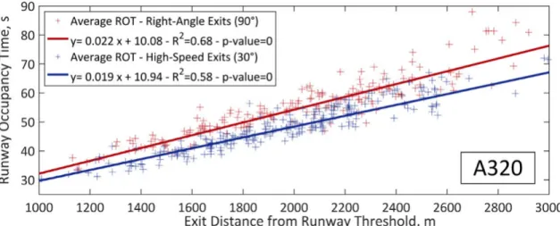
5-4 Evolution of A320 ROT depending on exit location and exit type . . . 39

5-5 Cumulative distributions of A320 ROT depending on the type of exit . . . 40

5-6 Cumulative distributions of A320 exit speed depending on the type of exit . . . 40

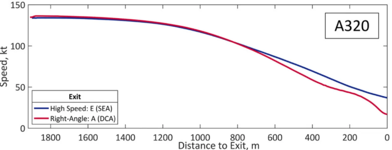
5-7 Example of similarly located high-speed (30°) and right-angle (90°) exits . . . . 41

5-8 Example of comparison of average A320 speed profiles for two similarly located high-speed (30°) and right-angle (90°) exits . . . 41

5-9 Example of comparison of average A320 deceleration profiles for two similarly located high-speed (30°) and right-angle (90°) exits . . . 42

5-10 Cumulative distribution of A320 ROT depending on airline . . . 42

5-11 Observed A320 ROT depending on approach speed . . . 43

5-12 Example of comparison of average A320 speed profiles for different final ap-proach speeds (exit K4, KPHL) . . . 44

5-13 Example of comparison of average A320 deceleration profiles for different final approach speeds (exit K4, KPHL) . . . 44

5-14 Contour plot of ROT depending on final approach speed and exit location for A320 using high-speed exits (30°) . . . 45

5-15 Contour plot of ROT depending on final approach speed and exit location for A320 using right-angle exits (90°) . . . 45

5-16 Example of arrival pressure categories at LaGuardia airport (KLGA) . . . 47

6-1 Overall prediction process of ROT . . . 50

6-2 Simplified functioning of a recurrent neural network . . . 52

6-3 Final architecture of the predictive model of exit use . . . 54

6-4 RNN training and validation loss depending on number of units . . . 55

6-5 General predictive process of mean/variance of ROT . . . 58

6-6 Validation loss of average ROT predictive model depending on number of units . 59 6-7 Distribution of mean squared error in the prediction of average ROT on testing dataset . . . 60

6-8 Example of predicted ROT distribution and weighted components per exit for an aircraft landing on runway 34L (KSLC) . . . 62

6-9 Predicted ROT distribution for runway 25L at Phoenix Sky Harbor International airport (KPHX) . . . 63

6-10 Predicted ROT distribution with larger left tail for runway 17 at Philadelphia International airport (KPHL) . . . 65

7-1 Runway configuration of Keflavík airport (BIKF) . . . 68

7-2 Aerodrome chart of Keflavík airport (BIKF) . . . 69

7-3 Example of flight tracks at Keflavík airport (BIKF on 01-01-2018) . . . 70

7-4 Example of the runway threshold and runway exit identified for a landing flight at Keflavík airport (BIKF) . . . 70

7-5 Distribution of wind at Keflavík airport (BIKF) . . . 72

7-6 Distribution of temperature at Keflavík airport(BIKF) . . . 72

7-7 Observed fleet-mix of landing aircraft at Keflavík airport (BIKF) . . . 72

7-8 Average daily distribution of landings at Keflavík airport (BIKF) . . . 73

7-9 Terminal locations for aircraft landing at Keflavík airport (BIKF) . . . 73

7-10 Runway Occupancy Time distribution at US airports and during peak-hours at Keflavík airport (BIKF) . . . 74

7-11 Exit system of runway 28 . . . 77

7-12 Potential new exit system for runway 28 . . . 79

7-13 Average Runway Occupancy Time of runway 28 depending on new high-speed exit location . . . 79

LIST OF FIGURES 11

7-14 Potential new exit system for runway 28 . . . 80

7-15 Average ROT of runway 28 depending on 2nd new high-speed exit location . . . 81

7-16 Exit system of runway 19 . . . 82

7-17 Potential new exit system for runway 19 . . . 84

7-18 Average Runway Occupancy Time of runway 19 depending on new high-speed exit location . . . 85

7-19 Exit system of runway 01 . . . 86

7-20 Exit system of runway 01 with planned taxiway . . . 88

7-21 Potential new exit system for runway 01 . . . 89

7-22 Average Runway Occupancy Time of runway 01 depending on new high-speed exit location . . . 90

7-23 Exit system of runway 01 with pilot incentive to exit early . . . 91

7-24 Average Runway Occupancy Time of runway 01 depending on new high-speed exit location with pilot incentive to vacate the runway early . . . 92

7-25 Exit system of runway 10 . . . 93

7-26 Potential new exit system for runway 10 . . . 95

7-27 Potential new exit system for runway 10 . . . 96

7-28 Average Runway Occupancy Time of runway 10 depending on new high-speed exit location . . . 96

7-29 Potential new exit system for runway 10 . . . 97

List of Tables

1.1 Legacy aircraft wake categories - FAA order JO 7110.65Y . . . 16

1.2 Final approach wake turbulence separation minima (IFR) - FAA order JO 7110.65Y 16

3.1 List of the 36 airports with available ASDE-X data . . . 24

3.2 Collected landing data, airport data and weather data . . . 30

5.1 Average A320 ROT for 7 airlines and 8 airports . . . 43

5.2 Average A320 ROT and exit location depending on arrival pressure for 26 airports 48

6.1 Parameters used by predictive models . . . 51

6.2 Example of sequence of input for an aircraft landing on runway 34L (KSLC) . . 53

6.3 Example of parameters of aircraft landing on runway 34L (KSLC) . . . 62

6.4 Example of runway exit system of runway 34L (KSLC) . . . 62

6.5 Example of exit use and ROT predictions for aircraft landing on runway 34L (KSLC) 62

7.1 Average Runway Occupancy Time for each runway at Keflavík airport (BIKF) . . 68

7.2 Collected landing data, airport data and weather data at Keflavík airport (BIKF) 71

7.3 Average Runway Occupancy Time during peak-hours for each runway at Keflavík

airport (BIKF) . . . 74

7.4 Legacy ICAO aircraft wake categories - ICAO DOC 4444 . . . 75

7.5 Final approach wake turbulence separation minima (IFR) - ICAO DOC 4444 . . 75

7.6 Average exit use and Runway Occupancy Time observed for each exit of runway 28 77

7.7 Average exit use and Runway Occupancy Time predicted for each exit of runway

28 . . . 78

7.8 Average exit use and Runway Occupancy Time predicted for each exit of runway

28 with additional high-speed exit . . . 80

7.9 Average exit use and Runway Occupancy Time predicted for each exit of runway

28 with a 2nd additional high-speed exit . . . 81

7.10 Average exit use and Runway Occupancy Time predicted for each exit of runway

28 with two simultaneously optimized additional high-speed exits . . . 82

7.11 Average exit use and Runway Occupancy Time observed for each exit of runway 19 83

7.12 Average exit use and Runway Occupancy Time predicted for each exit of runway

19 . . . 83

7.13 Average exit use and Runway Occupancy Time predicted for each exit of runway 19 with an additional high-speed exit . . . 85

7.14 Average exit use and Runway Occupancy Time observed for each exit of runway 01 86 7.15 Average exit use and Runway Occupancy Time predicted for each exit of runway 01 . . . 87

7.16 Average exit use and Runway Occupancy Time predicted for each exit of runway 01 with a bypassing taxiway . . . 89

7.17 Average exit use and Runway Occupancy Time predicted for each exit of runway 01 with new high-speed exit . . . 90

7.18 Average exit use and Runway Occupancy Time predicted for each exit of runway 19 with pilot incentive to vacate the runway early . . . 91

7.19 Average exit use and Runway Occupancy Time predicted for each exit of runway 01 with new high-speed exit and pilot incentive . . . 92

7.20 Average exit use and Runway Occupancy Time observed for each exit of runway 10 93 7.21 Average exit use and Runway Occupancy Time predicted for each exit of runway 10 . . . 94

7.22 Average exit use and Runway Occupancy Time predicted for each exit of runway 10 with new right-angle exit . . . 95

7.23 Average exit use and Runway Occupancy Time predicted for each exit of runway 10 with new taxiway and additional high-speed exit . . . 97

7.24 Average exit use and Runway Occupancy Time predicted for each exit of runway 10 with new taxiway and coupled high-speed exit . . . 98

7.25 Predicted reductions in average ROT with potential modifications . . . 98

A.1 List of aircraft used to develop predictive models . . . 109

B.1 Detailed performance of the predictive model of exit use . . . 111

C.1 Detailed performance of the predictive models of average ROT . . . 117

Chapter 1

Introduction

Motivation

Runway Occupancy Time (ROT) is one of the main elements limiting the throughput of runways at airports. Runway Occupancy Time can be formally defined as the "time interval between the aircraft crossing the threshold and its tail vacating the runway" according to Eurocontrol [1]. Under current regulations [2], the simultaneous occupancy of a runway by multiple landing airplanes is prohibited and an aircraft cannot be cleared to land if the previous aircraft has not vacated the runway. This rule limits the number of aircraft that can land on a runway on a given time period. A high average Runway Occupancy Time on a runway will considerably limit runway throughput. To prevent simultaneous runway occupancy, pilots are incentivized to vacate the runway as soon as possible [3] and air traffic controllers insure proper separations between aircraft on final approach as per Figure 1-1. These separations aim at leaving enough time for the leading aircraft to vacate the runway before the trailing aircraft reaches the runway threshold.

Figure 1-1: Interaction between Runway Occupancy Time and final approach separation

Current separations between aircraft on final approach are however mainly driven by wake-vortex turbulence. To reduce the risk of wake turbulence encounter on approach, strict sepa-ration minima are enforced and are usually more conservative than what Runway Occupancy

Time requires. These minima are based on categories of aircraft defined using the aircraft Max-imum Take-Off Weight (MTOW). Tables 1.1 and 1.2 present the aircraft legacy wake categories and final approach separation minima for IFR operations in application in the US.

Table 1.1: Legacy aircraft wake categories - FAA order JO 7110.65Y

Small Large B757 Heavy Super

MTOW (lb) MTOW ≤₄₁,₀₀₀ 41,000 < MTOW <300,000 B757 MTOW ≥₃₀₀,₀₀₀ A380, AN225

Table 1.2: Final approach wake turbulence separation minima (IFR) - FAA order JO 7110.65Y

Separation Minimum (NM) Following Aircraft

Super Heavy B757 Large Small

L eading _Aircraft Super MRS* 6 7 7 8 Heavy MRS* 4 5 5 6 B757 MRS* MRS* MRS* MRS* 4 Large MRS* MRS* MRS* MRS* 4 Small MRS* MRS* MRS* MRS* MRS*

*Minimum Radar Separation (2.5, 3 or 5NM)

In recent years, the US Federal Aviation Administration (FAA) and its European counterpart, Eurocontrol, have focused research efforts on reducing separation minima thanks to aircraft re-categorization programs (RECAT). These re-categorization programs have introduced more complex wake-turbulence classifications of aircraft based on both wingspan and MTOW leading to more aircraft categories and reduced separation minima on average. However, as wake vortex separation minima are reduced for aircraft on final approach, inter-arrival times are

progressively getting closer to the observed Runway Occupancy Time. This increases the

constraining impact of Runway Occupancy Time on runway throughput.

The average Runway Occupancy Time observed on a runway also drives the Minimum Radar

Separation (MRS) used on final approach. This Minimum Radar Separation can be equal

to 5.0, 3.0 or 2.5NM. According to ICAO PANS-ATM (Procedures for Air Navigation Services related to Air Traffic Management) [4], the Minimum Radar Separation may be reduced from 5.0 to 3.0NM if the radar capabilities enable it. An additional reduction to 2.5NM may be provided if 8 different conditions are fulfilled. These include observing an average ROT below 50s for a considered runway. By complying with the multiple requirements established by ICAO and reducing ROT below 50s, airport operators may reduce MRS and increase runway throughput.

The Runway Occupancy Time of a landing aircraft is the result of the aircraft braking perfor-mance in its landing environment. This braking perforperfor-mance enables the aircraft to potentially

17

vacate the runway after a specific braking distance where the aircraft reached an acceptable ground-speed. The main leverage airport operators have to reduce ROT consists in optimizing the exit system of runways. The exit system needs to be adapted to the expected landing operations. By designing runway exits with optimal parameters, airport operators can reduce the Runway Occupancy Time of aircraft and recover additional movement for their runways. The key exit parameters include the distance of the exits from the runway threshold and the

angle of the exits with the runway axis, ranging from 0◦ to 180◦. The most popular exit

an-gles are 90◦ (i.e. right-angle exits) and 30◦ (i.e. high-speed exits), depicted in Figure 1-2.

Compared to right-angle exits, high-speed exits are designed to enable aircraft to vacate the runway at a higher speed which reduces the braking distance on the runway. Finding optimal exit parameters is however difficult for airport operators as different aircraft types landing in different conditions can have very different braking behaviors.

Figure 1-2: Example of the two most popular runway exit angles

With the large amount of data on landing operations available today from surveillance systems, an opportunity exists to better understand the factors driving runway occupancy time and to design data-driven solutions to optimally locate runway exits and reduce ROT. Available data on landing operations includes large amounts of flight track data around airports (e.g. Airport Surface Detection data, ADS-B data), weather surface data and information on airport geometry and runway characteristics. By fusing multiple sources of data, a comprehensive picture of braking performance under various conditions can be obtained.

This thesis aims at leveraging operational data to analyze the roots of ROT and develop pre-dictive models of Runway Occupancy Time to optimize runway exit systems. A large volume of ROT measurements and associated landing parameters was first extracted from several data sources such as the Airport Surface Detection Equipment, Model X (ASDE-X) and the Automated Dependent Surveillance-Broadcast (ADS-B). These measurements were linked to weather and airport data derived from the Automated Surface Observing System (ASOS) and Google-Earth. Data-mining techniques were then applied to the collected data to identify precursors of Run-way Occupancy Time. A Random-Forest algorithm provided a ranking of landing parameters explaining the variance of ROT. The dominant factors influencing ROT were analyzed using ob-served speed and deceleration profiles on the runway. Based on this understanding, data-driven models were developed to predict Runway Occupancy Time. These models, based on

Recur-rent and Feed-Forward Neural Networks and trained on the collected data, give high-fidelity stochastic predictions of ROT for landing aircraft using a given set of available runway exits. At the runway level, by predicting ROT for thousands of landing flights with different landing parameters, runway-specific ROT probability distributions can be predicted. These models en-able the assessment of modifications to a runway exit system by evaluating their impact on the predicted ROT distribution. They were used to propose modifications to the exit system of an airport in Iceland showcasing a poor Runway Occupancy Time performance.

Research Objectives

The research objectives of this thesis can be summarized as follow:

• Develop data driven solutions to reduce Runway Occupancy Time by:

– Identifying and understanding factors driving Runway Occupancy Time using

flight-track data

– Developing predictive models of Runway Occupancy Time based on the identified

precursors

– Using the predictive models to optimize runway exit systems at capacity constrained

airports

Thesis Outline

This thesis is organized in the following manner. First, a literature review is presented in Chapter 2. Second, a methodology to extract Runway Occupancy Time measurements and exogenous landing data is introduced in Chapter 3. Chapter 4 presents a method used to identify the factors driving ROT. Fourth, a detailed analysis of the impact of each driving factor on Runway Occupancy Time is described in Chapter 5. Chapter 6 presents the methodology used to develop predictive models of Runway Occupancy Time and assess their performance. Finally, a case study on reducing Runway Occupancy Time at Keflavík airport (Iceland) by optimizing the runway exit system is presented in Chapter 7. Chapter 8 presents the conclusions drawn from this study.

Chapter 2

Literature Review

This thesis presents a data-driven approach to understanding and reducing Runway Occupancy

Time at capacity-constrained airports. Runway Occupancy Time has been identified as a

potential limitation to runway throughput more than 60 years ago and several studies have

focused on identifying factors driving Runway Occupancy Time. Several approaches were

developed as well to model Runway Occupancy Time and be able to propose runway exit systems minimizing the Runway Occupancy Time of landing aircraft. This section presents a comprehensive review of the different research efforts aiming at understanding and modelling Runway Occupancy Time.

2.1

Understanding Factors Driving Runway Occupancy Time

Several studies have been conducted in the past to identify the factors influencing Runway Occupancy Time. They used various collection methods to obtain ROT measurements and conduct statistical analysis.

Some of the first studies of Runway Occupancy Time date back to the 1980s to identify potential limitations at reducing separations between aircraft on final approach. The MITRE corporation was tasked by the FAA to study the interaction between inter-arrival times and ROT and needed to understand the variability of ROT depending on multiple factors. Using data collected by visual means between 1972 and 1973 at 6 US airports, Koenig [5] identified that Runway Occupancy Time was not solely driven by braking performance but also influenced by pilot motivational factors. These motivational factors were driving the choice of the exit used to vacate the runway and encompassed the time to gate, airline-specific procedures and traffic density for instance.

In 1983, additional studies of ROT were funded by the FAA. As a contractor, the MITRE cor-poration collected 1755 Runway Occupancy Time measurements at LaGuardia airport (KLGA), Newark airport (KEWR) and Boston Logan International airport (KBOS). These measurements

were obtained by visually observing multiple landings from the control tower. Using this data, the Runway Occupancy Time dependence on the wake category of the landing aircraft and the observed runway condition (dry/wet) was analyzed by Weiss and Barrer [6]. It was found that the runway condition had a relatively small impact on Runway Occupancy Time. The data used for this study was however limited to a few airports and not highly reliable due to the difficulty of measuring ROT from the control tower. The main difficulty encountered was to reliably measure the time when the aircraft was crossing the runway threshold and vacating the runway from the control tower.

This difficulty was overcome by NASA in 1999 with the development of the Dynamic Runway Occupancy Measurement System (DROMS). Using mode-S transponders and multilateration, precise aircraft position could be collected at Atlanta Hartford International airport (KATL) and Runway Occupancy Time measurements could be calculated. Lee et al. [7] used this system to collect more than 3000 ROT measurements at Atlanta during 15 days and analyze factors influencing ROT. They found that ROT was equally influenced by the approach speed and weight of the aircraft, barely influenced by winds observed on approach and increased by less than 5% with wet runway conditions versus dry conditions. It was also observed that ROT was not dependent on the airline, contradicting MITRE previous findings.

More recently, the collection of Runway Occupancy Time measurements was eased by the avail-ability of modern detection systems around airports. The Airport Surface Detection Equipment - Model X (ASDE-X) was installed by the FAA at 36 US airports starting in 2004 and provided a large amount of data regarding flight tracks around airports. In 2009, Kumar, Sherry, and Kicinger [8] were the first to leverage this data to analyze Runway Occupancy Time. They developed a simple method to extract ROT measurements from ASDE-X data and collected 2035 Runway Occupancy Time measurements at Dallas Fort Worth airport (KDFW). Kumar, Sherry, and Kicinger [8] used this data to analyze the correlation of ROT with the momentum of landing aircraft.

ASDE-X flight track data was also used by Kolos-Lakatos [9] in 2013 to understand the interaction

between Runway Occupancy Time and Wake Vortex separation. ROT data was collected

at Boston Logan airport (KBOS), LaGuardia airport (KLGA), Newark airport (KEWR) and Philadelphia airport (KPHL) by modelling runways as polygons and computing the time each landing aircraft spent in the runway polygon. Using numerous ROT measurements, Kolos-Lakatos [9] studied the dependency of ROT with the aircraft size, the type of runway exit used and IMC/VMC weather conditions. It was found that ROT generally increases with the size of the aircraft although small aircraft sometime had a similar ROT to large aircraft due to the optimization of exits for larger aircraft. Runways equipped with high-speed exits (30°) were also observed to have a lower Runway Occupancy Time. Finally, no significant difference was observed regarding the ROT of aircraft landing in IMC conditions and VMC conditions. The studies conducted so far to analyze Runway Occupancy Time highlighted the influence of specific factors on Runway Occupancy Time. They were however limited to a few airports in the US and based on a limited set of Runway Occupancy Time measurements. They also

2.2. MODELLING RUNWAY OCCUPANCY TIME 21

focused on specific factors that could influence Runway Occupancy Time and were sometimes contradictory. An opportunity exists today to use the large amount of flight track data available around airports in the US to conduct a system level analysis of the factors driving Runway

Occupancy Time. Collected data regarding landing aircraft would need to encompass all

potential factors that could influence Runway Occupancy Time to get a full picture of ROT precursors and assess their relative importance.

2.2

Modelling Runway Occupancy Time

Based on the understanding of factors driving ROT, built over time, multiple models have been developed in the past to optimize the exit system of runways to reduce ROT.

Horonjeff et al. [10] were the first to develop a probabilistic method to optimally locate runway exits in 1959. The braking distance and time needed by an aircraft type to reach a specific ground speed were modelled by a joint probability distribution. Using this joint probability distribution, the model solved an optimization problem to find the exit locations providing the lowest go-around probability given the observed fleet-mix and separations on final approach at the airport. Daellenbach [11] improved this model in 1974 using dynamic programming to solve the optimization problem.

In 1990, Ruhl [12] proposed a new method to design optimally located runway exits by mod-elling the deceleration of aircraft on the runway. These models broke-down the landing phase in multiple sub-phases of deceleration described by a finite number of parameters. The dis-tributions of these parameters were obtained using 180 video records of aircraft landing at 4 airports in the US. The impact of multiple landing factors on these parameters was assessed

using statistical analysis. For each landing aircraft, the model computed the speed of the

aircraft at each runway exit and compared it to the exit acceptance velocity. The first exit with an exit acceptance velocity higher than the speed of the aircraft was assumed to be used by the aircraft to vacate the runway. The model then assumed that the aircraft would have adjusted its deceleration to reach the exit at the acceptance velocity and predicted a Runway Occupancy Time value. In the end, the model would predict the Runway Occupancy Time and exit use of a landing aircraft given its aircraft type, airline, final approach speed and multiple environmental conditions. By using a Monte-Carlo simulation, optimal exit locations could then be investigated for a specific airport.

In 1993, Hobeika et al. [13] used a similar approach to create the Runway Exit Design Interac-tive Model (REDIM). This tool modeled the deceleration of a landing aircraft on the runway for 4 different categories of aircraft. The landing phase was broken-down in five different

deceleration sub-phases described by a set of kinematic equations and parameters. These

different parameters were calibrated using both simulation and collected ROT data at US air-ports. The braking phase and flare phase were represented as random events to stochastically model deceleration. Using this decomposition of deceleration, the model could predict the mean and variance of the landing distance and ROT required by an aircraft to reach a specific

exit speed. Using these predicted values, constraints regarding exit location could be derived for each aircraft type. These constraints were used to design an optimization problem solved using dynamic programming to find a set of exits minimizing the average ROT for an observed fleet-mix.

This model was improved successively over the years and used by the FAA to modify the runway exit system of major US airports. Changes included the addition of new parameters in the modelling of Runway occupancy Time such as the weight of the landing aircraft and more flexibility in the recommendation of optimal exit locations. Both of these changes were implemented in the second version of the model by Trani et al. [14]. In 1995, Gu, Trani, and Zhong [15] modified the model to account for the impact of gate location on the choice of the exit used to vacate the runway. This was done by either adapting the assumed deceleration rates or assigning exits minimizing Runway Occupancy Time plus the weighted taxi-time to gate to the landing aircraft. A third version of the model is planned and will use ASDE-X data to better estimate kinematic parameters and will propose aircraft-specific modelling.

In 2007, Barbas, Vázquez, and López [16] proposed an alternative approach to model Runway Occupancy Time and assess changes to runway exit systems. Their approach consisted in using a two-step predictive model combined with a Monte-Carlo simulation to get an estimate of the average ROT of a runway. Predictions of exit use and Runway Occupancy Time were made for thousands of landing aircraft to obtain this average estimate. For each landing aircraft, the probabilities of use of the different available exits were first predicted using a logistic regression. Then, an exit was assigned to the aircraft, sampled at random from the predicted distribution of exit use. Given this exit, the ROT of the aircraft was predicted by modelling the speed profile of the aircraft on the runway using a non-linear speed function. The exit system of a runway could then be optimized by assessing the impact of potential modifications on the predicted average ROT. The different models were calibrated using 1550 ROT measurement collected at Madrid Barajas airport (LEMD) using visual observations.

Since 1959, multiple predictive methods have been designed to optimize runway exit systems and reduce Runway Occupancy Time. They mostly consisted in modelling Runway Occupancy Time and exit usage. Their performance and complexity have increased over time, accounting for more and more factors impacting Runway Occupancy Time. These methods were based on the modelling of the deceleration of aircraft on the runway and were calibrated using small sets of landing observations. The advent in recent years of advanced supervised machine-learning algorithms, able to model non-linear phenomenon, gives the opportunity to develop new predictive methods of Runway Occupancy Time. These methods would not require making assumptions on the braking physics of landing aircraft while still providing a high predictive performance. The large amount of operational data available today could be used to develop such models. These models could be leveraged to optimize runway exit systems at capacity-constrained airports.

Chapter 3

Runway Occupancy Time Data

Collection using Landing Data

To analyze the roots of Runway Occupancy Time and propose data-driven solutions to reduce ROT at airports, a significant amount of Runway Occupancy Time measurements around major US airports were first collected. These measurements were extracted based on landing flight tracks at 36 US airports. Landing parameters and deceleration information associated to each ROT measurement were gathered as well to understand the influence of several factors on ROT. This section presents the methodology used to collect a significant amount of Runway Occu-pancy Time measurements around major US airports and the associated landing parameters and deceleration information.

3.1

Runway Occupancy Time Measurements

To gather Runway Occupancy Time measurements, Airport Surface Detection Equipment -model X (ASDE-X) data was collected from 36 major US airports listed in Table 3.1 between March 2015 and April 2016. Additional ASDE-X data regarding A320/A321 NEO and B737 MAX 8/9 aircraft observed in 2018 at the same airports was gathered as well and used solely to develop the predictive models of ROT, described in Section 6. The Airport Surface Detection Equipment - model X is a detection system, implemented progressively since 2003 around major US airports, and fusing data from multiple sources such as ADS-B receivers, surface surveillance radar, airport surveillance radars, terminal automation system and multilateration sensors [17]. The system is used by tower controllers to visualize airport operations and aircraft movements in real-time. The collected data includes raw flight tracks of departing and arriving aircraft detected within a 10NM radius around each airport. Each flight track is composed of position parameters (latitude, longitude and sea-level altitude) and kinematic parameters (ground speed) sampled at a rate of one second and also includes general aircraft identification parameters such as the aircraft type, the airline and the callsign of the aircraft.

Table 3.1: List of the 36 airports with available ASDE-X data

KATL KBDL KBOS KBWI KCLT KDCA KDEN KDFW KDTW

KEWR KFLL KHOU KIAD KIAH KJFK KLAS KLAX KLGA

KMCO KMDW KMEM KMIA KMKE KMSP KORD KPHL KPHX

KPVD KSAN KSDF KSEA KSFO KSLC KSNA KSTL PHNL

Additional data was collected regarding runway characteristics at the 36 airports using the 28-Day NASR Subscription Aeronautical Data from the FAA, effective October 12, 2017 [18]. This source of data gives up-to-date runway information such as displaced runway threshold coordinates, runway width, length or pavement description. Information regarding runway exits, existing in 2015, was also gathered manually based on airport diagrams and geospatial data extracted from Google Earth. For each runway of the 36 airports, the coordinates and angle of each runway exit were measured as per Figure 3-1. Information regarding at total of 4442 exits corresponding to 284 runways was obtained. Finally, the length from nose to tail of 504 common aircraft types observed in the National Airspace System (NAS) was collected using data from the FAA aircraft characteristics database [19], aircraft manufacturer websites and the skybrary aircraft database [20].

Figure 3-1: Example of runway exit measurements (KATL, exit SG14)

To extract ROT measurements from the different ASDE-X flight tracks, some data-processing was required. This data processing, presented in the following part is generic and was applied to flight tracks obtained using various data sources such as ASDE-X or ADS-B.

First, the different flight tracks needed to be distinguished from each other. Based on the track identification numbers, a first set of separate flights tracks was identified. These flight tracks were then sub-divided to create a new set of refined flight tracks by identifying successive data-points separated by more than ten minutes. This enables the separation of successive flights for aircraft with the same track identification number.

3.1. RUNWAY OCCUPANCY TIME MEASUREMENTS 25

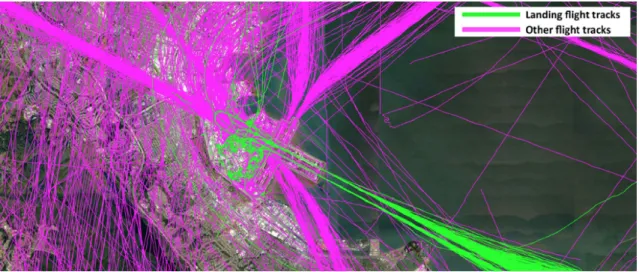
using a set of logical rules. A flight track corresponded to a landing flight when the initial broadcasted ground speed was higher than 80kt and when the aircraft was flying below a 100ft AGL (Above Ground Level) at some point during its flight. These two thresholds were chosen based on repeated trials to identify most of the landing aircraft using flight tracks visualisation. An example of the landing flight tracks identified at San Francisco airport (KSFO) on 04-01-2015 using this separation process is depicted in Figure 3-2.

Figure 3-2: Example of the identification of landing flights at San Francisco airport (KSFO on 04-01-2015)

Third, the runway used for landing was identified for each flight track corresponding to a landing flight. During the first 10 seconds when the aircraft flew below 50ft AGL, its distance to each of the displaced runway thresholds of the airport was computed. The runway used for landing corresponded to the threshold associated to the minimum computed distance, as each aircraft is flying straight above it during landing.

Fourth, based on the Eurocontrol definition of ROT [1], two timestamps needed to be computed to measure ROT. These timestamps correspond to the time when the aircraft flew above the

runway threshold t0 and the time when its tail vacated the runway tend. While the first

timestampt0was simply identified based on the closest point of the flight track to the displaced

runway threshold, the process used to identify the second timestamptendis more complex. It

was assumed that the aircraft position coordinates, recorded by the detection system (ASDE-X or ADS-B), corresponded to the GPS antennas of the aircraft, usually located around the center of modern jet aircraft. Based on this hypothesis, the tail of the aircraft is assumed to be clear of the runway when the distance between the center of the aircraft and the runway boundary is more than half the length of the aircraft projected on a perpendicular axis to the runway. This projected tail length can be computed using Equation 3.1 and is depicted in Figure 3-3.

D =sin(α) ∗ L

2 (3.1)

withα the angle of the runway exit and L the total length of the aircraft

Figure 3-3: Example of projected tail length of aircraft using exit SG14 (KATL)

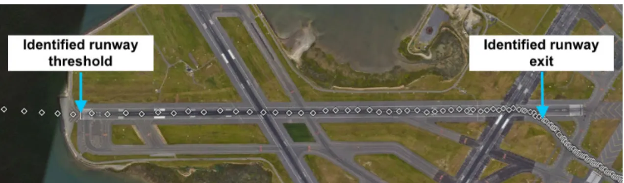
This criteria was used to identifytend. The exit used to vacate the runway was first identified

to get access to the angle of the exit. The distance between the center of the aircraft and the

runway centerline was computed successively for all the points followingt0. When this distance

was more than half the runway width, the distance between the aircraft and each of the exits of the runway was computed and the closest runway exit was assumed to be used by the aircraft to vacate the runway. Figure 3-4 shows the runway threshold and runway exit identified for a given landing flight at Boston Logan International airport (KBOS).

Figure 3-4: Example of the runway threshold and runway exit identified for a landing flight at Boston Logan International airport (KBOS)

Second, the projected tail length of the aircraft was computed by projecting half of the length of the aircraft to an axis perpendicular to the runway using the exit angle. The distance between the center of the aircraft and the runway centerline was compared to the projected tail-length

for all the points followingt0. When this distance was higher than the projected tail-length plus

half the runway width, the tail of the aircraft was assumed to be cleared of the runway boundary

andtend was identified. The Runway Occupancy Time was then measured by computing the

3.1. RUNWAY OCCUPANCY TIME MEASUREMENTS 27

Finally, values of ROT less than 20 seconds were dismissed. These values usually corresponded to poor quality flight track data with unreliable values of position, speed or altitude. In total, 3,446,460 Runway Occupancy Time measurements with a 1 second precision were extracted from ASDE-X flight tracks at the 36 airports. The overall process used to extract ROT measure-ments from flight tracks is summed-up in Figure 3-5.

Flight track data

Yes No Initial aircraft ground speed > 80Kt? Idenfitication of unique track numbers Identification of successive points separated by  more than 10min

Distinct flight tracks 

Yes

No Aircraft flying below 100ft AGL

 at some point? Landing flight tracks

Other flight tracks

Runway Data from 28-Day NASR subscription (threshold coordinates, runway width) 

Identification of closest runway threshold

during first 10s below 50ft AGL Landing flight tracks with

identified runway used

Identification of closest point to threshold &

1st _{point outside of} runway boundary

Identification of closest exit to 1st point outside

runway boundary

Computation of Runway Occupancy

Time

Runway exit Data (coordinates and angle)

Aircraft length Data

Is Runway Occupancy  TIme > 20s?

Runway Occupancy Time Measurements

Dismissed ROT measurements associated to low quality

flight track Data

3.2

Determining Deceleration Information and Landing

Parame-ters

For each landing flight, additional data characterizing the landing was collected. First, the aircraft type (i.e. ICAO aircraft code), airline and final approach ground speed of the aircraft were gathered. The final approach ground speed of the aircraft corresponds to the aircraft

ground speed above the runway threshold (t0). Data was also gathered regarding the runway

exit used to vacate the runway and more specifically its distance from the runway threshold and its angle. It was suspected that the presence of another aircraft following on final approach might have an influence over ROT. For each landing flight, information about the number of following aircraft detected on approach was collected. The type of the first following aircraft and its distance from the landing aircraft when crossing the runway threshold were also extracted. An example of a leading and trailing aircraft on final approach at Atlanta Hartsfield airport (KATL) and the computed distance between them is depicted in Figure 3-6.

Figure 3-6: Example of leading and following aircraft at Atlanta Hartsfield airport (KATL)

The observed weather during landing could have an impact on Runway Occupancy Time. Weather parameters (temperature, wind, visibility, day/night indicator, pressure altitude, type and amount of precipitation) were collected at 5-minute time intervals at each airport using ASOS (Automated Surface Observing System) data archives and temporarily linked with the

identified landing observations att0. More than 900 ASOS weather stations have been installed

in the US since 1991 and are managed by the National Weather Service (NWS), the Federal Aviation Administration (FAA) and the Department of Defense [21]. They are mostly used to assess surface weather for aviation purposes around airports. Data is recorded every 1 or 5 minutes depending on the gathered weather information and is available online [22]. General flight conditions (VMC/IMC) were derived from the visibility and ceiling data provided by ASOS data archives and also obtained from the FAA Aviation System Performance Metrics (ASPM) data service.

Information was also gathered regarding the braking performance of each aircraft. The ground

speed of each landing aircraft was collected from the runway threshold crossing (t0) to the

moment the aircraft vacated the runway (tend). The ground speed profiles, corresponding to

3.2. DETERMINING DECELERATION INFORMATION AND LANDING PARAMETERS 29

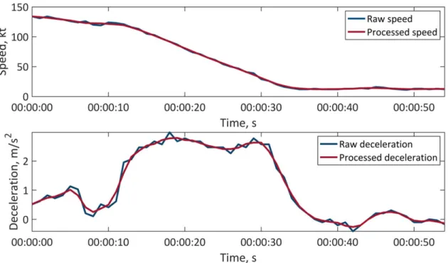
speed data points of each profile were re-sampled to be regularly spaced in time (i.e. every

second). Duplicates were removed and the speed profiles were smoothed using a moving

average filter with a 5s span. Deceleration profiles were then derived by differentiating the smoothed speed profiles. An example of the speed and deceleration profiles obtained using this process is depicted in Figure 3-7. The collected speed and deceleration profiles were used later to understand the impact of certain parameters on the braking performance of aircraft and therefore on Runway Occupancy Time.

Figure 3-7: Example of speed and deceleration profiles of an A320 landing at Charlotte Douglas Inter-national airport (KCLT)

Finally, data was collected regarding the location of the gates reached by aircraft after landing. The last recorded ASDE-X coordinates for each landing aircraft were used as a surrogate for gate location. For approximately 99% of the landing flights, these coordinates corresponded to the gate location. In nearly 1% of the cases, however, they did not seem to correspond to a gate location and the ASDE-X system stopped too early recording data. This might be due to the pilot switching-off the transponder of the aircraft after landing. An example of the last coordinates of each landing flight track recorded at Honolulu airport (PHNL) is depicted in Figure 3-8. These coordinates were used to compute the distance between the runway exit used by each aircraft to vacate the runway and its terminal gate. They were also used to assess whether the runway exit was on the same side as the final gate location relatively to the runway axis. This data, regarding the gate location, was used solely for the the development of the predictive models of ROT detailed in Chapter 6.

Figure 3-8: Example of recorded gate locations at Honolulu International airport (PHNL)

In the end, the database was composed of 3,446,460 aircraft landing observations at 36 airports, described by 23 discrete parameters and by their associated speed and deceleration profiles on the runway. These parameters, listed in Table 3.2, are meant to encompass the main factors that could drive Runway Occupancy Time under normal braking conditions.

Table 3.2: Collected landing data, airport data and weather data

Landing Data Airport Data Weather Data

• Runway Occupancy Time • Aircraft type • Airline • Approach speed • Number of following aircraft

• Following aircraft type • Distance of the

following aircraft • Speed profile on the

runway

• Deceleration profile on the runway

• Airport • Runway used

• Location of the runway exit used

• Angle of the runway exit used

• Distance between the runway exit used and the gate location • Relative position of the

runway exit used with the runway axis and the gate location

• Day/night indicator • Temperature • Headwind • Crosswind

• VMC/IMC conditions (based on airport operating mode) • VMC/IMC conditions 2 (based

on measured visibility and ceiling)

• Type of precipitation • Amount of precipitation • Pressure altitude • Visibility

Chapter 4

Identifying Factors Driving Runway

Occupancy Time

The landing data, described in Chapter 3 was used to identify factors driving Runway Occupancy Time1. The following section first analyzes the variability of ROT observed in the landing data before presenting the method used to identify the factors driving ROT and its results.

4.1

Analyzing the Variability of Runway Occupancy Time

According to Figure 4-1, depicting the cumulative distribution of ROT measured at the 36 US airports, a large variability in Runway Occupancy Time measurements was observed in the landing data. While aircraft spend on average 49s on the runway, 95% of ROT values are encompassed between 34s and 74s. The observed ROT variability at the system level is due to various ROT performances among airports and a significant ROT variability within each airport.

Figure 4-2, depicting the cumulative distribution of ROT for each of the 36 airports, shows that airports such as Ronald Reagan Washington National Airport (KDCA) have a relatively low ROT (40s median ROT) while other airports such as Honolulu International Airport (PHNL) perform poorly in terms of ROT (57s median ROT). According to this figure, variability in Runway

Occupancy Time is also observed within each airport. At Dallas Fort-Worth International

airport (KDFW), for instance, Runway Occupancy Time ranges from 36s to 73s (95% of the values). The variability in Runway Occupancy Time, observed at several scales, is driven by multiple factors that collectively impact the braking deceleration of aircraft.

1To analyze ROT, a very-conservative filtering of extreme ROT values was done by identifying landing observa-tions in the database with an ROT more than 3 scaled Median-Absolute-Deviaobserva-tions (MAD) away from the median ROT per aircraft type and runway. This method is detailed in [23]. These extreme values representing less than 3% of the data correspond to abnormal braking behavior on the runway

Figure 4-1: Cumulative distribution of ROT at the system level (36 US airports)

Figure 4-2: Cumulative distributions of ROT for the 36 US Airports

4.2

Identifying Factors Driving ROT using a Random Forest

Algo-rithm

To identify the factors driving Runway Occupancy Time, a random-forest regression algorithm was trained to predict Runway Occupancy Time using the landing database. A random-forest is made of an ensemble of decision trees, trained to fulfill a regression or classification task. It usually provides a high predictive power while being relatively resilient to over-fitting and easy to tune. This supervised learning algorithm, if trained on a regression task, can provide a ranking of the importance of each input factor in explaining the variance of the predicted target variable in a dataset. This capability is often leveraged in data-science settings to identify the most important features to include in more complex predictive models (i.e. feature selection). The ranking is based on the relative appearance of the difference factors in the nodes of each decision tree and the ability of each node to reduce variance. By training a random-forest to predict ROT, a ranking of the different factors based on their ability to explain the variance of ROT can be therefore obtained.

4.2. IDENTIFYING FACTORS DRIVING ROT USING A RANDOM FOREST ALGORITHM 33

4.2.1

Random Forest Models

The random-forest algorithm, first introduced in 1995 [24], is a bootstrap-aggregating (i.e. bag-ging) ensemble algorithm. Random-forest algorithms are used for both non-linear regression and classification tasks. They rely on building a forest of decision trees to fulfill a prediction task. In a regression setting, the different trees are trained using a dataset made of observed target values and potential predictors. The overall process used to build a random forest model is depicted in Figure 4-3. For each tree, the original dataset is resampled at random with replacement to create a bootstrapped dataset used to train the tree on the prediction task. The different trees are then used together to make collective predictions by averaging predictions. The different trees are weak-learners as they have seen only part of the original dataset. They have however a great prediction capability together and can account for a great proportion of the variance observed in target values.

Resampled Dataset 1 Input Parameters Bootstraped Datasets Successive Randomized Optimal Splits Training Dataset Tree 1

... Resampled Dataset t Resampled Dataset T

... Tree t Tree T

Figure 4-3: Training process of a random-forest algorithm

Each tree in the forest is made of nodes splitting the input data in two, based on the value of a decision factor. This decision factor can be either a categorical variable or a numerical variable. If the variable is categorical, the data is split in two by diving the variable in two sets of categories. If the variable is numerical, the data is split in two using a splitting value. During the training process, these variables and splitting values or sets of categories are chosen for each node successively based on their ability to decrease the variance of target values for the created sub-datasets. An additional randomness is added in the training process by allowing the algorithm to choose the node variable from a restrained set of variables selected at random. Each tree is thus built progressively by making randomized optimal variable choices and splits.

To optimize the performance of a random-forest model, a set of hyper-parameters need to be tuned. These hyper-parameters encompass the number of trees in the forest and the maximum

depth of each tree. The performance of the model usually scales-up with the number of trees and is capped by computing power while the maximum depth has an impact on the complexity of each tree.

Once a random-forest algorithm has been trained to fulfill a regression task, a ranking of the different factors based on their ability to reduce the variance of the dataset can be computed. By looking at how much each node of each tree contributed to decrease the total variance of the dataset, a percentage of explained variance can be attributed to each factor. First, a decrease of variance can be attributed to each node of a tree based on equation 4.1.

∆V ar(i) = Var(i) − pl·V ar(il) −pr ·V ar(ir) (4.1)

with: ∆V ar(i)the decrease in variance provided by node i

V ar(i)the variance observed in the dataset split at node i

V ar(il)the variance observed in the left dataset resulting from the split

V ar(ir)the variance observed in the right dataset resulting from the split

pl the proportion of the population of the left dataset resulting from the split

pr the proportion of the population of the right dataset resulting from the split

Second the contribution of each factor to the reduction of variance is computed using equation 4.2. C(X ) = _N1 T Õ t ∈T Õ i ∈t |s(i)=X p(i) · ∆V ar(i) (4.2)

with: C(X )the contribution of factor X to the reduction of variance

NT the number of trees

T the forest of trees

t a given tree in the forest

∆V ar(i)the decrease in variance provided by a node i in a tree t

p(i)the proportion of the population reaching node i

s(i)the factor used to split data at node i

The contribution of each factor can be then scaled and understood as the percentage of ex-plained variance that can be attributed to a specific variable. Further details about random-forest algorithms and the ranking method are presented in [25]. The following section explains how such a ranking can be obtained for Runway Occupancy Time.

4.2.2

Training a Random Forest Algorithm to Predict ROT

To obtain a ranking of the factors driving the variance of Runway Occupancy Time, a random-forest algorithm was trained to predict ROT using the landing data. A training set was first sampled from the filtered collected landing data and composed of 450,000 landing observa-tions. These landing observations are described by the various recorded parameters, listed

4.2. IDENTIFYING FACTORS DRIVING ROT USING A RANDOM FOREST ALGORITHM 35

in Table 3.2 (except parameters regarding the gate location, the airport, the runway used and the speed and deceleration profiles). The parameters describing each landing were used as predictors to train a random-forest model to predict ROT. No significant preprocessing of numerical features was required due to the flexibility of random-forest algorithms regarding standard-scaling. Categorical variables were encoded by mapping categories to integers. This enables the random-forest model to partition categorical variables into subsets of categories in the nodes. Categories with less than 20 observations were also pooled in a common single category (named "other") for each categorical feature for computational efficiency.

The training set was used to tune the hyper-parameters of the random-forest algorithm such as the number of trees and the maximum depth of each tree. These hyper-parameters were chosen in order to minimize the mean squared error (MSE) on the prediction of ROT using a 3-fold cross-validated grid-search. Random-forest models with 50 to 300 trees with a maximum depth ranging from 5 to 25 were tested. The maximum depth of each tree was found to have the most impact on the cross-validated mean-squared error while the number of trees had a minor impact. It was found that a forest made of 300 trees of maximum-depth 25 provided the best performance given the available amount of computing power. A model with these

hyper-parameters was trained on the full training set and reached a 24s2 mean squared error

(MSE) in the prediction of ROT on a testing dataset made of 50,000 other randomly selected landing observations. The open source python H2O package was used to train and build the forest algorithm [26]. A non-representative example of a tree built by the random-forest algorithm and truncated to a depth of 5 is depicted in Figure 4-4.

Aircraft Type Exit Location < 2115m 148 levels Exit Location < 2238m 88 levels Aircraft Type < Exit Location < 2596m >= Aircraft Type < Exit Location < 2688m >=

Following Aircraft Type 44 levels

Angle < 41° 104 levels

Final Approach Speed < 138kt <

Angle < 60° >=

Temperature < 59F 44 levels

Final Approach Speed < 10kt 44 levels

Temperature < 67F <

Following Aircraft Type >= 43.9s 153 levels 45.7s 65 levels 45.8s < 49.2s >= 59.5s < 54.4s >= 68.4s < 77.9s >= 52.2s < 50.5s >= 1041.0s < 55.6s >= 68.2s < 64.2s >= 83.9s 170 levels 92.1s 46 levels

4.3

Ranking the Factors Driving ROT

By looking at how much each node of each tree of the random-forest model contributed to decrease the total variance of the training dataset, a ranking of the importance of each factor in the estimation of ROT was determined. This ranking, presented in Figure 4-5, lists the percentage of explained ROT variance that can be attributed to each factor.

4 9 .3 % 1 1 .1 % 1 0 .7 % 6 .8 % 6.1 % 3.4 % 2 .2 % 1 .8 % 1 .6 % 1.5 % 1 .4 % 1.3 % 0 .9 % 0 .6 % 0 .6 % 0 .3 % 0 .3 % 0 .1 % 0% 10% 20% 30% 40% 50% 60% Ex it Lo cati o n A ir cr af t T yp e Ai rl in e Ex it A n gl e Fi n al A p p ro ac h Sp eed Fol lo w ing A ir cr af t Ty pe Tem p er at u re D ay /Ni gh t He ad W in d Cr o ss W in d P re ss u re A lt itu d e D is ta n ce o f th e Fo llo w er Ty p e o f P rec ip itat io n Vi si b ili ty Nu m b er o f Fo llo w er s V MC /I MC VMC /I MC 2 A m o u nt o f P re ci p itat io n P e rc e nt ag e o f Ex pl ai ned RO T V ar ianc e Dominant factors (87.4%)

Figure 4-5: Ranking of the importance of ROT factors

In this ranking, the exit used by the landing aircraft to vacate the runway appears to be dominant and accounts for 56.1% of the explained variance of ROT. A runway exit can be characterized by its distance from the runway threshold, also called exit location (accounting for 49.3% of the variance) and by its angle with the runway axis (accounting for 6.8% of the variance). The aircraft type and final approach speed also appear to have a significant impact on ROT (accounting respectively for 11.1% and 6.1% of the variance). More surprisingly, the airline is the third most important ROT factor (accounting for 10.7% of the variance). This contradicts previous studies that did not observe significant differences in ROT between carriers [7]. The presence of one or more following aircraft on final approach also impacts

ROT and accounts for 5.3% of the variance. Finally, weather factors appear to have less

influence over ROT individually but account together for 10.7% of the ROT variance. It can be noted that some factors are correlated such as the airline and aircraft type. Their collective influence on ROT variance is usually divided evenly among the different factors thanks to the randomness implemented in the tree splits. Factors explaining more variance might get however an increased credit in some cases. In the end, 87.4% of the explained variance can be attributed to only 5 dominant factors. The impact of these dominant factors on Runway Occupancy Time needed to be understood and a detailed analysis of their relative influence is presented in the following section.

Chapter 5

Understanding the Impact of

Dominant ROT Factors

The ranking of ROT factors provided by the random forest algorithm identified five dominant factors that account for 87.4% of the variance of Runway Occupancy Time. Indeed, the runway exit (location and angle), the airline, the aircraft type, the approach speed and the type of the following aircraft on approach almost completely explain the variance of ROT. An analysis of the impact of the five mentioned factors on ROT is presented in this section. This analysis was based on the same filtered landing data from 36 airports. The analysis focuses first on the general impact of aircraft type on ROT before analyzing the influence of the four other factors for the specific case of Airbus A320s.

5.1

Analysis of the Impact of Aircraft Type

According to the ranking of ROT factors, presented in Figure 4-5, the aircraft type accounts for 11.1% of the variance of ROT. Figure 5-1 shows the cumulative distributions of ROT for aircraft of each wake category ("Small", "Large", "757", "Heavy" and "Super Heavy"). It appears that the distributions of Runway Occupancy Time differ between legacy wake vortex categories and that aircraft belonging to categories with a higher maximum take-off weight (MTOW) have a higher Runway Occupancy Time on average.

Even within each wake category, specific aircraft models have different ROT distributions. This is illustrated in Figure 5-2 which shows the cumulative distributions of ROT for 6 common aircraft types belonging to the “Large” category. Within the B737 and A320 families, the largest aircraft variants (A321 and B737-900) have a higher Runway Occupancy Time compared to smaller versions. These larger aircraft variants differ not only by their heavier MTOW but also by their higher approach speeds due to tail clearance requirements. A higher MTOW and approach speed increases the momentum of the aircraft which results in higher ROT.

Figure 5-1: Cumulative distributions of ROT per wake category

Figure 5-2: Cumulative distributions of ROT for 6 common “Large” aircraft types

Because of the high dependency of ROT with the type of aircraft, the influence of other factors on ROT must be analyzed by looking at specific aircraft types. This study presents a focused analysis on the A320 aircraft type, relatively well represented at each of the 36 studied airports with 255,376 extracted landings.

5.2

Analysis of the Impact of the Runway Exit Used

The runway exit that is used by an aircraft to vacate the runway accounts for 56.1% of the variance of ROT. The population of runway exits at US airports can be described by two parameters: the exit location that corresponds to the distance of the exit from the runway threshold and the angle of the exit with the runway axis that ranges from 0° to 180°. The most popular exit angles are 90° (right-angle exits) and 30° (high-speed exits). An example of the different kinds of exits is illustrated in Figure 5-3. The following study focuses on