HAL Id: hal-02151495
https://hal.archives-ouvertes.fr/hal-02151495
Submitted on 13 Jun 2019
HAL is a multi-disciplinary open access
archive for the deposit and dissemination of sci-entific research documents, whether they are pub-lished or not. The documents may come from
L’archive ouverte pluridisciplinaire HAL, est destinée au dépôt et à la diffusion de documents scientifiques de niveau recherche, publiés ou non, émanant des établissements d’enseignement et de
To cite this version:
Dominique Saletti, David Georges, Victor Gouy, Maurine Montagnat, Pascal Forquin. A study of the mechanical response of polycrystalline ice subjected to dynamic tension loading using the spalling test technique. International Journal of Impact Engineering, Elsevier, 2019, pp.103315. �10.1016/j.ijimpeng.2019.103315�. �hal-02151495�
Highlights
• The spalling test technique is conducted to study the dynamic tensile strength of polycrystalline ice.
• The results show the sensitivity of the tensile strength to the applied strain rate (from 41 s−1 to 271 s−1).
• Three indicators are proposed to assess the results based on an opti-cal analysis, a measurement of the wave speed and an analysis of the transmitted pulse.
A study of the mechanical response of polycrystalline
ice subjected to dynamic tension loading using the
spalling test technique
Dominique Salettia, David Georgesa,b, Victor Gouyb, Maurine Montagnatb,
Pascal Forquina
aUniv. Grenoble Alpes, CNRS, Grenoble INP1, 3SR, F-38000 Grenoble, France b
Univ. Grenoble Alpes, CNRS, Grenoble INP1
, IGE, F-38000 Grenoble, France
Abstract
Polycrystalline ice has been extensively investigated during the last decades regarding its mechanical behaviour for quasi-static loadings. Conversely, only few studies can be found on its dynamic behaviour and scientists suffer from a lack of experimental observation to develop relevant modelling at high strain-rate ranges. Dynamic experiments have already been conducted in compression mode using Hopkinson bar set-up. Regarding tension, experi-mental observations and measurements are scarce. The literature gives only approximated strength values. The knowledge of the latter is essential to design structures that may experience ice impact. The present study aims at providing the first reproducible experimental data of the tensile strength of polycrystalline ice subjected to dynamic tensile loading. To do so, a spalling test technique has been used for the first time on ice to apply tensile load-ing at strain-rates from 41 s−1 to 271 s−1. The experimental results show
that the tensile strength is sensitive to the applied strain-rate, evolving from
1
1.9 MPa to 16.3 MPa for the highest applied loading rate.
Keywords: spalling test, ice, dynamic tensile strength, strain-rate sensitivity, fracture
1. Introduction 1
Ice found on Earth has a hexagonal crystallographic structure and is also 2
known as ice Ih, the only stable phase at atmospheric pressure. The mechan-3
ical behaviour of its isotropic polycrystalline form (also called granular ice) 4
has been widely investigated during the last decades but essentially regarding 5
its mechanical response to static or quasi-static loading cases (Schulson and 6
Duval [1]). In order to design structures that may experience ice impact, the 7
knowledge of the mechanical response of ice experiencing dynamic loading 8
is of main interest. To achieve this goal, some studies were conducted using 9
different techniques. Two main characterisations can be found in the litera-10
ture, one investigating the response of the material to dynamic compression 11
loading and one looking at the response of a mechanical structure experienc-12
ing an ice ball impact. As far as the authors know, only one study, done by 13
Lange and Ahrens [2], deals with the dynamic tensile behaviour of ice. In this 14
work, ice specimens were tested in plate impact experiments and a tensile 15
strength of about 17 MPa is measured at a strain-rate of 104s−1. Regarding
16
compression tests, a study was made by Combescure et al. [3] using a fast 17
hydraulic jack allowing applied strain-rates from 10−2 s−1 to 50 s−1. The
ul-18
timate compressive strength was identified to be 10 ± 1.5 MPa. Shazly et al. 19
[4] investigated the compressive behaviour at a higher range of strain-rate 20
(60 to 1400 s−1) using a classical Hopkinson pressure bar with a short
drical specimen. The ultimate compressive strength was established to be 22
around 15 MPa at the lowest strain-rates (60 s−1) reaching about 58.4 MPa
23
for the highest strain-rates(1400 s−1). By changing the size of the specimen
24
and the velocity of the striker, Kim and Keune [5] loaded the ice material at 25
strain-rates from 400 s−1 to 2600 s−1. Regarding the ultimate compressive
26
strength, a mean value of 19.7 MPa was identified with values varying from 27
12 to 29 MPa. The authors stated a slight sensitivity to the strain-rate but 28
the dispersion of the results cannot allow assessing this fact firmly. 29
Some clues on the dynamic behaviour of ice can also be found from the 30
studies that used ice impact on mechanical structures (Combescure et al. 31
[3], Pernas-S´anchez et al. [6]). The results obtained from these tests are 32
mostly used to validate numerical modelling of ice ball impact on different 33
types of structures and, then, do not propose a direct identification of tensile 34
strength values for ice itself. 35
Except the work of Lange and Ahrens [2], all the studies investigating the 36
tensile strength of ice propose values at strain-rate ranges that do not exceed 37
10−3 s−1. Both Schulson [7] and Petrovic [8] proposed a general review of
38
the mechanical properties of ice in which tension is described. According to 39
Schulson [7], the fracture in tension is due to a transgranular cleavage with a 40
maximal applied strength around 1 MPa. The same value is given by Petrovic 41
[8] and does not seem to be influenced by the applied strain-rate, at least up 42
to 10−3 s−1. In fact, the main parameter influencing the tensile behaviour
43
of ice appears to be the grain size of the material and the temperature. The 44
tensile strength decreases when grain diameter increases, with the existence 45
of a critical grain diameter for which a brittle-to-ductile fracture transition 46
occurs. This critical grain diameter appears to decrease with the increase 47
of the applied strain-rate. Despite all these pieces of information about the 48
mechanical response of polycrystalline ice to tensile loadings, the strain-rate 49
sensitivity can only be presumed: no data are available for strain-rate above 50
1 s−1.
51
Understanding the dynamic tensile behaviour of the polycrystalline ice 52
is of main interest since tension plays an important role in the damage pro-53
cess of a material subjected to impact and having a quasi-brittle behaviour 54
(Forquin and Hild [9]) such as ice. Among all the mechanical parameters 55
that should be investigated and identified in order to get satisfying mod-56
elling, the tensile strength is at the forefront. But experimentally speaking, 57
applying a tensile loading can be very difficult, especially with materials as 58
polycrystalline ice for which the attachment to the possible grips is tricky. 59
Specimens cannot be threaded or glued, except with water, but in that case, 60
the test has to be carefully designed in order for the failure to remain in 61
the center part of the specimen and not at the boundaries. In addition, the 62
experimental set-ups that can be found in the literature to apply dynamic 63
tensile loading to quasi-brittle materials are limited to a range of 1 s−1 to
64
1000 s−1. Universal testing machines equipped with fast hydraulic jack can
65
reach strain-rate up to 1 s−1and the Split Hopkinson Tensile Bars technique
66
can lead to loading rates up to 200 s−1(Cadoni et al. [10], Saletti et al. [11])
67
but for both cases, the specimen attachment is problematic due to likely 68
melting of ice at contact surfaces. Indeed, a stress should be applied on the 69
specimen surface transmitting the tensile forces during the test. This stress 70
could lead to a temperature variation of the specimen and melt locally the 71
material, preventing the forces to be transmitted. Xia and Yao [12] made a 72
complete review of the different techniques to apply a tensile loading to brit-73
tle materials such as rocks which have, as well as polycrystalline ice, a higher 74
strength in compression than in tension. The Brazilian test technique could 75
be employed but the authors propose here what seems to be a good candi-76
date to tackle the issue of applying a dynamic tensile loading: the spalling 77
testing technique. This technique needs a specimen with a simple cylindri-78
cal shape and only a simple unilateral contact with the measurement bar 79
(Klepaczko and Brara [13], Erzar and Forquin [14]). Furthermore, it applies 80
an homogeneous stress state in the section of the specimen. 81
This paper aims at understanding the behaviour of polycrystalline ice 82
submitted to tension by measuring at the tensile strength of the material 83
and its sensitivity to the strain-rate. In a first part, the investigated material 84
and the experimental setup along with its processing are presented in details. 85
Then the results are analysed and discussed before concluding on a strain-86
rate sensitivity of the tensile strength of polycrystalline ice submitted to high 87
strain rates.. 88
2. Material and method 89
2.1. Specimen preparation
90
21 polycrystalline ice specimens were prepared in order to obtain isotropic 91
granular ice, characterized by nearly equiaxed grains and an isotropic crystal-92
lographic texture. To do so, the well-known technique described in Barnes 93
et al. [15] was applied. Seeds obtained from crushed dionised clean water 94
ice are put into a mould within which vacuum is performed. Dionised and 95
degassed water at 0 ◦C is gently poured into the mold, and freezing is
per-96
formed from bottom to top. Vacuum is released at the end of the freezing 97
stage. Specimens are maintained at −5 ◦C for more than 24h for relaxation.
98
This method provides granular ice specimens of density between 900 and 99
917,7 kg.m−3 (at −5◦C), with no visible bubble, and an average mean grain
100
diameter of 1 to 2 mm (this diameter depends on the size of the initial seeds). 101
After lathing and milling, 120 mm-long cylindrical specimens have been 102
obtained with a diameter of 45+0.3−1.4 mm and two campaigns have been carried 103
out. The first one includes specimens #LP01 to #LP13 and the second 104
one, specimens #LP14 to #LP21. The mean grain size of the specimens 105
is 1.52 ± 0.44 mm and the densities are given at a temperature of −15 ◦C.
106
According the expression for the temperature dependence of the density of ice 107
(Gammon et al. [16]), the reference value is 919,3 kg.m−3 at −15 ◦C. Here,
108
the calculation of the density using the mass and volume of the specimen 109
delivers a typical uncertainty of individual values about ∆ρ = ±5 kg.m−3.
110
The 21 samples used in the frame of the spalling test campaigns are listed in 111
Table 1 with their specific dimensions and characteristics. 112
113
Crystallographic isotropy of the different specimens has been checked by 114
the analyses of thin sections performed on ice pieces extracted at one side of 115
the specimens, before lathing. Ice is a birefringent material, and this prop-116
erty enables to extract the optical axis (which corresponds to the long axis 117
of the hexagonal crystallographic structure, also called c-axis) by observing 118
transparent thin section of ice between cross polarisers. The crystallographic 119
c-axis orientation distribution is obtained by making use of an Automatic 120
Table 1: Dimensions and densities of the specimens used in this study. The uncertainty for the measurements of the densities is estimated at about ±5 kg.m−3.
Spec Id LP01 LP02 LP03 LP04 LP05 LP06 LP07 LP08 LP09 LP10 LP11 Length (mm) 119.4 120.3 119.8 120 119.9 117.9 120.2 120 119.6 119.2 120 Diameter (mm) 44.9 45 45 44.7 45 45 43.6 45 45.2 45 45 Density (kg.m−3) 917 920 916 913 905 908 920 921 926 915 916 Spec Id LP12 LP13 LP14 LP15 LP16 LP17 LP18 LP19 LP20 LP21 Length (mm) 118.6 120 119.7 119.9 120.1 119.9 119.6 119.2 120 120.6 Diameter (mm) 45 44.9 45.1 45.1 45.1 45 45.1 45 45.3 45.2 Density (kg.m−3) 915 917 906 917 922 908 912 906 910 918
Ice Texture Analyzer described by Wilson et al. [17]. Typical thin section 121
dimensions are about 4×8 cm2size, and 0.3 µm thickness obtained in several
122
cross-section of the analysed specimen. The distribution of the c-axis orien-123
tations and the microstructure obtained for one representative specimen is 124
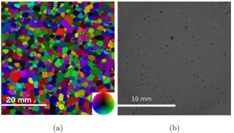
represented on Figure 1a. One can observe that there is no preferred c-axis 125
orientation in the specimen and grains are equiaxed. 126
In addition, micro-computed tomography has been conducted on one 127
specimen (voxel size of 14 µm in this case) to evaluate the manufacture 128
of the specimen regarding the presence of pores. The result is presented on 129
Figure 1b in which it can be observed that the porosity of the specimen is 130
very low. Quantitative analyses of scans from various regions of the specimen 131
led to a density for pores exceeding 1mm in diameter of about 10−3 mm−3.
132
2.2. Spalling test technique
133
The Hopkinson-bar-based spalling test technique is generally used to in-134
vestigate the dynamic tensile strength of quasi-brittle materials from a few 135
tens of s−1 to about 200 s−1. This experimental set-up is made of a short
136
projectile and a slender Hopkinson bar at the end of which the contact with 137
the specimen is made. All the parts are cylindrical with approximately the 138
same diameter. The test creates a short compressive pulse with the projectile 139
propagating in the slender bar and into the specimen. This pulse is reflected 140
into a tensile pulse at the free-end of the specimen, propagating in the oppo-141
site direction and applying tension (Erzar and Forquin [14, 18, 19], Klepaczko 142
and Brara [13], Schuler et al. [20]). This test is well suited for materials that 143
have a higher compressive strength than tensile strength which is the case for 144
polycrystalline ice, according to the literature, at least for quasi-static load-145
(a) (b)
Figure 1: (a) C-axis orientation colour-coded microstructure (see colour-wheel on the bottom right) of specimen #LP06. (b) Slice view of an X-ray micro-tomography of a specimen obtained with the protocol defined in section 2.1. The darkest grey level refers to voids. The scanned area corresponds to the centre of a cross-section of the specimen located at its mid-height. The voxel size is 14 µm3
.
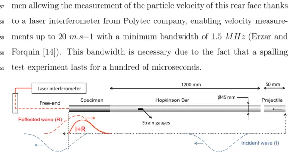
ing rates. The set-up used for these experiments is described in Figure 2. 146
The projectile and the Hopkinson bar are made of high-strength aluminum 147
(7xxx series, yield strength > 450 M P a), which has a 1D wave speed C 148
of 5078 m.s−1, a density of 2800 kg.m−3 and a Youngs modulus equal to
149
72.2 GP a. The diameter of the two components is 45 mm and the bar is 150
1200 mm long. The projectile is 50 mm long and has a spherical-cap-ended 151
nose (radius of 1.69 m) to act as a pulse shaper in order to smooth the load-152
ing pulse Readers are invited to consult (Erzar and Forquin [14]) in which 153
this technique is fully investigated. The Hopkinson bar is instrumented with 154
a strain gauge to measure the compressive pulse applied to the specimen. A 155
reflective paper is fixed (thanks to frozen water) at the free-end of the speci-156
men allowing the measurement of the particle velocity of this rear face thanks 157
to a laser interferometer from Polytec company, enabling velocity measure-158
ments up to 20 m.s−1 with a minimum bandwidth of 1.5 MHz (Erzar and 159
Forquin [14]). This bandwidth is necessary due to the fact that a spalling 160
test experiment lasts for a hundred of microseconds. 161
Incident wave (I)
Reflected wave (R) I+R Free-end 50 mm 1200 mm Laser interferometer Ø45 mm Strain gauges Projectile Hopkinson Bar Specimen
Figure 2: Scheme of the spalling test set-up used in the experiments.
The temperature of the test is an important point. The first idea would 162
be to use a cooled box to assess an accurate temperature around the specimen 163
just before the test. This solution is not suitable here: the only measurement 164
instrumentation on the specimen being the reflective paper at its free-end, 165
the used of an ultra-high-speed (UHS) camera is essential. Then, using a 166
cooling box would prevent capturing good quality images during the test 167
and measuring the particle velocity of the rear face of the specimen with 168
the laser interferometer. A compromise has been made. The specimens are 169
stored in a deep-freezer near their final position in the experimental set-170
up. A protocol has been established in order to ensure that less than 30 171
seconds elapse between the time when the specimen is taken out from the 172
deep-freezer and the time when it is loaded by the spalling test apparatus. 173
This duration has been determined experimentally by doing some trials. A 174
numerical simulation (using a finite-element software) confirmed that no no-175
ticeable warming occurs inside the specimen during 30 s. In particular, the 176
simulated temperature remains constant in the spalled region. A thin frost 177
layer can be observed at the surface of the specimen when taking it out from 178
the freezer but it does not seem to have an influence on the test. 179
During the specimen preparation in the cold room, a cylinder made of 180
the same aluminium alloy as the input bar is glued by mean of frozen water 181
on the specimen. Then, the assembly is put into a deep-freezer set to −30◦C
182
at least the night before the tests. This cylinder is 45 mm in diameter and 183
three lengths were used, 10 mm, 30 mm and 40 mm. Its main roles are (i) 184
to avoid a thermal shock between the ice specimen and the Hopkinson bar 185
which is at room temperature; (ii) to delay the melting of the specimen on its 186
bar side face, which would lead to an impedance discontinuity between the 187
bar and the specimen by the creation of a thin film of water, preventing the 188
load from being correctly transmitted ; (iii) and finally, the position set-up of 189
the specimen, in contact with the input bar, is facilitated. First because an 190
aluminium/aluminium contact has to be set instead of a ice/aluminium one. 191
Second because we designed, on this aluminum cylinder, a holding system 192
made of three pins equally spaced that are connected to pins on the bar 193
by means of springs. This method ensures the best contact between the 194
aluminium cylinder fixed on the specimen, and the bar. The forces applied 195
by the springs are very low and the stress wave propagation is only influenced 196
on its way back, in tension. At this time, the specimen is already broken. 197
3. Test processing 198
3.1. Measurement of the tensile strength
199
Classically, the spalling test technique allows identifying the tensile strength 200
of a material if the assumption of an elastic macroscopic behaviour with no 201
damage of the material before the stress peak is valid (Erzar and Forquin 202
[14], Schuler et al. [20]). In that case, the tensile strength corresponds to the 203
spalling stress leading to the first crack in the specimen and is identified by 204
using the Novikov’s formula as expressed in equation 1 (Novikov et al. [21]). 205
σspall =
1
2ρspecimenCspecimen∆Vpb (1)
where ∆Vpb is the pullback velocity corresponding to the difference
be-206
tween the maximum velocity and the velocity at rebound that are measured 207
on the rear face of the specimen, σspallis the spalling stress leading to fracture
208
(MPa), ρspecimen is the specimen density (kg.m−3) and Cspecimen is the elastic
209
wave speed in uniaxial stress state given by Cspecimen =pEspecimen/ρspecimen
210
where Especimen refers to the elastic modulus of the material specimen. By
211
using this formula, an implicit assumption is made: the celerity of waves in 212
the polycrystalline ice is the same for compressive and tensile waves. The 213
velocity rebound indicates a tensile damage occurring in the specimen dur-214
ing the test. A schematic way to measure it is described in Figure 3. The 215
descending part of the velocity profile corresponds to the tensile phase of the 216
test. 217
Due to the assumptions made in order to establish equation 1 and due 218
to experimental difficulties, several indicators were defined and measured for 219
each test in order to declare it valid or not. These indicators are the wave 220
Rear-face particle velocity
time V
Figure 3: Velocity rebound measurement.
speed in the specimen, the transmitted stress ratio σT/σI in the specimen,
221
σT and σI respectively standing for the transmitted and the incident stresses
222
and the qualitative observation of the crack pattern in the specimen during 223
the test based on high speed photography. Each point is described in the 224
following sections. 225
3.2. Measurement of the wave speed in the specimen
226
Equation 1 allows obtaining the tensile strength of the specimen. Two 227
features of this equation are linked to material properties of the specimen. 228
In the present case, the density of the specimen is quite well known and mea-229
sured during the specimen preparation. Regarding the wave speed C, one can 230
consider it as constant. As explained in equation 1, it depends on the density 231
as well as E which refers to the elastic modulus in one-dimensional uniax-232
ial stress-state. In the present case, the specimen is made of homogeneous 233
ice aggregates which are composed of randomly oriented grains, resulting in 234
an elastic isotropic behaviour (Schulson and Duval [1]). For this case, at 235
−16 ◦C, according to Gammon et al. [16], E
ice = 9.33 GP a. This value was
obtained by exploiting the propagation of sound waves in ice, allowing ob-237
taining a so-called dynamic elastic modulus. In the current study, this result 238
is considered as a reference and, due to this assumption, here, no influence 239
of strain-rate was studied for this parameter. 240
But it is also possible to determine the wave speed from the experiments 241
by using the strain gauge and the interferometer signal. Both are an image of 242
the applied loading, respectively in the bar and in the specimen (one can refer 243
to equations 5 and 6). The idea is to determine the travel time between the 244
strain gauge and the free end of the specimen in order to determine the wave 245
speed. To do so, it is necessary to render the two signals dimensionless and 246
both positive. Then, a cross-correlation analysis is made on the rising stage 247
of the signal. From this analysis, one can obtain ∆t which represents the 248
time delay between the two signals. Then the wave speed in the specimen, 249
Cspecimen, is obtained by equation 2:
250
Cspecimen =
lspecimen
∆t −lgauge to bar end
Cbar
(2) where lspecimen is the specimen length, lgauge to bar end is the length from
251
the gauge to bar-specimen interface, including the intermediate aluminium 252
alloy and Cbar is the wave speed in the bar.
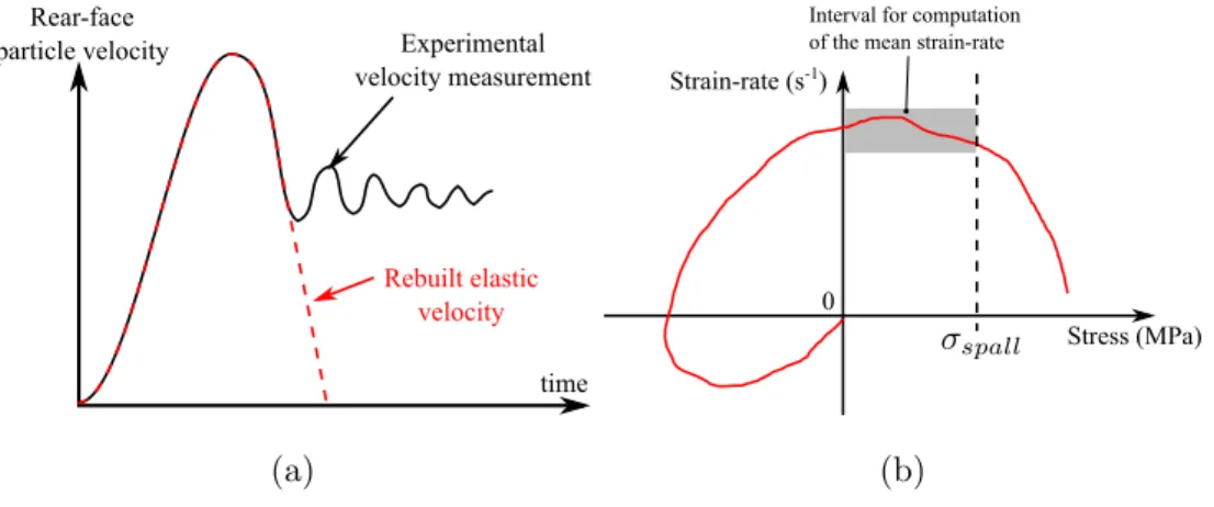
253
Besides the fact that Cspecimen is used to compute the spalling stress
254
(equation 1), this measurement can also be a good indicator of the quality of 255
the contact between the specimen and the bar during the test by checking if 256
its value is reasonable in comparison with an a priori standard value of ice 257
of : 258
Cice = s Eice ρice,(T =−30 ◦C) = s 9.33 GP a 921.6 kg.m−3 = 3182 m/s (3)
where ρice,(T =−30 ◦C) is the corrected density of ice according the expres-259
sion for the temperature dependence of the density of ice (Gammon et al. 260
[16]). 261
3.3. Bar to specimen transmitted stress ratio
262
The impedance of the bar section and of the specimen section can be 263
expressed as Z = SρC with S the cross-section, ρ the density of the material, 264
C its one-dimensional wave speed. Improving the impedance match between 265
the bar and the specimen allows obtaining stress levels high enough in the 266
specimen to damage it during a test, while maintaining the Hopkinson bar 267
and the projectile in their elastic domain. According to the elastic wave 268
propagation theory in the case of a change of impedance section and assuming 269
that the contact is perfect between the bar and the specimen, the ratio α 270
between the incident stress σI coming from the bar and the transmitted stress
271
σT created in the specimen can be expressed as in equation 4:
272 α = σT σI = Z 2 bar Zspecimen + 1 (4) where Zbar = SbarρbarCbar and Zspecimen = SspecimenρspecimenCspecimen.
273
Then α can be used as a quality indicator for the spalling tests performed 274
in this study. The impedance Zspecimen can be computed for each test leading
275
to a theoretical value α0 which can be compared to αexp, the ratio value
276
obtained by measuring σI and σT in a time interval containing the stress
277
peak in compression. 278
The bar remaining in the elastic domain, the measurement of the strain 279
ǫgauge at the gauge location in the bar and the knowledge of the bar’s Young
280
modulus allow measuring σI. σT is obtained by the particle velocity
mea-281
surement V (t) prior to the velocity rebound. Equations 5 and 6 are used: 282
σI(t) = Ebarǫgauge(t) (5)
σT(t) =
1
2ρspecimenCspecimenV (t) (6)
αexp is determined in the compression phase. The evaluation of the test
283
is done by calculating the ratio αexp/α0 . A value around 1 means that the
284
contact between the bar and the specimen is close to being perfect and the 285
closer to 0 the ratio, the lower the quality of contact. If the contact is not 286
good, it does not necessarily mean that the test should not be considered. 287
The input stress is not completely transmitted but the specimen is still un-288
dergoing compression and tension. Often, in this case, the particle velocity 289
from the rear face of the specimen is too far from the expected shape ide-290
alised in Figure 3, making impossible to use equation 1, and so the tensile 291
strength cannot be deduced. 292
3.4. Qualitative test checking with an Ultra High Speed camera
293
An important point of the spalling test experiment is that the specimen 294
has to remain undamaged during the compressive loading phase. This is 295
usually reachable due to the strong compressive strength compared to the 296
dynamic tensile strength of quasi-brittle materials tested with this appara-297
tus. In the present case, the projectile impact velocity needs to be carefully 298
estimated, in order to get strain-rate in the expected range and to ensure 299
that the compressive stress applied to the specimen does not exceed the 300
compressive strength value given by the literature, otherwise the assumption 301
made to use the particle velocity is not valid, making the measurement of 302
the tensile strength impossible. The review done by Schulson and Duval [1] 303
reported a compressive strength around 10 M P a at 10 s−1 for specimens
304
made of fresh-water granular ice in unconfined configuration. Simple elastic 305
numerical simulations of the test were conducted. The aim was to determine 306
the initial projectile velocity to be considered in order to prevent failure due 307
to a compression loading during the test. Then, during the experimental 308
campaigns, the experiments are conducted at different impact velocities to 309
apply different strain-rates. 310
To check if no damage or failure occured during the compression stage, 311
we used an UHS camera (Kirana model from Specialised Imaging). For each 312
test, 180 images with an inter-frame time of 1µs are obtained to visualise 313
the compressive and tensile stages. Due to the transparent properties of ice, 314
one can observe qualitatively the cracks appearing and propagating in the 315
specimen. A test was considered successful if no compression fracture was 316
visible near the contact after analysis of the sequence of images captured with 317
the UHS camera. This point can be very challenging due to the fact that 318
UHS cameras offer a very limited number of pixels in comparison with low 319
speed and reflex cameras. Here, the Kirana model is equipped with one of 320
the biggest sensor regarding the number of pixels (at the time of the study) 321
with 924-by-768 pixels. 322
Figure 4 presents two different cases. On Figure 4a, no crack is visible in 323
the first compressive stage of the test. T0stands for the first picture captured
324
by the UHS camera, a few µs before the compressive pulse reaches the spec-325
imen. Time T0+ 40µs corresponds approximately to the time at which the
326
maximum compressive stress spreads the specimen in the contact zone. At 327
time of T0+80µs, which is fully within the tension stage, fractures are visible
328
and can be linked to the applied tensile loading to the specimen. Conversely, 329
on Figure 4b,a fracture prematurely occurs during the compression at a time 330
of T0 + 40µs. Then, at a time of T0 + 80µs, fractures due to tension are
331
visible. 332
(a) Test visually sucessful. (b) Failed test.
Figure 4: Examples of two series of images obtained from two spalled specimens. (a) No crack in compression is visible, the fracture occurs in tension (test on specimen #LP 20. (b) A premature fracture in compression appears (T0+ 40 µs) then fracture in tension
3.5. Determining the applied strain-rate during tensile stage
333
The last measure to be extracted from the spalling test is the applied 334
strain-rate during the tension stage prior to the tensile damage. The identi-335
fication method used to measure it is based on elastic numerical simulations. 336
For each test, the velocity profile is artificially converted into an elastic pro-337
file. This is achieved by using the rear-face velocity measurement up to the 338
rebound due to spalling. After this point, this curve is virtually prolongated 339
keeping the slope of the tensile phase before spalling fracture. An example is 340
given in Figure 5a. This velocity is converted into a stress using equation 7 : 341
σT(t − ∆t) =
1
2ρspecimenCspecimenV (t) (7)
In this formula V (t) is the velocity history measured by the laser in-342
terferometer, ∆T the traveling time of the wave through the specimen and 343
σT(t − ∆t) the stress which is supposed to be applied at the bar side of the
344
specimen. This stress is used as a loading pulse in the numerical simulation. 345
The exact density and dimensions of each specimen was used for each com-346
putation. Figure 5b shows the type of curve obtained from the simulation 347
to evaluate the strain-rate. For each test, the values are extracted from the 348
results of the numerical simulation at the approximate location of the first 349
appearance of cracks, thanks to the image sequence filmed during the test. 350
The curve is valid up to the spall strength identified with equation 1. To get 351
the minimum, maximum and mean value of the strain-rate, we considered 352
the stress interval beginning with the tensile phase (σ > 0) and ending with 353
σspall. This interval is highlighted in grey in Figure 5b.
Rear-face particle velocity time Experimental velocity measurement Rebuilt elastic velocity (a) Strain-rate (s-1) Stress (MPa) 0
Interval for computation of the mean strain-rate
(b)
Figure 5: (a) Rebuilt of the rear-face velocity to reproduce an virtual elastic loading in numerical simulations. (b) Interval of data taken into account to compute the mean strain-rate of a test.
4. Results and discussion 355
4.1. Validity of the results
356
The main results are presented in Table 2. 357
Tests #LP03, #LP07 and #LP09 were eliminated from this table due 358
to the fact that premature fractures in the compression stage occurred. By 359
looking at the wave speed values, it can be noticed that tests #LP12, #LP13 360
have very low values of one-dimensional wave speed in comparison with the 361
reference value of Cice = 3182m/s and should not be considered. For this
362
reason, the corresponding data are highlighted in dark grey in the table. 363
Regarding αexp values, 7 tests have values quite low in comparison with the
364
theoretical one α0 (#LP01, #LP02, #LP04, #LP05, #LP06, #LP10 and
365
#LP11), which means that the quality of the contact during these tests is 366
really poor. Those results are highlighted in light grey in Table 2. Conversely, 367
for the other tests, the αexp/α0ratio is around 1, representing a good contact.
Table 2: Summary of the obtained results (dark grey: very low values of one-dimensional wave speed, light grey: low values of alpha, italic: result to be confirmed by further investigations.) Spec Id # Cspec (m/s) αexp (%) αexp/α0 (%/%) σspall (M P a) ˙ǫmean (s−1) ˙ǫmin− ˙ǫmax (s−1) LP01 3236 22,9 0,67 4,9 71 59-75 LP02 3389 16,7 0,47 3,1 34 24-37 LP04 2830 24,5 0,8 3,8 109 102-113 LP05 3189 19,6 0,58 3,4 49 36-53 LP06 2970 25,5 0,8 4,7 103 96-108 LP08 3499 42,7 1,16 16,3 271 255-283 LP10 3121 16,2 0,49 2,1 38 33-40 LP11 2978 21,3 0,67 3,3 89 81-93 LP12 2382 14,4 0,54 2,5 81 71-88 LP13 2235 6,3 0,25 1,4 51 47-54 LP14 3040 33,5 1,03 4,3 107 91-116 LP15 2654 27,3 0,93 1,9 41 37-44 LP16 2917 33,2 1,05 4,0 121 107-131 LP17 2992 33,1 1,04 4,4 110 99-117 LP18 2962 34,0 1,07 4,1 108 95-115 LP19 2881 33,0 1,07 4,3 120 111-126 LP20 3009 34,5 1,08 3,8 83 74-88 LP21 2793 32,5 1,07 3,2 69 58-76
This fact can be explained by the experimental technique that has been used. 369
Indeed, it was mentioned that two campaigns were conducted for this study. 370
In the first campaign, we set up the specimen on the bar by a simple unilateral 371
contact with no force maintaining this contact. Great care was taken about 372
the position of the specimen and the way to hold it before and during the test 373
and rubber was applied around the intermediate aluminium alloy part and 374
the bar end to prevent some movement. Unfortunately, this way of doing 375
produces very random results on the quality of the contact as it is shown 376
here. Nevertheless, some tests ran well but the setting-up position technique 377
was changed between the two campaigns. In the second one, three springs 378
equally distributed around the bar perimeter applying low-level forces were 379
used to maintain the contact. The quality of the contact, as it can be seen in 380
Table 2 is far more repeatable. Finally, for all the reasons mentioned above, it 381
has been decided to only take into account the results that are not shadowed 382
in Table 2 : only about 50% of the tests were considered as successful. The 383
result obtained with #LP08 has to be confirmed by further investigations. 384
4.2. Tensile strength results
385
On the 9 tests considered here, the strain-rate applied is ranged between 386
41 and 271 s−1. The variation of strain-rate was obtained by having different
387
levels of projectile velocity impact. It can be noticed than the highest value 388
of strain-rate is quite far from the rest of the measured strain-rates. This is 389
due to the fact that only few tests with a high impact velocity of projectile 390
were tried and only one worked out. In the other cases, contact issues or 391
prematurely compressive failure occurred. Finally, the measured spalling 392
stresses, i.e. tensile strengths, range from 1.9 to 16.3 M P a. 393
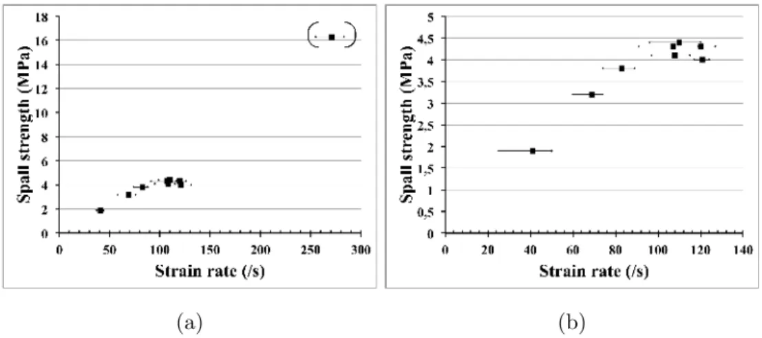
(a) (b)
Figure 6: Tensile strength measurements as a function of strain rate. The shown points indicate the mean values of determined strain-rates. The displayed intervals do not corre-spond to error bars. They correcorre-spond to the minimum and maximum values of strain-rate estimated during the tensile phase.(a) Taking into account #LP08 specimen. (b) Without #LP08 specimen.
Figure 6a summarises these results in one single graph. As it can be seen 394
in this graph, the influence of the strain-rate on the tensile strength is clearly 395
established. In addition, the obtained values are quite consistent with the 396
reference value of 1 M P a in the quasi-static regime. As the highest point 397
should be confirmed in further investigations, a focus on strain-rates up to 398
120 s−1is presented in Figure 6b. The next logical step of this study would
399
be to spread the test configuration over the full range of strain-rates to better 400
establish the dynamic increase of the tensile strength of polycrystalline ice 401
between the quasi-static and the dynamic regime. 402
4.3. Qualitative analysis of the fracture
403
The use of the UHS camera allowed us detecting premature fracture in 404
compression as well as observing the crack propagation in the volume of 405
the specimen during each test. Even if the latter is a qualitative piece of 406
information, it enables to distinguish three main scenarios as a function of 407
strain-rate, depicted in Figure 7.
(a) #LP15 (41 s−1) (b) #LP21 (69 s−1) (c) #LP17 (110 s−1)
Figure 7: Fracture in the specimen for three different strain-rates. The evolution of the number of cracks clearly visible with the UHS camera increases with the strain-rate.
408
Test #LP15 was one of the tests conducted with the lowest value of mean 409
strain-rate. In the four pictures presented in Figure 7a, only one macro crack 410
can be observed. By contrast, at higher strain-rates such as in Figure 7c 411
(test #LP17), several cracks oriented perpendicularly to the specimen axis 412
develop in a small volume delimited by the white dashed-line rectangle at 413
T0 + 66µs. In the next steps of the test, this zone of damage spreads out
414
towards the bar side of the specimen as observed on the last image where 415
the light saturates. The cracks can be attributed to tensile loading. Finally, 416
the higher the loading rate, the higher the number of cracks activated, which 417
is consistent with the behaviour expected for brittle materials (Forquin and 418
Hild [9]). 419
The result obtained on #LP21 is also interesting. Four images of this 420
test are given in Figure 7b. The mean strain-rate is about 69 s−1. In that
421
case, three distinct cracked zones appear successively during the tensile phase 422
following the propagation of the reflected tensile wave. The rate of the applied 423
strain-rate being lower than in test #LP17, less cracks have been triggered. 424
5. Conclusions 425
This paper presents a first study to evaluate the tensile strength of poly-426
crystalline ice subjected to strain-rates ranging from 41 to 271 s−1. This
427
was achieved by adapting the spalling test technique to polycrystalline ice. 428
The experimental procedure is carefully presented and three indicators are 429
proposed to validate each test: a qualitative optical analysis with an ultra-430
high-speed camera, a quantitative measurement of the wave speed in the 431
material and a quantitative analysis of the quality of the contact with the α 432
ratio (transmitted stress over incident stress). 21 specimens were prepared 433
and 9 tests were considered to present the final results based on the Novikov 434
approximation. The results show that tensile strength is clearly influenced 435
by the strain-rate: at strain-rates around 30 s−1 the tensile strength is found
436
to be about 2 MPa, which is twice the quasi-static value reported in the liter-437
ature (Schulson [7], Petrovic [8]). For strain-rates around 100 s−1, the tensile
438
strength is found to be around 4 MPa. The analysis of the fracture patterns 439
occurring in the specimen during the test confirms also the elastic brittle 440
behaviour of polycrystalline ice in tension of ice in this range of strain-rates. 441
Acknowledgements 442
The present work was developed in the framework of the Brittle’s Codex 443
chair (Fondation UGA) and thanks to the support from the CEA-CESTA 444
(France) and from the Labex OSUG@2020 (ANR 10 LABEX 56). The pro-445
vided support and fundings are gratefully acknowledged by the authors. 446
References 447
[1] E. Schulson, P. Duval, Creep and fracture of ice, Cambridge University 448
Press, doi:https://doi.org/10.1017/CBO9780511581397, 2009. 449
[2] M. Lange, T. Ahrens, The dynamic tensile strength of ice and ice-silicate 450
mixtures, Journal of Geophysical Research 88 (B2) (1983) 1197–1208, 451
doi:https://doi.org/10.1029/JB088iB02p01197. 452
[3] A. Combescure, Y. Chuze-Marmot, J. Fabis, Experimental 453
study of high-velocity impact and fracture of ice, Interna-454
tional Journal of Solid and Structures 48 (2011) 2779–2790, doi: 455
https://doi.org/10.1016/j.ijsolstr.2011.05.028. 456
[4] M. Shazly, V. Prakash, B. Lerch, High strain-rate behavior of ice under 457
uniaxial compression, International Journal of Solid and Structures 46 458
(2009) 1499–1515, doi:https://doi.org/10.1016/j.ijsolstr.2008.11.020. 459
[5] H. Kim, J. Keune, Compressive strength of ice at imact strain 460
rates, Journal of Materials Science 42 (2007) 2802–2806, doi: 461
https://doi.org/10.1007/s10853-006-1376-x. 462
[6] J. Pernas-S´anchez, J. Artero-Guerrero, D. Varas, J. L´opez-Puente, Anal-463
ysis of ice impact process at high velocity, Experimental Mechanics 55 464
(2015) 1669–1679, doi:https://doi.org/10.1007/s11340-015-0067-4. 465
[7] E. Schulson, Brittle failure of ice, Engineering Fracture Mechanics 68 466
(2001) 1839–1887, doi:https://doi.org/10.1016/S0013-7944(01)00037-6. 467
[8] J. Petrovic, Review of mechanical properties of ice and 468
snow, Journal of Materials Science 38 (2003) 1–6, doi: 469
https://doi.org/10.1023/A:1021134128038. 470
[9] P. Forquin, F. Hild, A Probabilistic Damage Model of the Dynamic Frag-471
mentation Process in Brittle Materials, Advances in Aplied Mechanics 472
44 (2010) 1–6, doi:https://doi.org/10.1016/S0065-2156(10)44001-6. 473
[10] E. Cadoni, D. Forni, R. Gieleta, L. Kruszka, Tensile and compres-474
sive behaviour of S355 mild steel in a wide range of strain rates, 475
The European Physical Journal Special Topics 227 (2018) 29–43, doi: 476
https://doi.org/10.1140/epjst/e2018-00113-4. 477
[11] D. Saletti, S. Pattofatto, H. Zhao, Measurement of phase trans-478
formation properties under moderate impact tensile loading in 479
a NiTi alloy, Mechanics of Materials 65, ISSN 01676636, doi: 480
https://doi.org/10.1016/j.mechmat.2013.05.017. 481
[12] K. Xia, W. Yao, Dynamic rock tests using split Hopkinson (Kolsky) 482
bar system – A review, Journal of Rock Mechanics and Geotech-483
nical Engineering 7 (1) (2015) 27 – 59, ISSN 1674-7755, doi: 484
https://doi.org/10.1016/j.jrmge.2014.07.008. 485
[13] J. R. Klepaczko, A. Brara, Experimental method for dynamic tensile 486
testing of concrete by spalling, International Journal of Impact Engineer-487
ing ISSN 0734743X, doi:https://doi.org/10.1016/S0734-743X(00)00050-488
6. 489
[14] B. Erzar, P. Forquin, An Experimental Method to Determine the Tensile 490
Strength of Concrete at High Rates of Strain, Experimental Mechanics 491
ISSN 00144851, doi:https://doi.org/10.1007/s11340-009-9284-z. 492
[15] P. Barnes, D. Tabor, J. C. F. Walker, The Friction and Creep 493
of Polycrystalline Ice, Proceedings of the Royal Society A: Math-494
ematical, Physical and Engineering Sciences ISSN 1364-5021, doi: 495
https://doi.org/10.1098/rspa.1971.0132. 496
[16] P. H. Gammon, H. Kiefte, M. J. Clouter, W. W. Denner, 497
Elastic constants of artificial and natural ice samples by Bril-498
louin spectroscopy., Journal of Glaciology ISSN 00221430, doi: 499
https://doi.org/10.1017/S0022143000030355. 500
[17] C. J. Wilson, D. S. Russell-Head, H. M. Sim, The application 501
of an automated fabric analyzer system to the textural evolu-502
tion of folded ice layers in shear zones, Annals of Glaciology doi: 503
https://doi.org/10.3189/172756403781815401. 504
[18] B. Erzar, P. Forquin, Experiments and mesoscopic modelling of dy-505
namic testing of concrete, Mechanics of Materials ISSN 01676636, doi: 506
https://doi.org/10.1016/j.mechmat.2011.05.002. 507
[19] B. Erzar, P. Forquin, Analysis and modelling of the cohesion strength of 508
concrete at high strain-rates, International Journal of Solids and Struc-509
tures ISSN 00207683, doi:https://doi.org/10.1016/j.ijsolstr.2014.01.023. 510
[20] H. Schuler, C. Mayrhofer, K. Thoma, Spall experiments for the measure-511
ment of the tensile strength and fracture energy of concrete at high strain 512
rates, International Journal of Impact Engineering ISSN 0734743X, doi: 513
https://doi.org/10.1016/j.ijimpeng.2005.01.010. 514
[21] S. Novikov, D. I.I., I. A.G., The study of fracture of steel, aluminium 515
and copper under explosive loading, Fizika Metallov i Metallovedenie 21 516
(1966) 608. 517