Evolution over two decades of the tropical clouds in a subsidence area and their relation to large-scale environment

HAL Id: hal-00856000

https://hal.archives-ouvertes.fr/hal-00856000

HAL is a multi-disciplinary open access archive for the deposit and dissemination of sci-entific research documents, whether they are pub-lished or not. The documents may come from teaching and research institutions in France or abroad, or from public or private research centers.

L’archive ouverte pluridisciplinaire HAL, est destinée au dépôt et à la diffusion de documents scientifiques de niveau recherche, publiés ou non, émanant des établissements d’enseignement et de recherche français ou étrangers, des laboratoires publics ou privés.

Evolution over two decades of the tropical clouds in a

subsidence area and their relation to large-scale

environment

Marjolaine Chiriaco, Hélène Chepfer, Mathieu Reverdy, G. Cesana

To cite this version:

Marjolaine Chiriaco, Hélène Chepfer, Mathieu Reverdy, G. Cesana. Evolution over two decades of the tropical clouds in a subsidence area and their relation to large-scale environment. 2012. �hal-00856000�

Evolution over two decades of the tropical clouds in a subsidence area and their

1

relations to large-scale environment

2

3

M. Chiriaco (1)_{, H. Chepfer} (2)_{, M. Reverdy}(3)_{, G. Cesana} (2)

4

(1) : LATMOS/IPSL, Université de Versailles Saint Quentin, France 5

(2) : LMD/IPSL, Université Pierre et Marie Curie, France 6

(3) : LMD/IPSL, Ecole Polytechnique, France 7

8

9

Submitted to Journal of Geophysical Research 10

Contact: Marjolaine Chiriaco, marjolaine.chiriaco@latmos.ipsl.fr 11 LATMOS 12 11 Boulevard d’Alembert 13 78280 Guyancourt 14 France 15 16

2 2 17

Abstract

18

The interannual variability of cloud properties in a tropical subsidence area (South 19

Atlantic Ocean) is examined using 23 years of ISCCP cloud fractions and optical depths, 20

complemented with ISCCP/Meteosat visible reflectance and a four-years comparison with 21

CALIPSO-GOCCP products. The mean seasonal cloud properties are examined in the area, as 22

their interannual evolution. Circulation regimes (characterized with the SST and w500 from

23

NCEP and ERA-Interim) that dominate summer and winter are also examined, and 24

atmospheric situations are classified in five circulation regimes: ascending air masses, and 25

moderate or strong subsidence with warm or cold SSTs. We examine the mean cloud cover, 26

optical depth, and reflectance in each regime and their evolution in time over 23 years. 27

Observational results (mean values and interannual variability) are compared with simulations 28

from the IPSL and CNRM climate models (part of the CMIP5 experiment), using simulators 29

to ensure that differences can be attributed to model defects. 30

It results that regime occurrence strongly depends on the dataset (NCEP or ERA-31

Interim), as do their evolution in time along 23 years. The observed cloud cover is stable in 32

time and weakly regime-dependent, whereas the cloud optical depth and reflectance are 33

clearly regime-dependent. Some cloud properties trends actually do exist only in some 34

particular regimes. Compared to observations, models underestimate cloud cover and 35

overestimate cloud optical depth and reflectance. Climate models poorly reproduce regime 36

occurrence and their evolution in time, as well as variations in cloud properties associated 37

with regime change. It means that errors in the simulation of clouds from climate models are 38

firstly due to errors in the simulation of the dynamic and thermodynamic environmental 39

conditions. 40

1. Introduction

41

Cloud response to anthropogenic forcing remains one of the main uncertainties for 42

model-based estimates of climate prediction evolution [Soden et al. 2006; Webb et al. 2006; 43

Ringer et al. 2006]. In the Tropics, the response of low level tropical clouds (below 440 hPa)

44

to anthropogenic forcing is highly variable from one climate model to another, suggesting that 45

low-level clouds contribute significantly to tropical climate cloud feedback uncertainties 46

[Bony and Dufresne 2005]. Bony et al. [2004] showed that tropical low-clouds have a 47

moderate sensitivity to temperature, but their statistical weight is so important that they could 48

have a large influence on the tropical radiation budget. As a consequence, it is necessary to 49

study low-level clouds in a context of global warming. 50

Tropical low clouds and their relations to dynamic and thermodynamic variables have 51

been widely studied in the past: in the Pacific Ocean [Clement et al. 2009. Klein et al. 1995. 52

Norris 1998; Norris and Klein 2000; Lau and Crane 1995; Kubar et al. 2010], in the Atlantic

53

Ocean [Zhang et al. 2009; Mauger and Norris 2010; Oreopoulos and Davis 1993], and in all 54

tropical oceans [Williams et al. 2003; Yuan et al. 2008; Klein and Hartman 1993; Sandu et al. 55

2010; Rozendal and Rossow 2003; Medeiros and Stevens 2009; Bony et al. 2004]. Only a few 56

papers are dedicated to the interannual variability of low-clouds: Clement et al. [2009] used 57

fifty years of low cloud observations in the Pacific Ocean and showed for example a positive 58

trend of the total cloud fraction at the end of the 90’s, associated with similar trends in the 59

thermodynamical variables; Oreopoulos and Davies [1993] used cloud satellite observations 60

in two tropical oceanic locations to study the effect of temperature variations on the cloud 61

albedo, in particular its monthly variation during five years. 62

The current paper aims at characterizing the interannual variability of south-Atlantic 63

tropical clouds located in the 0°/30°S – 30°W/8°E square (Fig. 1a), under predominance of 64

subsidence air motion. We have chosen a larger region than the “Namibian” square used in 65

4 4 the KH93, RR03 and Zh09 studies (Tab. 1) because this area is a location of maximum stratus 66

(KH93), and the goal of the current study is to examine all types of clouds associated with 67

subsidence conditions. The high precipitation isolines in Fig. 1a show that the region under 68

study is exposed to the ITCZ (Inter-Tropical Convergence Zone) in the northern edge in DJF 69

(December – January – February), but not in JJA (June – July – August). Most of the time, 70

this region is exposed to the descending air masses of the Hadley cell; in JJA its southern 71

edge could be influenced by the subtropical anticyclone [Venegas et al. 1996]. This region 72

contains both opaque stratocumulus clouds along the African coast, and shallow cumulus 73

clouds westwards (Tab. 1, 3rd _{line). Like previous studies (RR03, Zh09 for the Atlantic}

74

Ocean; Klein et al. 1995; Norris 1998; Norris and Klein 2000 for equivalent subsidence 75

locations in the Pacific Ocean), we analyze DJF and JJA independently because those are 76

opposite seasons in terms of ITCZ influence. 77

The first objective of this paper is to analyze (i) the evolution of montlhy mean cloud 78

radiative properties over two decades in a region of subsidence, and (ii) the evolution of the 79

concommittent dynamic and thermodynamic atmospheric properties. We try to determine if 80

there is a robust relationship between these environmental variables (from reanalysis) and the 81

observed cloud radiative properties (seasonal averaging and spatial resolution of 2.5° x 2.5°), 82

and if this relationship is stable over two decades. It would suggest that we could know cloud 83

radiative properties when dynamic and thermodynamic conditions are known. Moreover, our 84

confidence in model-based predictions of future climate, depends on the ability of models to 85

simulate realisticly the current climate. The second objective of this paper is to evaluate the 86

ability of two climate models to reproduce the evolution over two decades of (i) the observed 87

cloud properties, (ii) the concommittent dynamic and thermodynamic atmospheric conditions, 88

and (iii) the relationship between these environmental conditions and cloud radiative 89

properties. 90

Cloud properties are first characterized using satellite observations (Sect. 2). Then, we 91

focus (Sect. 3) on the characterization of dynamical and thermodynamical regimes and their 92

evolution with time. Sect. 4 describes the cloud properties associated with each regime and 93

their interannual variability. In each section, the main results (i.e. interannual trends) are 94

compared with simulations from the IPSL (Institut Pierre Simon Laplace 4, Hourdin et al. 95

2012) and CNRM (Centre National de Recherches Météorologiques, Voldoire et al. 2011) 96

climate models. Discussion and conclusion are drawn in Sect. 5. 97

98

2. Cloud satellite observations

99

2.1. Satellite data 100

Most papers studying tropical clouds (Tab. 1) are based on satellite observations. 101

Many of those use ISCCP (International Satellite Cloud Climatology Project, Rossow et al. 102

1991a and b; 1993; 1996; 2004) Cloud Fraction (CF), e.g: Clement et al. [2009], Klein and 103

Hartman [1993], Rozendal and Rossow [2003], Williams et al. [2003], Medeiros and Stevens

104

[2009], Zhang et al. [2009], Lau and Crane [1995], Oreopoulos and Davies [1993]. A few 105

papers study tropical low clouds with A-Train observations that give more detailed 106

information on cloud properties: Sandu et al. [2010] used cloud types and cloud fraction from 107

MODIS (Moderate Resolution Imaging Spectroradiometer), associated with collocated 108

observations of water vapor and precipitation; Mauger and Norris [2010] used both MODIS 109

and CERES (Clouds and the Earth’s Radiant Energy System) to study the influence of 110

previous meteorological conditions on sub-tropical cloud properties; Kubar et al. [2010] used 111

the more complex observations from CALIPSO (Cloud Aerosol Lidar and Infrared 112

Pathfinder) and CloudSat along a tropical cross-section during one year. 113

Here, we use three datasets to characterize clouds: cloud fractions and optical depths 114

from ISCCP D2 products [Rossow et al. 1991 and 1996; Rossow and Schiffer 1991], cloud 115

6 6 fractions from CALIPSO-GOCCP (CALIPSO – GCM Oriented CALIPSO Cloud Product, 116

Chepfer et al. 2010), and visible reflectance from ISCCP/Meteosat DX products [Desormeaux

117

et al. 1993]. 118

119

a) ISCCP cloud fraction and optical depth

120

The ISCCP analyzes satellite radiance measurements to retrieve cloud fraction and 121

optical depth. The same algorithms are applied to several spaceborne instruments, such as 122

GOES (Geostationary Operational Environmental Satellite) instruments and Meteosat, or 123

polar orbiters, in order to get long-term information on clouds at global scale. We used the 124

cloud fraction for low-level clouds (CFlow/ISCCP, cloud top pressure Ptop between ground and

125

680 hPa), mid-level clouds (CFmid/ISCCP, Ptop between 680 hPa and 440 hPa), and high-level

126

clouds (CFhigh/ISCCP, Ptop under 440 hPa) as well as the total cloud fraction CFISCCP (sum of CF

127

at the three pressure levels) and optical depth τ, results of the D2 data. Because cloud fraction 128

retrieval is based on passive remote-sensing measurements, there is no overlap between 129

CFlow/ISCCP, CFmid/ISCCP and CFhigh/ISCCP, hence CFISCCP never exceeds 100%.

130

We analyzed 23 years (1984 to 2006) of monthly-mean data averaged seasonally (in 131

DJF and JJA) and spatially at a horizontal resolution of 2.5° x 2.5°. These observations are 132

averaged over the diurnal cycle, unlike the observations used hereafter. 133

134

b) CALIPSO-GOCCP cloud fraction and vertical profile

135

The CALIPSO satellite, launched in 2006, holds the lidar CALIOP (Cloud-Aerosol 136

Lidar with Orthogonal Polarization), which allows the characterization of the cloud vertical 137

structure. The CALIPSO-GOCCP [Chepfer et al. 2010] was initially designed to evaluate 138

cloudiness in Global Circulation Models. It is derived from CALIPSO Level 1 NASA 139

(National Aeronautics and Space Administration) products [Winker et al. 2009] and contains 140

four types of files, including seasonal cloud fraction maps at three levels of altitude (low-, 141

mid-, and high-level defined consistently with ISCCP). As this retrieval is based on active 142

remote sensing, there can be an overlap between the low-level cloud fraction (CFlow/GOCCP),

143

the mid-level one (CFmid/GOCCP), and the high-level one (CFhigh/GOCCP); and the sum of the

144

three can be larger than 100%. Nevertheless, the total cloud fraction CFGOCCP detects if there

145

is a cloud in the column (it does not correspond to the sum of the low, mid and high cloud 146

fraction) and cannot exceed 100%. We also used vertical profiles of cloud fraction 147

(CFGOCCP3D) at 40 equidistant levels (480m) from the ground to 20 km of altitude.

148

We analyzed four years (2007 to 2010) of CALIPSO-GOCCP seasonal mean (DJF and 149

JJA) cloud fractions. Initially, the CALIPSO-GOCCP cloud detection is done at the full 150

CALIOP Level 1 horizontal resolution (330 m along track and 75 m across track) to allow the 151

detection of small-size fractionated boundary layer clouds; cloud occurrences are then 152

statistically summarized over 2.5° x 2.5° grid box consistently with ISCCP cloud fraction. 153

The CALIPSO-GOCCP cloud fraction reported here are collected in day-time (1330 LST, A-154

train orbit). In the current study, this product helps to understand the vertical distribution of 155

clouds from one season to another, and from one regime to another, but is not used to draw 156

any trend. 157

158

c) ISCCP/ Meteosat visible reflectance

159

To consolidate our analysis, and avoid making it dependent of the inversion 160

algorithms, we also use Meteosat Level 1 reflectance measurements (visible, wavelength near 161

0.6 µm) from ISCCP/Meteosat DX files. Reflectance can be seen as a proxy of cloud fraction 162

combined to cloud optical depth: a radiative signature of the cloud scene. 163

Since we focus on a given geographical zone, the satellite viewing direction is 164

constant; moreover the analysis is not impacted by the change of instruments as shown by 165

8 8 clear sky evolution in Appendix A. We use reflectance observed at a constant time 1200 UTC 166

(3-hours time slot, as close as possible to the CALIPSO overpass time), seasonally averaged 167

(DJF and JJA) during 23 years. The horizontal resolution is 0.5° x 0.5°, and the reflectance 168

uncertainty is 0.004. Since the satellite azimuthal relative angle changes with the season, DJF 169

and JJA reflectance cannot be compared in a quantitative way. Nevertheless, as the angles are 170

the same every year at the same date and same location, the same seasons can be compared 171

over different years, in order to study the interannual variability (Appendix A). Typically, 172

stratus (St) are associated with higher reflectance than stratocumulus (Sc), cumulus (Cu) 173

being the less reflective. 174

175

2.2. Cloud properties observed by satellite in the region under study: main patterns 176

177

a) Spatial distribution

178

Reflectance value is high in three regions (Fig. 1i-j): northeast, southwest and mid-179

east, all with low standard deviations suggesting homogeneity of cloud solar reflectivity over 180

years. This is consistent with previous studies that found a lot of stratus in this area, even if 181

the area of maximum reflectance is not completely contained in the Namibian square studied 182

previously (KH93, RR03, Zh09). 183

The mid-east region is characterized by important cloud fractions (about 0.8) observed 184

by both GOCCP (Fig. 1b-c) and ISCCP (Fig. 1e-f) with low standard deviations (not shown), 185

and large optical thickness (τ ~ 8, Fig. 1g) with important standard deviations (not shown). 186

This suggests that low clouds are present most of the time in this region but their cloud optical 187

thickness is highly variable (probably due to transitions between different types of low 188

clouds). This region corresponds with the “Namibian” area studied in KH93 who show that 189

stratus clouds are more frequent in JJA than in DJF (0.67 versus 0.6): opposite result is found 190

for CFISCCP (Fig. e versus Fig. 1f) probably due to the large amount of clouds at higher levels

191

(Fig. 1d). 192

The southwest region shows large cloud fraction (about 0.8) in ISCCP and GOCCP 193

with smaller values of optical thickness (τ ~ 4, Fig. 1i-j). Examining maps for low-/mid-/high-194

cloud fractions from ISCCP and GOCCP (not shown) indicates that this southwest region is 195

mostly characterized by a mix of mid- and high-clouds. 196

197

b) Mean cloud properties

198

When averaged in time over 23 years and spatially over the entire area under study, 199

cloud covers (Tab. 2) show that ISCCP detects almost only low-clouds (about 40%) whereas 200

GOCCP detects some mid- and high-clouds (up to 20%). In complement, the mean vertical 201

profile (Fig. 1d) shows that high-clouds are often present in this area (CFGOCCP3D ~ 20%),

202

with a maxima around 12 km of altitude, and these high clouds are not optically thin enough 203

to mask the important presence of low clouds. 204

The two seasons exhibit similar cloud covers, but the small seasonal variation (less 205

than 10% difference) is different in ISCCP and CALIPSO-GOCCP. The ISCCP cloud 206

fraction CFISCCP and optical depth τ are slightly higher in DJF than in JJA (Tab. 2). This is

207

still the case when considering each year individually (not shown). The seasonal variation 208

from GOCCP is opposite to ISCCP: the mean cloud cover is slightly higher in JJA than in 209

DJF (Tab. 2, Fig. 1b-c-e-f). The discrepancy between ISCCP and GOCCP occurs only in JJA 210

in which GOCCP observes more clouds than ISCCP at all levels of altitudes. The important 211

result is that the difference between the cloud covers from the two datasets is less than 10% 212

for all levels of altitude: both datasets will be used together for the rest of the interpretation. 213

The detailed cloud vertical distribution (Fig. 1d) changes with season: JJA shows less 214

high clouds and more low clouds (CFGOCCP3D ~ 0.25) than DJF. The low cloud variation can

10 1 0 be due in part to the high cloud masking low clouds in DJF. These seasonal differences in the 216

vertical cloud distribution confirm that the cloud types are different during each season in the 217

area under study, and that the two seasons need to be analyzed independently in the rest of 218

this paper (even when split into regime). 219

The results of climate models simulations obtained by the IPSL and CNRM models in 220

the same region and period are given in Tab. 2. Those results have been obtained with the 221

ISCCP [Webb and Klein 2006], CALIPSO [Chepfer et al. 2008] and reflectance simulators 222

[Konsta et al., under review] included in COSP (CFMIP Observations Satellites Package, 223

Bodas et al. 2011). This way, “Climate Model+Simulator” (CMS) outputs are kept consistent

224

with satellite observations. In this region and on average over 23 years, both CMS 225

underestimate by a factor of two the cloud cover whatever the season (Tab. 2), and 226

overestimate significantly the reflectance (up to + 0.1 in JJA), confirming that 1) climate 227

models do not produce enough clouds in the tropics (particularly at low levels), and 2) when 228

models do create clouds, they are optically too thick. This result is consistent with the “too 229

few, too bright” low-level tropical cloud problem identified in CMIP5 models (i.e. Nam et al. 230

2012). 231

232

2.3. Interannual variability of cloud properties (1984-2006) 233

The interannual variability of cloud fraction CFISCCP, optical depth τ and reflectance

234

ref is large over 23 years (Fig. 2) in both DJF and JJA. The trend of each variable, i.e. the

235

value of the linear regression slope multiplied by the number of years is given in each subtitle 236

in Fig. 2 (it is outlined within a rectangle when it is superior to the value of the standard 237

deviation). In DJF, the cloud optical depth τ and reflectance ref have increased in 23 years, 238

despite almost no change in the cloud cover CFISCCP. In JJA, the cloud optical depth has

239

increased of +1.2 in 23 years and reflectance remains almost stable. Anomalies can be 240

isolated: for example, reflectance is enhanced by +0.3 in DJF 1997 and JJA 1985, there is a 241

strong deficit of ref and τ in DJF 1988. Year 1997 corresponds with an El Niño event: the 242

important anomalies of cloud properties for this year are consistent with Belon et al. [2010] 243

results: in the tropics, the fraction of interannual variability of low-cloud cover that is related 244

to SST variability is driven by El Niño index. 245

This important variability in observations is well reproduced by CNRM model, 246

whereas it is smoother with IPSL model (Fig. 2d-e-f). The two models give very different 247

results: they do not show the same years of maximum and minimum for example. For one 248

single model, DJF and JJA are in phase (increase or decrease the same years, maximum and 249

minimum the same years…) whereas it is not the case in observations. 250

251

3. Characterization of the atmospheric circulation in the region under study

252

At first order, the cloud occurrences and optical depth depend on the atmospheric 253

circulation of the air masses; as a consequence, any change in the atmospheric circulation will 254

affect cloud properties. In order to understand if the observed interannual variability of the 255

cloud properties (and its anomalies) is mainly due to variations of atmospheric circulation or 256

to the change in cloud physical processes we will separate the cloud population in 257

atmospheric circulation regimes, based on the analysis of dynamic and thermodynamic 258

variables: in the following, it will be only called “regime”. 259

260

3.1. Definition of the regimes used in this study. 261

Various dynamic and thermodynamic variables are used in the literature to 262

characterize the atmospheric environment in the Tropics. Bony et al. [2004] showed that 263

clouds, and in particular low clouds, are sensitive to both large-scale circulation and 264

thermodynamic structure of the atmosphere. Klein et al. [1995] also concluded that the low-265

12 1 2 level cloud fraction is better correlated to temperatures 24 to 28 hours previously, than to 266

simultaneous ones, and that this cloud fraction is linked to atmospheric circulation at the 267

interannual scale. The Sea Surface Temperature (SST), the Lower Tropospheric Stability 268

(LTS) and the vertical velocity of air at 500 hPa (w500) are also frequently used to characterize

269

the dynamic and thermodynamic state of the atmosphere. Wi03 showed that the clouds 270

response depends more on changes in both w500 and SST than on changes in SST alone.

271

Medeiros and Stevens [2009] suggested that w500 alone is not good to separate low clouds, but

272

is useful with LTS: w500 identifies subsidence and LTS separates cloud types in these

273

subsidence motions. More generally, several approaches have been followed, using only w500

274

as in Bony et al. [2004], only LTS as in Wyant et al. [2009], or a combination of both as in 275

Medeiros and Stevens [2009]. In this study, we privileged the two w500 variable for the

large-276

scale dynamics, and SST variable for the thermodynamics in the following, the combination 277

of these two variables will be called “environmental variables”. 278

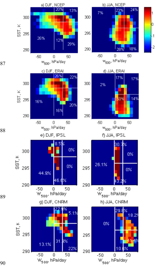
Figures 3 shows the distribution of SSTs and w500 over the region, as simulated by

279

NCEP (National Centers for Environmental Prediction, Fig.3a-b) and ERA-Interim (ECMWF 280

Re-Analyses, Fig 3.c-d) reanalyses, and IPSL (Fig. 3g-h) and CNRM (Fig. 3i-j) climate 281

models. The seasonal variation of SST and w500 is roughly consistent with the position of the

282

Hadley cell in the four models: the SST is colder in JJA than in DJF, and air masses 283

ascending more (w500 < 0) in DJF than JJA. Reanalyses show higher variability than climate

284

models, suggesting than the latter reproduce the mean values for the SST (but not for w500),

285

whereas the real variability is poor for models. In JJA for example, strong subsidence is too 286

frequent and weak subsidence is missing for CNRM model, and strong subsidence never 287

appears for IPSL model. 288

The PDF (Probability Density Function) of w500 and SST from NCEP (not shown)

289

have been examined and values are split following sections of the curves. It leads the 290

separations of the dataset in five regimes (white lines in Fig.3) that are studied independently 291

hereafter: an ascending regime (“As”) associated with deep convection, strong subsidence 292

with cold (“SSu-cold”) or warm (“SSu-warm”) SSTs (associated with Stratocumulus), and 293

weak subsidence with cold (“WSu-cold”) or warm (“WSu-warm”) SSTs associated with 294

trade-wind cumulus). Weak and strong subsidence are separated at 30 hPa/day, and warm and 295

cold SSTs are separated at 298,5 K (respectively 296,5 K) in DJF (respectively JJA). 296

297

3.2. Interannual variability of regime distribution (1984-2010) 298

The occurrence of each regime evolves in time over 27 years (1984 to 2010, in order 299

to get both ISCCP years and GOCCP years). Figure 4 presents the interannual evolution of 300

their occurrence as an anomaly. The interannual trends (calculated as in Sect. 2.3) that are 301

statistically significant (underlined by a rectangle in the subtitle of each subplot in Fig.4), 302

represent about half (11 out of the 20) of the values reported here. A single regime in one 303

season exhibits a consistent interannual trend statistically robust in both datasets (NCEP and 304

ERA-Interim): the occurrence of the As regime decreases by 12-15% in 27 years in DJF. For 305

all other regimes, the trends obtained with the two reanalyses are inconsistent and/or not 306

statistically representative. Moreover, based in NCEP reanalyzes, the As regime is dominant 307

in DJF from 1984 to 1990 whereas SSu-cold dominates 1998 to 2010 (not shown). 308

Similarly to the reanalyses, climate models (Fig. 4f and g) do not suggest a significant 309

change in regime occurrence with time, except for the WSu-warm regime in DJF (only for 310

CNRM model). Nevertheless, this regime becomes more frequent with time in DJF for 311

CNRM model, which is in contradiction with the trend produced by ERA-Interim and NCEP 312

reanalyses. Moreover, trends that are significant in the reanalyses are not significant in the 313

models. 314

14 1 4 This suggests that both climate models are far of reproducing the occurrence of 315

regimes given by the reanalyses, but they are even more far away of reproducing their 316

evolution in time. In particular, the models predict that ascending branch of the Hadley cell 317

(As regime) is more frequent, which is not the case in the reanalyses. 318

319

4. Analysis of cloud properties for each regime

320

4.1. Characterization of cloud properties in regimes 321

To assess how robust is the mean cloud properties dependence on the regime, results 322

obtained with the different satellite datasets (ISCCP, CALIPSO-GOCCP) and reanalyses 323

datasets (NCEP and ERA-Interim) are reported in Fig. 5. 324

Observations (blue and green) are consistent for both datasets: the mean cloud fraction 325

varies slightly (between 0.4 and 0.6) when the regime changes, whereas the mean optical 326

depth (between 3 and 6) and the mean reflectance (between 0.15 and 0.25) are significantly 327

regime dependent, and seasonally dependent. In DJF, the larger optical depth and reflectance 328

are associated with strong subsidence regime (stratocumulus), which optical depth decreases 329

significantly in winter. In JJA, the cloud cover is about the same for all regimes, but larger 330

optical depths (and reflectance) are encountered in deep convection (As regime). These results 331

show that regimes do not drive significantly the mean cloud cover in the region, but do drive 332

the mean cloud optical depth and reflectance, and significantly the vertical structure (Fig. 6). 333

In particular, for the subsidence regime, the SST impacts more the vertical structure than w500,

334

consistently with Wi03 results, in particular in winter (JJA). However, a regime (as defined in 335

this study) does not by itself completely determine the cloud optical depth and reflectance: for 336

a given regime the mean optical depth and reflectance also depend on the season. This 337

seasonal dependency can be explained by the change in the cloud vertical distribution as 338

shown in Fig. 6. 339

Compared to the observations, CMS underestimate the cloud cover (Fig. 5a and d) by 340

a factor of two (or more) in all regimes and seasons, except in the As regime that is better 341

described by one CMS (CNRM). Differences between observations and CMS cloud cover can 342

be more than a factor of three for some regimes: SSu-cold and -warm (but they are not 343

significant in term of population, Fig.3) and WSu-cold in DJF, and SSu-warm in JJA (i.e. 344

41% of the population for CNRM model, Fig. 3h). It confirms that the boundary layer cloud 345

scheme, that drives the amount of cloud forms in subsidence conditions, remains a 346

challenging task for those two climate models. 347

The IPSL model errors on the reflectance (overestimate, Fig. 5c-f) and on the cloud 348

cover (underestimate, Fig. 5a-c) likely compensate to produce correct shortwave fluxes at the 349

top of the atmosphere (in both seasons) as already mentioned in previous section. Figure 5 350

shows that this error compensation applies to all regimes that are significant in term of 351

population. 352

353

4.2. Interannual variability of cloud properties using regime classification 354

Figure 7 shows the trends of observed cloud variables (blue and green bars) over 23 355

years in each regime. It means for example that ref has an increase of +0.03 in 23 years for 356

the As regime in DJF (based on NCEP reanalyses). The cloud fraction is stable in time in all 357

regimes (contrary to Clement et al. 2009), except in the warm strong subsidence regime where 358

it decreases (Fig. 7a) consistently with the reflectance (Fig. 7c). In the other four regimes, 359

cloud optical depth (Fig. 7b) and reflectance (Fig. 7c) have increased very slightly in summer 360

(DJF) over 23 years (about +0.5 for τ and about +0.035 for ref, in 23 years). A more 361

important increase of cloud optical depth occurs in winter (JJA) in all regimes (about +1.5), 362

but it is not associated with change in the reflectance that remains stable in time. 363

16 1 6 A trend is robust if it is observed in both sets of reanalyses, hence the final results are: 364

(1) a decrease of cloud fraction for the SSu-warm regime in DJF, (2) an increase of optical 365

depth for weak subsidence in DJF and for all regimes (except ascent) in JJA, and (3) an 366

increase of reflectance in the ascent regime in DJF. 367

In most of the cases, the IPSL CMS does not show any robust trend in the cloud cover 368

and reflectance. When it shows some trends (vertical arrows in Fig. 7), those are sometimes in 369

contradiction with the observations: in the WSu-warm regime, the modelled CF and ref in 370

JJA increase in time along the last 23 years (Fig. 7c) which is not consistent with the 371

observations. This increase of ref suggests that the clouds of this specific regime reflect more 372

solar light now than 23 years ago. But the observations disagree with this modelled 373 reflectance trend. 374 375 5. Conclusion 376

We have examined cloud properties in a tropical subsidence area (south Atlantic 377

Ocean) using 23 years of ISCCP cloud fractions and optical depths, complemented with 23 378

years of visible reflectance from ISCCP/Meteosat, and cloud vertical profiles from 379

CALIPSO-GOCCP collected during four years. We first studied the mean cloud properties 380

(cloud cover, optical depth, and reflectance) in DJF and JJA. The region under study contains 381

about 40% of low-level clouds and 20% of high-clouds (around 12 km). The difference 382

between ISCCP and GOCCP cloud cover is less than 10%, but the small seasonal variation is 383

not consistent between the two dataset. Then we looked at the interannual variability of cloud 384

properties over 23 years using ISCCP: cloud cover is stable in time and cloud optical depth 385

exhibits a positive trend (+0.55 in DJF and +1.2 in JJA). 386

We compared the observational results with output from climate models (IPSL and 387

CNRM models within CMIP5), coupled with COSP to ensure that differences can be 388

attributed to model defects. Models underestimate cloud cover by a factor of two, and 389

overestimate reflectance (+0.1). The CNRM model produces a stable cloud cover in time, in 390

agreement with observations, whereas the IPSL model shows a significant and unrealistic 391

positive cloud cover trend over the years. 392

As the cloud formation and properties are primarily driven by atmospheric dynamic 393

and thermodynamic variables, we examined the regimes (characterized with the SST and w500

394

from NCEP and ERA-Interim) that dominate DJF and JJA. We classified atmospheric 395

situations in five categories: ascending air masses, moderate subsidence with warm / cold 396

SSTs, strong subsidence with warm / cold SSTs. The occurrence of each regime in the region 397

depends significantly on the dataset used (NCEP or ERA-Interim). The evolution in time of 398

the occurrence of each regime along the 23 years is different and inconsistent in both datasets, 399

except for the “ascending air” regime: its occurrence decreases significantly in time (of more 400

than 10%) according to both datasets. The occurrence of all regimes is poorly reproduced by 401

both climate models (CNRM and IPSL). Moreover, both report an increase in occurrence of 402

the “ascending air” regime contrarily to the observations. 403

We examined the relationship between environmental variables and the observed 404

cloud properties (seasonal averaging and spatial resolution of 2.5° x 2.5°). Observations 405

indicate that the cloud cover (0.4 to 0.6) is slightly regime dependent whereas the optical 406

depth (4 to 6) and the reflectance (0.15 to 0.25) are more significantly regime dependent. 407

Differences between modeled and observed cloud cover and reflectance are not regime 408

dependent. 409

We study the evolution of the relationship between the environmental variables and 410

cloud radiative properties over two decades. The observations exhibit two robust trends over 411

23 years in specific regimes. The optical depth increases only in weak subsidence conditions 412

in DJF (+0.6), and for weak and strong subsidence regimes in JJA (+1). The reflectance 413

18 1 8 increases only for the ascent regime in DJF (+0.03). This later trend is reproduced by IPSL 414

model with a smaller amplitude (+0.01). Trends detected in cloud properties before the 415

regime separation are now explained in some regime, particularly in DJF: the decrease of 416

cloud fraction over 23 years is explained by only one regime (strong subsidence with warm 417

SSTs), as for the optical depth increase which is detected only for weak subsidence, whereas 418

the reflectance increase is not detected in the subsidence (only in ascent). 419

In summary, this study suggests that the main difficulty to built reliable relationships 420

between environmental variables and clouds comes from the significant uncertainties in these 421

environmental variables produced by the different reanalyses and by climate models. It limits 422

the ability to detect robust regime-dependent trend in the observations, and it may be the first-423

order limitation for models to reproduce observed clouds. 424

Future work will consist in extending this study to the entire tropical belt including all 425

CMIP5 models and the same two sets of reanalyses. It will aim at determining if, at this scale, 426

some of the regimes (and related trends) are better reproduced than others and in these cases if 427

the link between cloud properties and environmental variable (and related trends) is better 428

predicted by models. 429

430

Appendix A

432

There are two well-known problems for the retrieval of cloud fraction using satellite 433

passive remote sensing, in particular from the ISCCP program: the variations of the satellite 434

angles, and the calibration of satellites when the instruments are changed. In this Annex we 435

investigate if these problems affect the dataset used in our study. 436

Figure A1.a shows an example of the satellite viewing angle θv for the complete area

437

of study, for one day of the database. The values of this angle are between a few degrees and 438

approximately 40°, depending on the location. Figure A1.b shows the percentage of days 439

when θv is lower or smaller than its median value by more than 2°, for each pixel during the

440

time period of the study. This percentage is always lower than 4%, and Fig. A1.c shows that 441

the concerned θv do not deviate from the median by more than 3°. This shows that, during the

442

23 years of the study, the variations of θv are so small that they should not be a problem for

443

our study of reflectance trends. 444

Figure A2.a is the same as Fig. A1.a but for the satellite relative azimuthal angle φ. 445

The values of this angle are between 0° and 180°, depending on location and time. Figure 446

A2.b is approximately the same as Fig. A1.b but for each pixel, the percentage is calculated 447

every year for the same day, so from 23 values, in order to remove the natural variations of φ 448

and only consider the variations due to technical problems. Another difference is that the 449

percentage is calculated when φ is lower or smaller than its median value by more than 5°. 450

This percentage is about 4% or 8% (one or two cases on twenty three) and Fig. A2.c shows 451

that the concerning φ can be different from the median value by 50°. Figure A3 shows the 452

value of the solar angle for the area under study, in January (Fig. A3a) and in July (Fig. A3b). 453

Using extreme values of these three angles (Fig. A1-A3), the correspondence between 454

reflectance and optical depth values has been calculated. The calculation is done using a 455

doubling/adding radiative transfer code [De Haan et al. 1987], assuming the atmosphere is 456

20 2 0 plane parallel infinite. The atmosphere contains a cloud composed of liquid water spherical 457

particles of 6-µm radius (Mie Theory). Six values of cloud optical depth (τcalc = 0, 1, 5, 10,

458

50, 100) are considered and four different geometries (two extremes of January, and two 459

extremes of July). Figure A4 is an illustration of this calculation (using a linear interpolation), 460

and it shows that for one given optical depth, the reflectance variability is very small from one 461

geometry to another (less than 0.1). 462

Figure A5 shows the variation in time of the clear sky reflectance for the complete 463

time period by selecting, for each day, the smallest reflectance in the area. The figure shows 464

that instrument changes are not associated with any gap in clear sky reflectance values. It 465

follows that instrument changes are not either a problem for the current study that focuses on 466

reflectance. 467

468

Acknowledgments

470

The ISCCP DX data were obtained from the International Satellite Cloud Climatology 471

Project data archives at NOAA/NESDIS/NCDC Satellite Services Group, 472

ncdc.satorder@noaa.gov, on January, 2005. Thanks are also due to the Climserv team for the 473

computing facilities and the data availability. Also thanks to Vincent Noël for internal review. 474

Thanks are due to the reviewers for the very interesting suggestions: it has help for changing 475

and improving the study. 476

22 2 2 References 478 479

Bellon G., G. Gastineau, A. Ribes, and H. Le Treut, 2011: Analysis of the variability 480

of the tropical climate in a two-column framework, Clim. Dyn., DOI

10.1007/s00382-010-0864-481

5 482

Bony S. and J-L Dufresne, 2005: Marine boundary layer clouds at the heart of cloud 483

feedback uncertainties in climate models. Geophys. Res. Lett., 32, No. 20, L20806, doi: 484

10.1029/2005GL023851. 485

Bony S., J.-L. Dufresne, H. L. Treut, J.-J. Morcrette and C. Senior, 2004: On dynamic 486

and thermodynamic components of cloud changes. Clim. Dyn., 22, 71-86. 487

Chepfer H., S. Bony, D. Winker, G. Cesana, J. L. Dufresne, P. Minnis, C. J. 488

Stubenrauch and S. Zeng, 2010: The GCM-Oriented CALIPSO Cloud Product (CALIPSO-489

GOCCP). J. Geophys. Res., 115, D00H16, doi:10.1029/2009JD012251. 490

Clement A. C., R. Burgman, J. R. Norris 2009: Observational and Model Evidence for 491

Positive Low-Level Cloud Feedback. Science, 325(5939), 460-464. 492

Desormeaux, Y., W.B. Rossow, C.L. Brest, and G.G. Campbell, 1993: Normalization 493

and calibration of geostationary satellite radiances for the International Satellite Cloud 494

Climatology Project. J. Atmos. Oceanic Tech., 10, 304-325. 495

Hourdin, F., J.-Y. Grandpeix, C. Rio, S. Bony, A. Jam, F. Cheruy, N. Rochetin, L. 496

Fairhead, A. Idelkadi, I. Musat, J.-L. Dufresne, A. Lahellec, M.-P. Lefebvre, and R. Roehrig, 497

2012 : LMDZ5B: the atmospheric component of the IPSL climate model with revisited 498

parameterizations for clouds and convection, Clim. Dyn., 79, doi:10.1007/s00382-012-1343-y 499

Klein S. A. and D. L. Hartmann 1993: The seasonal cycle of low stratiform clouds. J. 500

Climate. 6(8), 1587-1606.

Klein S. A., D. L. Hartmann, J. R. Norris, 1995: On the Relationships among Low-502

Cloud Structure, Sea-Surface Temperature, and Atmospheric Circulation in the Summertime 503

Northeast Pacific. Journal of Climate, 8(5), 1140-1155. 504

Konsta D., JL. Dufresne, H. Chepfer, A. Idelkali, G. Cesana, 2012: Evaluation of 505

clouds simulated by the LMDZ5 GCM using A-train satellite observations (CALIPSO-506

PARASOL-CERES), Clim. Dyn., under review 507

Kubar T. L., D. E. Waliser, and J.-L. Li, 2010: Boundary layer and cloud structure 508

controls on tropical low cloud cover using A-Train satellite data and ECMWF Analyses. J. 509

Climate, 24, doi: 10.1175/2010JCLI3702.1.

510

Lau N. C. and M. W. Crane 1995: A Satellite View of the Synoptic-Scale 511

Organization of Cloud Properties in Midlatitude and Tropical Circulation Systems. Monthly 512

Weather Review, 123(7), 1984-2006.

513

Mauger G. S. and J. R. Norris 2010: Assessing the Impact of Meteorological History 514

on Subtropical Cloud Fraction. J. Climate, 23(11), 2926-2940. 515

B. Medeiros and B. Stevens, 2009: Revealing differences in GCM representations of 516

low clouds, Clim. Dyn., 36, 385 – 399. 517

Nam C., S. Bony, JL Dufresne, H. Chepfer, 2012: The 'too few, too bright' tropical 518

low-cloud problem in CMIP5 models, Geophys. Res. Lett., idoi:10.1029/2012GL053421. 519

Norris J. R., 1998: Low cloud type over the ocean from surface observations. I. 520

Relationship to surface meteorology and the vertical distribution of temperature and moisture. 521

Journal of Climate, 11(3), 369-382.

522

Norris J. R. and S. A. Klein 2000: Low cloud type over the ocean from surface 523

observations. Part III: Relationship to vertical motion and regional surface synoptic 524

environment. J. Climate, 13(1), 245-256. 525

24 2 4 Oreopoulos L. and R. Davies, 1993: Statistical dependence of albedo and cloud cover 526

on sea surface temperature for two tropical marine stratocumulus regions. J. Climate, 6, 2434-527

2447. 528

Ringer, M.A. et al., 2006. Global mean cloud feedbacks in idealized climate change 529

experiments. Geophys. Res. Lett., 33(7), L07718. 530

Rossow W. B. and R. A. Schiffer, 1991: ISCCP cloud data products. Bull. Amer. 531

Meteor. Soc., 72, 2–20.

532

Rossow W. B., L. C. Garder, P. J. Lu, and A. W. Walker, 1991: International Satellite 533

Cloud Climatology Project (ISCCP), documentation of cloud data. WMO/TD-266 (revised), 534

World Climate Research Programme (ICSU and WMO), Geneva, Switzerland, 76 pp. plus 3 535

appendixes. 536

Rossow W. B., A. W. Walker, and L. C. Garder, 1993: Comparison of ISCCP and 537

other cloud amounts. J. of Climate, 6, 2394–2418. 538

Rossow W. B., D. E. Beuschel, and M. D. Roiter, 1996: International Satellite Cloud 539

Climatology Project (ISCCP) documentation of new cloud datasets. WMO/TD-737, World 540

Climate Research Programme (ICSU and WMO), Geneva, Switzerland, 115 pp. 541

Rossow W.B. and E. Duenas, 2004: The International Satellite Cloud Climatology 542

Project (ISCCP) web site: An online resource for research. Bull. Amer. Meteorol. Soc., 85, 543

167-172. 544

Rozendaal, M.A., and W.B. Rossow, 2003: Characterizing some of the influences of 545

the general circulation on subtropical marine boundary layer clouds. J. Atmos. Sci., 60, 711-546

728. 547

Sandu I., B. Stevens, and R. Pincus, 2010: On the transitions in marine boundary layer 548

cloudiness. Atmospheric Chemistry and Physics, 10(5), 2377-2391. 549

Soden, B.J., and I.M. Held, 2006: An assessment of climate feedbacks in coupled 550

ocean-atmosphere models. Journal of Climate, 19(14), 3354-3360. 551

Venegas S. A., L. A. Mysak, and D. N. Straub, 1996. Evidence for interannual and 552

interdecadal climate variability in the south atlantic. Geophys. Res. Lett., 23(19), 2673-2676. 553

Voldoire A., E. Sanchez-Gomez, D. Salas y Mélia, B. Decharme, C. Cassou, S. 554

Sénési, S. Valcke, I. Beau, A. Alias, M. Chevallier, M. Déqué, J. Deshayes, H. Douville, E. 555

Fernandez, G. Madec, E. Maisonnave, M.-P. Moine, S. Planton, D. Saint-Martin, S. Szopa, S. 556

Tyteca, R. Alkama, S. Belamari, A. Braun, L. Coquart, F. Chauvin,2011: The CNRM-CM5.1 557

global climate model: description and basic evaluation, Clim. Dyn., accepted, 558

DOI:10.1007/s00382-011-1259-y 559

Webb, M.J. et al., 2006: On the contribution of local feedback mechanisms to the 560

range of climate sensitivity in two GCM ensembles. Climate Dynamics, 27, 17-38. 561

Williams K. D., M. A. Ringer, and C. A. Senior, 2003: Evaluating the cloud response 562

to climate change and current climate variability. Climate Dynamics, 20, 705-721. 563

Winker D. M., M. A. Vaughan, A. Omar, Y. X. Hu and K. A. Powell, 2009: Overview 564

of the CALIPSO mission and CALIOP data processing algorithms. J. Atmos. Ocean. Tech. 26 565

2310-2323. 566

Wyant M., C. Bretherton, and P. Blossey, 2009: Subtropical low cloud response to a 567

warmer climate in an superparameterized climate model: Part I. Regime sorting and physical 568

mechanisms. Journal of Advances in Modeling Earth Systems, 0(0). 569

Yuan, J. and D. L. Hartmann, 2008: Spatial and Temporal Dependence of Clouds and 570

their Radiative Impacts on the Large-scale Vertical Velocity Profile. J. Geophys. Res., 571

113(D19201): doi:10.1029/2007JD009722.

572

Zhang Y. Y., B. Stevens, B. Medeiros, M. Ghil, 2009: Low-Cloud Fraction, Lower-573

Tropospheric Stability, and Large-Scale Divergence. J. Climate, 22(18), 4827-4844. 574

26 2 6

List of Tables

575

Table 1: Review of previous studies concerning tropical low clouds and their relations

576

to dynamic and thermodynamic variables, when the area of study includes part of total of the 577

location of the following paper, called A. *SON is for September to November, MAM is for 578

March to May, MJJAS is for May to September, NDJFM is for November to March; **Cloud 579

Top Pressure; ***Sc for Stratocumulus, Cu for Cumulus. 580

Table 2: Mean values (0° - 30°S, 30°W – 8°E) of the entire database for ISCCP (1984

581

– 2006) and CALIPSO-GOCCP (2007 – 2010). Equivalent simulated values from the IPSL 582

and CNRM models have been added when available. 583

584

585

587

Reference Important results in the A area Location

Klein and Hartman 1993

[KH93]

- SON* is season of maximum stratus & maximum LTS - A is an area of maximum stratus

- interannual variability in stratus are related to changes in LTS

Area contained in A Rozendal and Rossow 2003 [RR03]

- CFlow(MJJAS*) > CFlow(NDJFM*)

- notable differences between the low cloud areas in Pacific and the low cloud areas in Atlantic (CF, τ, CTP**…)

- more the subsidence is important, more the cloud top is low

Area contained in A

Sandu et al. 2010

[Sa10] - transition of decrease CF associated with strong increase of SST & decrease of LTS, & free troposphere gradual humidification - Sc to Cu*** transition is stable from one Ocean to another, but Sc CF is higher in South Hemisphere Oceans

All Atlantic Ocean

Williams et al.

2003 [Wi03]

- cloud response depends more on w500 & SST changes than on

SST changes only

- low clouds: many with medium τ, CF more important for strong subsidence and cold SSTs

All tropical oceans

Medeiros and Stevens 2009

[MS09]

- CFlow increase as LTS increase but is independent of w500

- the peak of CFlow is about 30%, very large and very low values

of CFlow are rare

- in A: a few shallow-Cu at high level, a lot of Sc at low level

All tropical oceans

Zhang et al. 2009

[Zh09] - CF- CFlowlow increases linearly as a function of LTS & LTS: both are maximum in SON* and minimum in

MAM* Area contained in A Oreopoulos and Davies 1993 [OD93]

- SST has negative correlation with Albedo and CF, also for

interannual variations Area contained in A

Bony et al. 2004

[Bo04] - low clouds have moderate sensitivity to temperature change but have an important statistical weight, so a large influence on the tropical Radiative budget

- cloud Radiative forcing is high for ascendance and small for subsidence

All tropical oceans

588

Table 1: Review of previous studies concerning tropical low clouds and their relations to

589

dynamic and thermodynamic variables, when the area of study includes part of total of the

590

location of the following paper, called A. *SON is for September to November, MAM is for

591

March to May, MJJAS is for May to September, NDJFM is for November to March; **Cloud

592

Top Pressure; ***Sc for Stratocumulus, Cu for Cumulus.

593

28 2 8 595 CFISCCP DJF JJA τISCCP DJF JJA CFGOCCP DJF JJA ref DJF JJA Low – obs 0.46 0.39 _ _ 0.39 0.47 _ _ Mid – obs 0.05 0.07 _ _ 0.13 0.11 _ _ High – obs 0.01 0.03 _ _ 0.20 0.16 _ _ Tot – obs 0.52 0.49 4.21 3.97 0.52 0.56 0.18 0.15

Tot – mod IPSL 0.18 0.17 _ _ 0.21 0.20 0.2 0.3

Tot – mod CNRM 0.22 0.21 _ _ 0.26 0.26 _ _

596

Table 2: Mean values (0° - 30°S, 30°W – 8°E) of the entire database for ISCCP (1984 – 2006)

597

and CALIPSO-GOCCP (2007 – 2010). Equivalent simulated values from the IPSL and

598

CNRM models have been added when available.

599

600

List of figures

602

Figure 1: Area under study. a) Isolines of NCEP precipitable water for entire

603

atmosphere (1984 – 200WSu-cold6), every 3 kg/m², only larger than 35 kg/m² highlighting 604

ITCZ area. Red is July, blue is January. Dotted square is the area of current study, dashed one 605

is the area of KH93 study; b-c) Mean CFGOCCP (2007 – 2010) (DJF-JJA); d) CFGOCCP3D mean

606

vertical profile (2007 – 2010); e-f) same as b-c) for CFISCCP (1984 – 2006); g-h) for τ; i-j), for

607

ref.

608

Figure 2: Evolution of the mean cloud properties anomaly from 1984 to 2006. a)

609

CFISCCP; b) τ; c) ref; d) CFISCCP from models; e) CFGOCCP from models; e) ref from models.

610

Blue for DJF observed, red for JJA observed, black for JJA IPSL model, brown for JJA 611

CNRM model, magenta for DJF IPSL model, green for DJF CNRM model. Horizontal dashed 612

lines correspond to the values of standard deviations. Numbers in the titles are values of 613

trends in 23 years, and the significant ones (i.e. superior to the variability – standard 614

deviation) are in rectangles. Blue vertical lines indicate particular years in DJF, red ones the 615

same in JJA, and black ones particular years in both DJF and JJA. 616

Figure 3: Log of percentage of occurrence of SST values (by classes of 1 K) versus

617

w500 values (by classes of 10 hPa/day) from 1984 to 2010. a) NCEP in DJF; (b) NCEP in JJA;

618

(c) ERA-Interim in DJF; d) ERA-Interim in JJA; e) IPSL model in DJF; f) IPSL model in 619

JJA; g) CNRM model in DJF; h) CNRM model in JJA. (white horizontal and vertical lines 620

indicate the limits of the five dynamical regimes and the number in white are the percentage 621

of pixels of each regime). 622

Figure 4: a-e. Anomaly of the percentage of pixels of each dynamical regime from

623

1984 to 2010 (DJF in blue, JJA in red) defined by NCEP w500 and SST values. a) As, b)

WSu-624

cold, c) WSu-warm, d) SSu-cold, e) SSu-warm. The horizontal dashed lines correspond to the 625

values of standard deviations. Values of the trends in 27 years are indicated in the titles for 626

30 3 0 both NCEP and ERA-Interim reanalysis, and the significant ones are in rectangles. Vertical 627

lines are the same as in Fig. 2. f-g. Equivalent trends (the value of the linear regression slope 628

of the curve, multiplied by the number of years) values over 27 years for DJF (f.) and JJA (g.) 629

calculated from NCEP, ERA-Interim, IPSL model, CNRM model. Significant trends are 630

indicated by an arrow. 631

Figure 5: Mean values of cloud properties for the five dynamical regimes. Three first

632

lines are CF, τ, and ref in DJF, three last lines the same in JJA. Blue bars are based on NCEP 633

reanalyses, green ones on ERA-Interim reanalyses. Same results from models (IPSL and 634

CNRM) have been added (not colour bars). 635

Figure 6: mean vertical profile of CFGOCCP3D (2007 – 2010). The complete database

636

are represented by the black dotted lines, it is then separated onto the five regimes. a) in DJF; 637

b) in JJA. X axis is in logarithmic scale. 638

Figure 7: Same as Fig. 5 but for trend values (over 23 years) instead of mean values.

639

A “trend” is the value of the linear regression slope of the curve, multiplied by the number of 640

years. CFGOCCP values are not drawn as there are too few years for trend estimation. Black

641

arrows are added when the trend is superior to the variability (i.e. the standard deviation). 642

Same results from models (IPSL and CNRM) have been added (not colour bars). 643

Figure A.1: Satellite viewing angle θv (a) example of values in January, (b) 644

percentage of values that are more than 2° lower or larger than the median value for the entire 645

time period, (c) mean value of the difference between θv and its median when the percentage

646

of (b) is non-zero. 647

Figure A.2: Satellite azimuthal relative angle φ (a) example of values in January, (b)

648

percentage of values that are more than 5° lower or larger than the median value for the entire 649

time period, (c) mean value of the difference between φ and its median when the percentage 650

of (b) is non-zero. 651

Figure A.3: (a) Solar zenithal angle at 1200 UTC on January 15th; (b) same as (a) but 652

on July 15th. 653

Figure A.4: Simulation of the reflectance as a function of the optical thickness, for

654

four representation of the satellite geometry: solar zenithal angle of 20°/angle of viewing 655

direction with nadir of 15°/relative viewing azimuth angle of 50° (characteristic of January, 656

red plane line), 32°/15°/50° (characteristic of January, blue plane line); 22°/42°/130° 657

(characteristic of July, red dashed line); 50°/42°/130° (characteristic of July, red dashed line). 658

Figure A.5: Time evolution of the clear sky reflectance, during the complete period

659

(in blue). Satellite changes are indicated by vertical red lines. 660

661

32 3 2 663 664 665 666 667

Figure 1: Area under study. a) Isolines of NCEP precipitable water for entire atmosphere

668

(1984 – 2006), every 3 kg/m², only larger than 35 kg/m² highlighting ITCZ area. Red is July,

669

blue is January. Dotted square is the area of current study, dashed one is the area of KH93

670

study; b-c) Mean CFGOCCP (2007 – 2010) (DJF-JJA); d) CFGOCCP3D mean vertical profile

671

(2007 – 2010); e-f) same as b-c) for CFISCCP (1984 – 2006); g-h) for τ; i-j), for ref.

672 673 a) b) c) e) f) g) h) i) j)

674

675

676

677

Figure 2: Evolution of the mean cloud properties anomaly from 1984 to 2006. a) CFISCCP; b)

678

τ; c) ref; d) CFISCCP from models; e) CFGOCCP from models; e) ref from models. Blue for DJF

679

observed, red for JJA observed, black for JJA IPSL model, brown for JJA CNRM model,

680

magenta for DJF IPSL model, green for DJF CNRM model. Horizontal dashed lines

681

correspond to the values of standard deviations. Numbers in the titles are values of trends in

682

23 years, and the significant ones (i.e. superior to the variability – standard deviation) are in

683

rectangles. Blue vertical lines indicate particular years in DJF, red ones the same in JJA, and

34 3 4 687 688 689 690

Figure 3: Log of percentage of occurrence of SST values (by classes of 1 K) versus w500

691

values (by classes of 10 hPa/day) from 1984 to 2010. a) NCEP in DJF; (b) NCEP in JJA; (c)

692

ERA-Interim in DJF; d) ERA-Interim in JJA; e) IPSL model in DJF; f) IPSL model in JJA; g)

693

CNRM model in DJF; h) CNRM model in JJA. (white horizontal and vertical lines indicate

694

the limits of the five dynamical regimes and the number in white are the percentage of pixels

695

of each regime).

696 697

698

699

700

Figure 4: a-e. Anomaly of the percentage of pixels of each dynamical regime from 1984 to

701

2010 (DJF in blue, JJA in red) defined by NCEP w500 and SST values. a) As, b) WSu-cold, c)

702

WSu-warm, d) SSu-cold, e) SSu-warm. The horizontal dashed lines correspond to the values

703

of standard deviations. Values of the trends in 27 years are indicated in the titles for both

704

NCEP and ERA-Interim reanalysis, and the significant ones are in rectangles. Vertical lines

705

are the same as in Fig. 2. f-g. Equivalent trends (the value of the linear regression slope of

706

the curve, multiplied by the number of years) values over 27 years for DJF (f.) and JJA (g.)

707

calculated from NCEP, ERA-Interim, IPSL model, CNRM model. Significant trends are

36 3 6 710 711 712

Figure 5: Mean values of cloud properties for the five dynamical regimes. Three first lines

713

are CF, τ, and ref in DJF, three last lines the same in JJA. Blue bars are based on NCEP

714

reanalyses, green ones on ERA-Interim reanalyses. Same results from models (IPSL and

715

CNRM) have been added (not colour bars).

716 717

718

Figure 6: mean vertical profile of CFGOCCP3D (2007 – 2010). The complete database are

719

represented by the black dotted lines, it is then separated onto the five regimes. a) in DJF; b)

720

in JJA. X axis is in logarithmic scale.

721 722 723

38 3 8 724 725 726

Figure 7: Same as Fig. 5 but for trend values (over 23 years) instead of mean values. A

727

“trend” is the value of the linear regression slope of the curve, multiplied by the number of

728

years. CFGOCCP values are not drawn as there are too few years for trend estimation. Black

729

arrows are added when the trend is superior to the variability (i.e. the standard deviation).

730

Same results from models (IPSL and CNRM) have been added (not colour bars).

731 732

733

734

Figure A.1: Satellite viewing angle θv (a) example of values in January, (b) percentage of

735

values that are more than 2° lower or larger than the median value for the entire time period,

736

(c) mean value of the difference between θv and its median when the percentage of (b) is

non-737 zero. 738 739 a b c

40 4 0 740

741

Figure A.2: Satellite azimuthal relative angle φ (a) example of values in January, (b)

742

percentage of values that are more than 5° lower or larger than the median value for the

743

entire time period, (c) mean value of the difference between φ and its median when the

744 percentage of (b) is non-zero. 745 746 a b c

747

Figure A.3: (a) Solar zenithal angle at 1200 UTC on January 15th; (b) same as (a) but on July

748

15th.

749

42 4 2 751

Figure A.4: Simulation of the reflectance as a function of the optical thickness, for four

752

representation of the satellite geometry: solar zenithal angle of 20°/angle of viewing direction

753

with nadir of 15°/relative viewing azimuth angle of 50° (characteristic of January, red plane

754

line), 32°/15°/50° (characteristic of January, blue plane line); 22°/42°/130° (characteristic of

755

July, red dashed line); 50°/42°/130° (characteristic of July, red dashed line).

757

Figure A.5: Time evolution of the clear sky reflectance, during the complete period (in blue).

758

Satellite changes are indicated by vertical red lines.

759 760 761 762 763 764 765