Assessing Multi-rotor UAV Controllability in Low Altitude Fine-Scale Wind Fields

Assessing Multi-rotor UAV Controllability in Low Altitude

Fine-Scale Wind Fields

Alexander H. List and R. John Hansman

This report is based on the Master’s Thesis of Alexander H. List submitted to the Department of Electrical Engineering and Computer Science in partial fulfillment of the requirements for the

degree of Master of Science in Computer Science and Engineering.

Report No. ICAT-2019-12 August 2019

MIT International Center for Air Transportation (ICAT) Department of Aeronautics & Astronautics

Massachusetts Institute of Technology Cambridge, MA 02139 USA

ASSESSING MULTI-ROTOR UAV CONTROLLABILITY IN LOW

ALTITUDE FINE-SCALE WIND FIELDS

by

Alexander H. List and Prof. R. John Hansman

A

BSTRACT

his study presents a means of assessing unmanned aerial vehicle (UAV) control in various environments using control margin. The metric gives an instantaneous measure of control authority and is defined by dividing required torque by maximum available torque. Required torque is the sum total of torque developed by a vehicle's rotors and residual terms representing the torque required to compensate for any remaining disturbances. The metric was demonstrated on a representative small quadrotor UAV in real world and laboratory environments. Utilizing only rotor revolutions per second and inertial measurement unit information, the metric indicates degraded control in conditions consistent with loss of control. This metric may ultimately be useful in understanding the low level wind environment, for certification of vehicles, or for real-time monitoring of control authority.

A

CKNOWLEDGEMENTS

This work was supported by the FAA Joint University Program (DOT/FAA grant 16-G-011). The authors would also like to acknowledge the motivation and technical input of David Sizoo, Wes Ryan, Michelle Yeh and Vicki Ahlstrom.

Contents

2 Defining the Control Margin Metric 21 2.1 Partitioning Control Margin by Axis . . . 21

2.1.1 Angular Velocity Residual . . . 24

2.1.2 Full Form of Metric with Residual . . . 25

3 Experimental Test System 27 3.1 Vehicle Axes for Metric . . . 28

3.2 Instrumentation Payload . . . 28

3.2.1 Payload Mounting and Center of Mass . . . 32

3.3 Data Processing . . . 34

3.3.1 Revolutions Per Second . . . 34

3.3.2 Angular Velocity and Acceleration . . . 35

3.3.3 Filtering . . . 35

3.4 Sum of Torque Calibration . . . 35

3.4.1 Lift Torque by RP S2 _{Calculation . . . . 37}

3.4.2 Inertial Moments . . . 41

3.5 Calculating Max Roll, Pitch and Yaw Torque . . . 45

3.6 Natural Response Time Constant Identification . . . 46

4 Results 49 4.1 Air Jet Impulse Test . . . 50

4.2 Physical Torque Test . . . 52

4.2.1 Physical Torque Test #1 . . . 52

4.2.2 Physical Torque Test #2 . . . 55

4.3 Turbulent Vertical Flow Test . . . 57

4.4 Outdoor Environment Test . . . 60

4.4.1 Outdoor Test #1 . . . 61

4.4.2 Outdoor Test #2 . . . 63

5 Discussion 65 5.1 Limitations and Improvements . . . 66

5.1.1 Infrared Sensors . . . 66

5.1.2 Influences on Max Torque . . . 67

5.1.3 Center of Mass . . . 67

5.1.4 Induced Velocity Model . . . 69

5.1.5 IMU Sampling Rate . . . 70

5.2 Conclusions . . . 70

5.3 Next Steps . . . 71

A Tables 73

List of Figures

1-1 Doubly nested control loops typical of multi-rotor UAVs. . . 19

3-1 The primary axes and rotor spin directions for the Tello quadrotor UAV. 28 3-2 Tello Roll Axis Dynamics. Rotor lift force scaled by distance from the

roll axis (4.32 cm) yields torque. Pitch axis is similar (with a 3.94 cm lever). . . 29 3-3 Tello Yaw Axis Dynamics. Motor torque, depicted, constitutes all yaw

torque for the Tello. . . 29 3-4 The Tello quadrotor UAV with sensor payload. IMU, SD card writer

and IR blade-pass sensor are visible. . . 30 3-5 MicroSD card writer, H048W optical sensors and BNO55 IMU on the

Tello quadrotor UAV. The data log activation switch is also visible. . 30

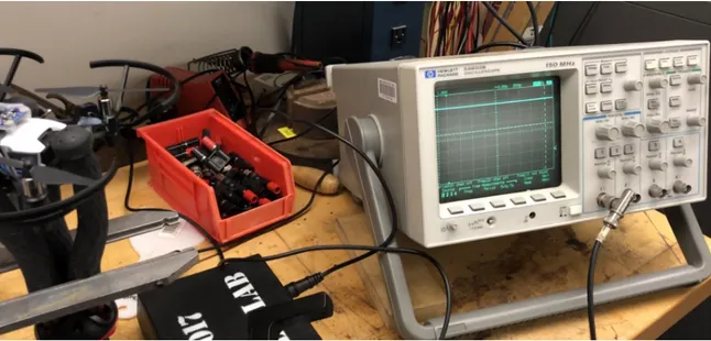
3-6 The Tello on the bench for RPS calibration by an oscilloscope and beam break sensor. . . 31

3-7 Data path and system diagram for the instrumentation payload. . . . 31

3-8 Wiring, Micro JST connectors and hot glue with the instrumentation payload on the Tello quadrotor UAV. The Teensy v3.2 Arduino and battery pack are visible. Nose of the vehicle is at the top of the image,

and the vehicle’s outer-loop optical flow sensors are near the bottom. 32

3-9 Tello COM was measured to be 2 mm forward, 2.4 mm left of the vehicle’s geometric center. . . 33

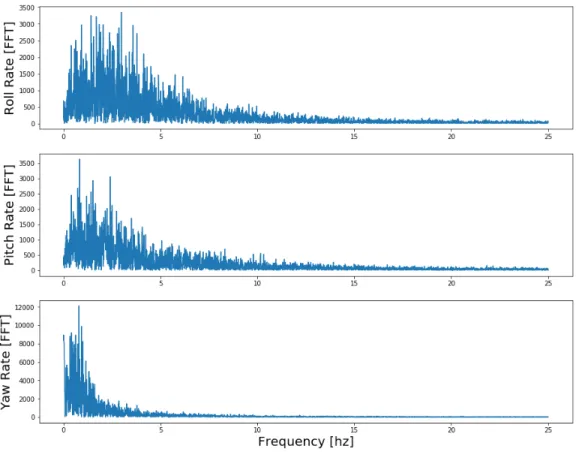
3-11 Gyroscope rates for a Tello flight, absolute value of the Fourier

trans-form. Identified cutoffs: roll and pitch 12.5 hz, yaw 2.5 hz. . . 36

3-12 Effective angle of attack ↵ depends on blade pitch and induced angle . . . 39 3-13 Yaw Torque Match ⌘ Izˆ⇤ ↵yaw/(kmotor⇤P±RP S2). Vehicle torques

itself in still air. There is a minor external interaction with a guide

cord at 1m:29s. Match is not reliable asP±RP S2 _{approaches zero. 44}

3-14 Roll and pitch response period identification during a Physical Torque Impulse Test. . . 47 4-1 Setup of Air Jet Impulse Test. Compressed shop-air jets released into

left tail corner of vehicle (under R0, Fig. 3-1) from a distance of about one foot. . . 50 4-2 Air Jet Impulse Test. Two air impulse jets causing pitch loss of control,

which is indicated for pitch. The first loss of control was deeper than

the second and caused the vehicle to lose more position. . . 51

4-3 Setup of Physical Torque Test #1. Physical pitch-up impulses by tether attached on the nose-side of Tello. . . 53

4-4 Physical Torque Test #1. . . 53

4-5 Setup of Physical Torque Test #2. Physical pitch-up step function by tether attached on the nose-side of Tello. . . 55 4-6 Physical Torque Test #2. Physically pulling-up vehicle pitch from

tail-end of Tello. This example simulates a progressive torquing updraft. Note: a momentary IMU discontinuity at 6m:40s was not removed by filters. . . 56 4-7 Setup of Turbulent Vertical Flow Test. The vehicle is flown over the

vertical-facing shop fan. . . 57 4-8 Turbulent Vertical Flow Test. A high angular velocity yaw loss of

4-9 Setup of Outdoor Environment Test. The vehicle in flight, facing down the corridor and into the wind. . . 61 4-10 Outdoor Test #1. Illustrates roll, pitch and yaw margin degradation

in a low altitude wind field. . . 62 4-11 Outdoor Test #2. A large yaw disturbance and different control margin

change correlations are found in this test. . . 63

List of Tables

3.1 Extremes of inferred center of mass, associated hover torque, and

dis-tance from geometric center, by axis. . . 34

3.2 Tello with Payload Inertial Moments at Geometric Center . . . 42

3.3 Max Torque Values Identified . . . 45

3.4 Natural Time Constant Periods Identified . . . 47

Chapter 1

Introduction

This study concerns itself with the operating limitations of multi-rotor unmanned air vehicles (UAVs) in regard to the low level and fine scale wind environment as may be found in an urban windscape. There is great interest in operating multi-rotor UAVs in low altitude environments for purposes including delivery and urban air mobility [9]. The push towards autonomy and overflight of persons and property makes under-standing the vehicles’ operating limitations important. If control margin, a real-time measure of control authority, is definable, it is possible to measure a vehicle’s sus-ceptibility to various wind environments. Such a technique may ultimately be useful in understanding the low level wind environment, for certification of vehicles, or for real-time monitoring of control authority.

Chapter 1 describes the background research, motivation and objectives for this study. Chapter 2 describes the methods and rationale for developing the control mar-gin metric. Chapter 3 describes the application of the control marmar-gin metric to a small commercially available quadrotor vehicle. Chapter 4 discusses experimental evalua-tion of the control margin metric and results. Chapter 5 discusses the implicaevalua-tions of the research, its limitations and next steps. Appendix A has a table containing nomenclature, and Appendix B compares the control margin metric to a hypothetical time integrated metric.

1.1 Operating Limitations

Traditional airplanes have operating limitations and design requirements in relation to winds. For example, in traditional airplanes, operating limits include crosswind limitations, and design requirements include structural requirements showing integrity under different gust loads.

At this point it is unclear whether the same operating limitations and design requirements should apply to vehicles such as multi-rotor UAVs. One development and certification question is whether multi-rotor UAVs will need to be designed to handle all conceivable winds, or if instead during operations they must land if their control margin is substantially compromised. An objective of this work is to explore this question by developing a metric to measure vehicle controllability in regard to winds.

Adherence to the design requirements of gust loading is often demonstrated through use of system analysis of various wind spectra. Although design criteria such as the Dryden and von Kármán spectrum [7] have been available for analyzing structural loading of flight vehicles in cruise, the low altitude and fine scale environment have not been a focus. The low altitude environment is complicated, for example, by the presence of numerous bluff bodies.

The smaller scale of the vehicles under consideration also means they are suscep-tible to winds finer than have been relevant for vehicles up to this point. The current study defines control margin and shows the feasibility of measuring the response of smaller scale vehicles to various wind environments.

This study presents a means of assessing the controllability of multi-rotor systems. While the ultimate goal for this variety of research would be to characterize the winds in city micro-climates and potentially create a gust spectra specific to the low altitude fine scale wind field, a realistic first goal is to characterize the results of a wind field on particular vehicles. The study of the control margin metric proceeds in this way.

1.2 Controllability

For flight testing of smaller non-transport airplanes, the FAA has described control-lability as the ability to establish, maintain, or alter the attitude of an airplane in regard to its flight path. In particular, the criteria mention that the design of the aircraft should allow “control,” angular displacement, about each of the three main axes: roll, pitch and yaw. In test flights, humans judge the control as “satisfactory” or “unsatisfactory” [3].

A textbook produced for the Navy titled Aerodynamics for Naval Aviators de-scribes “controllability” as the ability of an aircraft to achieve a desired condition of flight adequately, so as to perform takeoff, landing and achieve various maneuvers in flight [4].

Controllability has been defined in Helicopter Controllability [2] as the ability for a vehicle to fly a series of maneuvers required for a mission. In this study, only the ability of a vehicle to maintain its attitude is considered because that is the maneuver required for “the mission” of position control on a multi-rotor UAV.

This study is able to produce a control margin metric with no knowledge of the control system’s desired attitude states, which for most vehicles are roll, pitch and yaw. In this study, the control margin metric is produced with only rotor revolutions per second (RPS) and attitude measurements from an inertial measurement unit (IMU) attached as a payload. Thus the technique described in this study is able to consider an arbitrary vehicle and control system combination without communication with the vehicle.

This study does not define loss of control. However, for the purposes of this study, loss of control is correlated with position loss as well as with attitude loss that remains uncorrected for longer than the vehicle and control system’s natural response period.

1.3 Degraded Modes

All factors related to control of multi-rotor UAVs are aggravated in degraded operating modes such as rotor failures. Multi-rotor vehicles, which maintain flight using the vertical thrust component, usually have rotors placed symmetrically about primary flight axes in order to inherently cancel body torques that would otherwise require asymmetric thrust to maintain stability in normal flight modes. Upon the failure of a single rotor, the thrust generated about (usually all) vehicle axes becomes asymmetric. A good option for vehicles to maintain roll and pitch control in this degraded state is to disable the symmetric rotor for lift maintenance, and utilize it only for attitude control.

The maintenance of yaw in this circumstance depends on the direction of motor spin. Symmetric (co-diagonal) rotors may be spun in the same or opposite directions. Either a rotor spins opposite to its symmetric partner or they rotate in the same direc-tion. In (e.g.) a quadrotor with counter-rotating symmetric rotors, only the roll axis perpendicular to the diagonal shared by the lift-disabled and failed rotor is degraded– in one direction –whereas in a quadrotor with co-directional symmetric rotors, loss of two co-directional rotors means loss of yaw control as well. The quadrotor DJI Tello UAV used as an experimental test system in this study utilizes co-directional symmetric motors, which has the advantage of allowing yaw control without coupling roll and pitch moments, but would lose control of multiple axes in a degraded mode. In any case, the Tello has not been programmed for degraded modes.

With two rotors offline, any multi-rotor UAV has a degraded and potentially lost attitude control in one or more axes, aggravated by a higher percentage utilization on all remaining rotors. In a degraded mode, if more thrust is needed, the vehicle must change its control law to allow error in at least one of yaw, pitch or roll. It is noted that at least one urban air mobility vehicle in development is a quadrotor, which can not be designed to fly with full attitude control in degraded modes. With typical UAV control strategies, symmetric quadrotors only have full attitude control in the no failures case [6]. However, with a model based on this research it would

possible to evaluate the control margin available under the various failure modes of the vehicle, for instance to see which control axes fail first, in order to consider the employment of alternate control strategies and mitigations (e.g. [6, 10]).

1.4 Objectives

This study presents a means of assessing multi-rotor UAV control authority in regard to winds using control margin. The approach defines utilization as the sum of rotor torque output and residual terms representing the torque required to compensate for any remaining disturbances, such as faster-than-control-response winds, divided by the maximum available torque. Control margin is the complement of utilization (cm = 1 |utilization|).

In this study, multi-rotors are UAVs with two or more rotors utilizing the ver-tical component of rotor thrust to maintain flight. This study considers the overall performance of a multi-rotor UAV and its installed control system. While making no assumptions about a particular control scheme, it’s noted that this initial study concerns itself only with a vehicle’s ability to maintain a hover attitude.

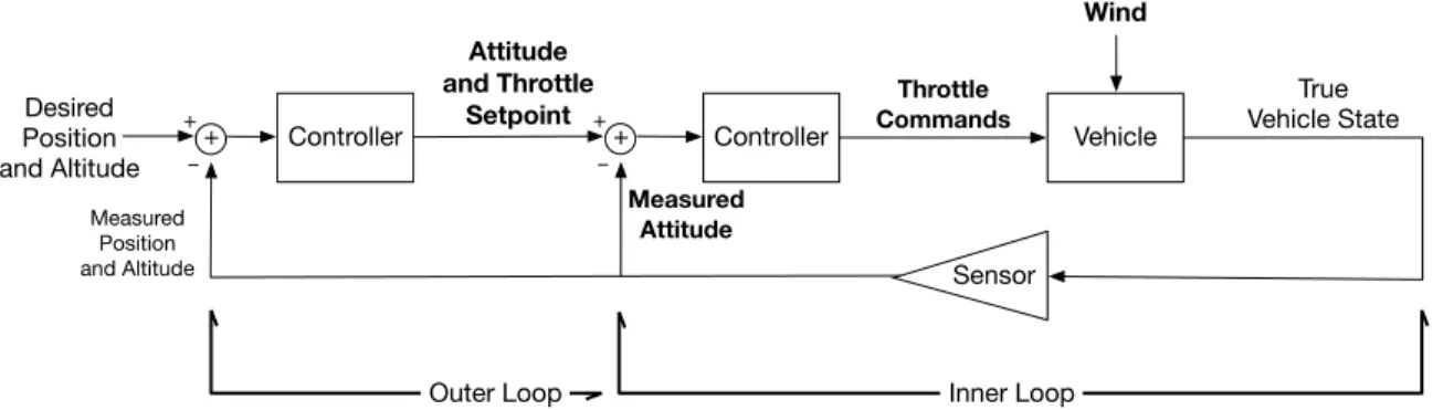
The majority of multi-rotor UAVs are controlled with an outer loop commanding position and an inner loop commanding attitude (Fig. 1-1). In this study, considera-tions are limited to the inner loop, justified by the fact that when the inner loop loses control the outer loop necessarily loses control as well. In fact, outer loop (position) error results from the time integration of inner loop (attitude) error.

_ + + Controller Vehicle Wind True Vehicle State Measured Attitude Throttle Commands Sensor Attitude and Throttle Setpoint Desired Position

and Altitude _ Controller

+ + Measured Position and Altitude Inner Loop Outer Loop

Neither the transient effects of rotor blade inertia change nor gyroscopic precession are considered in this study, nor is a wind shadow effect that can affect multi-rotors in forward flight. A vehicle’s drag profile and rotor downwash on itself is only implicitly considered. Blade flapping which can cause intense vibrations for multi-rotors in longitudinal flight is not included as a disturbance in this initial study.

Further, while some multi-rotor (and single-rotor) UAVs have been demonstrated to maintain inner loop attitude control only by the centrifugal force of a continuously changing attitude, usually yaw [10, 6], only vehicles that have inner loop stability without the need for continuous inertia are considered.

This research does not exhaustively review outer loop loss of control because there are a variety of reasons the outer loop can lose control that do not involve the inner loop, for example, insufficient thrust for the demanded rate of climb. Further, while testing was mostly conducted during vehicle hover, which for multi-rotors can include forward flight, there is no particular restriction on maneuvers that the metric applies to. In fact, there are aspects of the metric’s physics that automatically cancel the torque of angular accelerations for intended attitude changes. For increased accuracy under high angular rate maneuvers, it is possible to utilize desired angular velocity in the metric as well.

The goal of this study is to quantify a metric for “control margin.” The study intended to find a metric that could be used to indicate how close a multi-rotor UAV was to loss of control due to external disturbances, and in particular wind disturbances. The metric is defined as torque required to reject unwanted disturbances divided by torque available.

Chapter 2

Defining the Control Margin Metric

The basic form of the control margin metric is cmˆx = 1 | xˆ|, for a given axis ˆx.

Control margin is the complement of torque utilization, .

Torque utilization metric is an instantaneous metric on the present state of the vehicle, dividing torque required by maximum torque available. Torque required is the sum total of torque developed by a vehicle’s rotors and residual terms representing the torque required to compensate for any remaining disturbances. An acceleration residual expresses unwanted angular acceleration, and a velocity residual expresses unwanted angular velocity by utilizing the natural response time of the vehicle.

2.1 Partitioning Control Margin by Axis

The basic form of the control margin metric is cmxˆ = 1 | xˆ|, where utilization is

the proportion of torque required over the maximum torque the vehicle has available in that axis, Eq. (2.1).

ˆ x =

(⌧xˆ)required

(⌧xˆ)max (2.1)

The control margin metric considers margin on each of the roll, pitch and yaw axes independently. At a high level a multi-rotor vehicle is a 6 degree of freedom device, and the vehicle can directly affect torques about roll, pitch and yaw axes.

The vehicles generally only directly affect position along their vertical axis.

Single axis consideration is a reasonable reduction: Vehicles typically handle roll, pitch and yaw with separate control loops, which combine to allow any desired atti-tude. Regardless of the axis of an external torque, control loss depends on whether any particular axis has lost control.

For an instantaneous controller, a controller where all torque required is instan-taneously provided by the rotors, the torque required in a hover state is defined in Eq. (2.2).

⌧required = rotors_X

(⌧ ) (2.2)

Eq. (2.3) then shows for an instantaneous controller under the single-axis model. =

Protors

⌧

⌧max (2.3)

When maximum torque is provided by this instantaneous controller, = 1 and

cm = 0.

Most vehicles do not have instantaneous controllers. However, the above definition of ⌧required has a grounding in vehicle dynamics for a non-instantaneous controller.

With a strategy of single axis consideration, it’s possible to consider torque utilization due to the dynamics of a single axis at a time, Eq. (2.4).

⌧disturbance+ rotors_X

⌧ = I⇤ ↵measured (2.4)

↵measuredis angular acceleration measured by the IMU. By moving the sum of rotor

torque to the other side of the equation, the torque due to an external disturbance is found as a function of acceleration and rotor torque.

⌧disturbance = I ⇤ ↵measured

rotors_X

⌧ (2.5)

The definition of required torque, now including vehicle body acceleration is Eq. (2.6).

⌧required = ⌧disturbance = rotors_X

(⌧ ) I _{⇤ ↵}measured (2.6)

When the rotors are torquing in one direction, and the vehicle is accelerating in the other, ⌧required becomes larger. This is the behavior desired for torque utilization.

Note that when ↵measured is zero, as in the case of an instantaneous controller,

this equation (2.6) equals Eq. (2.2).

The definition of including ↵measured exists in Eq. (2.7).

= (⌧ )required (⌧ )max = Protors (⌧ ) I_{⇤ ↵}measured ⌧max (2.7)

The body ↵measured acceleration is the motivation for what’s defined as the

resid-ual. The residual can be seen in the general form of the metric, Eq. (2.8). =

Protors

(⌧ ) + Rresidual

⌧max (2.8)

The residual is in units of torque. Residual terms represent the torque required

to compensate for any remaining disturbances after Protors

(⌧ ).

In this study, Rresidual has the terms defined in Eq. (2.9), which are residual terms

for angular acceleration and angular velocity.

Rresidual= R↵+ R! (2.9)

The angular acceleration residual is based on the dynamics equation’s definition of ⌧required and is found in Eq. (2.10).

R↵ = I⇤ ↵measured (2.10)

Up to this point the numerator of , Eq.(2.1), equaled the torque needed to reject the external disturbance torque, ⌧external =Protors(⌧ ) I ⇤ ↵measured.

A conceptual step this thesis takes is that torque required for controllability is not just external torque, but depends also on higher order terms not expressed in the dynamics equation.

Angular acceleration is only the first order residual factor for controllability of a vehicle. A second order factor is angular velocity. Even after an angular accelera-tion is finished, angular velocity (!) remains, which adversely affects controllability depending on its magnitude.

Angular velocity is not directly expressible as torque. Therefore the ! residual is expressed as angular momentum divided by some time constant, Eq. (2.11).

R! =

I⇤ !measured

t (2.11)

2.1.1 Angular Velocity Residual

The time constant chosen for the angular velocity residual is 1/4th _{the vehicle and}

control system’s natural response time for the axis, 1 4tc.

Constant tc is the period in which the vehicle has been demonstrated to cycle

from maximum error to maximum bounce-back for all impulse disturbances within control. The behavior is approximately sinusoidal. If the vehicle can’t stop its inertia at the end of one fourth of this period, it can’t bounce-back by the whole period and has lost control.

The minimum torque required to nullify axis angular momentum in accordance with the natural response time of the vehicle and control system is thus the angular velocity residual, expressed in Eq. (2.12).

The sign is chosen such that a vehicle rotating opposite to the direction of rotor torque has a higher residual.

R! =

I⇤ !measured 1

4tc

(2.12) The explanation for 1/4th _{is the nature of a smooth periodic function and its first}

derivative, namely the 2⇡ periodic sine and cosine. A simple demonstration: suppose sine is angle and cosine angular velocity. Note at ⇡/2 of cosine, the amplitude is zero. Thus, a vehicle must be able to reach zero angular velocity at 1/4th _{the natural}

The time constant enables the conversion of angular velocity to the minimum torque required for complete deceleration within the appropriate period. Other time constants were considered besides natural response time, but alternatives required an arbitrary choice about an attitude limit for considering a vehicle under control.

This study considered vehicles in hover. For off-hover maneuvering conditions, the velocity residual may require an offset by desired !, requiring information from the vehicle control system.

2.1.2 Full Form of Metric with Residual

The full form of the control margin metric is Eq. (2.13). The fraction’s numerator is torque required to maintain control and the denominator is max torque available on the axis. Absolute value is used to keep control margin at or below 1.

cmxˆ = 1 |

Protors

(⌧ ) + Rresidual

⌧max | (2.13)

Substituting the first and second order residuals utilized in this study, Rresidual=

R↵+ R!, the study’s control margin definition is Eq. (2.14). For other applications,

the residual can include higher order torque terms. cmxˆ = 1 |

Protors

(⌧ ) I↵measured I⇤!_0.25measured_⇤tc

⌧max | (2.14)

Chapter 3 describes calculation of sum of torques, max torque, time constants and residuals for a particular test vehicle, and Chapter 4 presents the results of experimental validation.

Chapter 3

Experimental Test System

An experimental test system based on the DJI Tello quadrotor was developed to evaluate the metric. This chapter focuses on calibrating the parameters and obtaining the data required by the control margin metric.

There are two sources of torque on the Tello UAV: the rotors’ lift force acting at a distance to a reference point, and the torque the motors produce to spin the rotors (3.1). The reference point used in this study is the vehicle’s geometric center, and each rotor’s vector from the center of the vehicle is defined ~ri.

rotors_X

~⌧ =

rotors_X

(~ri⇥Lif t~rotor+⌧motor~ ) (3.1)

The control margin metric requires only rotor RPS data and IMU measurements. A description of sensors installed to make these measurements is in § 3.2.

This minimal instrumentation payload allows the calibration of lift and motor torques by RP S2 _{as explained in § 3.4. Max torque is found in § 3.5, and finally the}

natural modes of the vehicle are identified using a physical impulse response method described in § 3.6.

The control system operates relative to the center of the vehicle, but it is invalid to assume that the center of the vehicle is the center of mass, and this is shown in § 3.2.1. The metric reveals the offset center of mass in the hover control margin, which is implicitly accounted for in the calculation of max torque.

3.1 Vehicle Axes for Metric

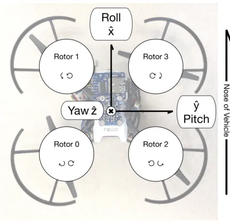
The fundamental flight axes of the vehicle are defined in Fig. 3-1.

Rotor 1 Rotor 0 Rotor 2 Rotor 3

Roll

x̂

ŷ

Pitch

Yaw

ẑ

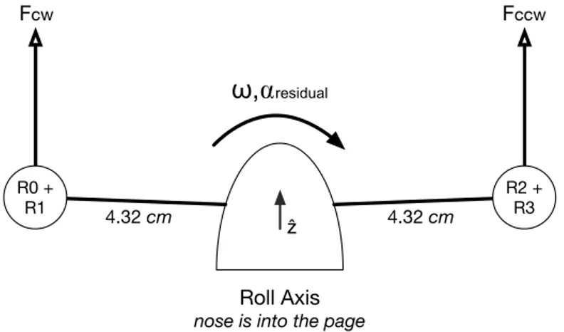
Figure 3-1: The primary axes and rotor spin directions for the Tello quadrotor UAV. As described in § 2.1, each axis of the Tello UAV can be considered separately. Using the rotor numbering in Fig. 3-1, roll torque is the net contribution of torques from rotor0 + rotor1, and rotor2 + rotor3, Fig. 3-2. In the figure, ! and ↵ refer to

the residual disturbances that were not rejected by the control system.

Tello’s yaw torque is the net contribution of motor0+motor3, and motor1+motor2,

Fig. 3-3. Motor torque is the torque with which motors twist the rotor blades. For the Tello quadrotor this constitutes all yaw torque.

3.2 Instrumentation Payload

To measure ! and ↵, the Tello UAV was outfitted with a Adafruit BNO55 Absolute Orientation Sensor. For RPS sensing, H048W Reflective Infrared Optical Sensors

ѡ,⍺residual Fccw Fcw R2 + R3 R0 + R1 ẑ 4.32 cm 4.32 cm Roll Axis

nose is into the page

Figure 3-2: Tello Roll Axis Dynamics. Rotor lift force scaled by distance from the roll axis (4.32 cm) yields torque. Pitch axis is similar (with a 3.94 cm lever).

R0 + R3 R1 + R2 τcw τccw ѡ,⍺residual ẑ Yaw Axis

looking down on vehicle

Figure 3-3: Tello Yaw Axis Dynamics. Motor torque, depicted, constitutes all yaw torque for the Tello.

were installed. Both are connected to a Teensy v3.2 Arduino Board, which writes to a microSD card attached as well (Fig. 3-5).

To measure RPS, reflected IR Sensors detect beam breaks, and the number of blade passes is recorded on the SD card. The presence of a rotor blade is sampled every 120 µs by an interrupt driven C++ program on the Arduino. This was the rate determined to guarantee detection of a rotor blade based on blade width and max RPS (425 RP S). Max RPS was identified using a laboratory beam break sensor attached to a 150 MHz oscilloscope that indicated beam breaks per second (Fig. 3-6). In order to have Tello spin its rotors while on a lab bench, it’s necessary to trick it into believing it is in flight. This is done by lifting the vehicle’s mount during takeoff, ensuring rotor spin-up, then placing it back down. Because the vehicle believes it is

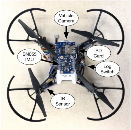
IR Sensor Log Switch SD Card BN055 IMU Vehicle Camera

Figure 3-4: The Tello quadrotor UAV with sensor payload. IMU, SD card writer and IR blade-pass sensor are visible.

Figure 3-5: MicroSD card writer, H048W optical sensors and BNO55 IMU on the Tello quadrotor UAV. The data log activation switch is also visible.

lower than it wants to be, rotors are spun at max RPS at least part of the time. A margin of error was used in the calculation of the appropriate sample rate.

Figure 3-6: The Tello on the bench for RPS calibration by an oscilloscope and beam break sensor.

the session featuring the oscilloscope output were used to ensure the calibration of the IR sensors. Calibration involved adjusting the IR sensor angle, moving IR sensors closer to the rotor blades, and setting voltage thresholds in software. On each rotor, both blades are painted in silver reflective Sharpie ink to increase reflectance (visible in Fig. 3-8).

Attitude data is collected from the payload BNO55 IMU at approximately 50 hz. As soon as IMU data arrives at the Arduino, IMU data and the total number of blade passes are written to the microSD card in csv format. The data flow and separation of instrumentation system concerns is documented in Fig. 3-7.

IR Sensor

H048W Measurement UnitBNO55 Inertial Arduino

120 µs sampling 19.6 ms sampling

On-board SD Card < 20 ms data rate

Blade pass counting Angles and velocities

Tello Quadrotor Pilot Phone Tello Video Footage

3.2.1 Payload Mounting and Center of Mass

The vehicle’s payload would shift between flights, repositioning the vehicle’s center of mass. One center of mass measurement was made after the flight tests, while the center of mass of each flight was inferred by the torque utilized to maintain hover during that flight.

Minor center of mass changes were found to have a substantial impact on control margin. This study made torque calculations at the vehicle’s geometric center, a location likely co-located with the vehicle’s own IMU.

The torque observed by the sum of rotor lift torques at the geometric center is the

torque required to stop a shifted center of mass from accelerating.1 _{The trade-offs}

that would be associated with utilizing center of mass torques instead are described in § 5.1.3.

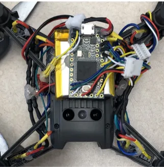
Fig. 3-8 shows the forward mounting of the payload on the bottom of the Tello.

Figure 3-8: Wiring, Micro JST connectors and hot glue with the instrumentation payload on the Tello quadrotor UAV. The Teensy v3.2 Arduino and battery pack are visible. Nose of the vehicle is at the top of the image, and the vehicle’s outer-loop optical flow sensors are near the bottom.

1_{From the center of mass’s perspective, it can also be considered that rotor lift is adjusted to} place center of lift under the center of mass. In either case, the sum of torques is zero at the center of mass during a steady hover.

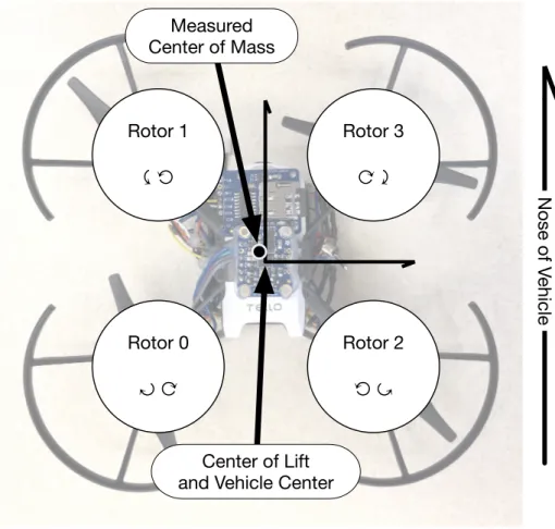
The measured center of mass by orthogonal wire-hang tests was 2 mm forward and 2.4 mm left of vehicle center, as visible in Fig. 3-9. The payload often shifted between flights, however, and this was the one measurement made after the flight tests and after re-securing components with hot glue. The center of mass calculation for each flight test was inferred by torque required to maintain hover.

Rotor 1 Rotor 0 Rotor 2 Rotor 3 Nose of V ehicle Measured Center of Mass Center of Lift and Vehicle Center

Figure 3-9: Tello COM was measured to be 2 mm forward, 2.4 mm left of the vehicle’s geometric center.

By processing flight test data, center of mass is calculated by the axes’ hover torque and ~⌧ = ~r ⇥ ~F . The extremes of results over all test flights are tabulated in Table 3.1.

The vehicle’s battery was initially secured, but became loose after several crash landings. As a result, the payload’s battery (apprx. 23 g) had as much as a centimeter of space to shift between flights. By ~r ⇥ ~F , the battery itself could account for an additional 0.0023 N · m of torque (1.86 mm shift in center of mass) at 1 cm forward.

Table 3.1: Extremes of inferred center of mass, associated hover torque, and distance from geometric center, by axis.

Along Axis Min Distance Min Torque Max Distance Max Torque

ˆ

x 2 [mm] .00247 [N · m] 6 [mm] .00740 [N · m]

ˆ

y -2.42 [mm] .00298 [N · m] 1.62 [mm] .00200 [N · m]

3.3 Data Processing

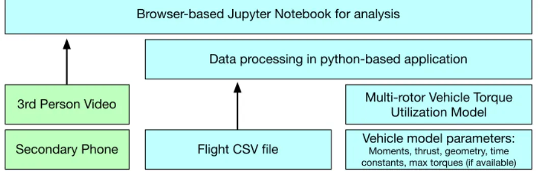
The data is processed primarily with the Pandas and Numpy Python packages and custom object and process-oriented programs for computing control margin. The separation of concerns detailed in Fig. 3-10.

Flight CSV file Vehicle model parameters:Moments, thrust, geometry, time constants, max torques (if available)

Multi-rotor Vehicle Torque Utilization Model Secondary Phone

3rd Person Video

Data processing in python-based application Browser-based Jupyter Notebook for analysis

Figure 3-10: Flight data post-processing diagram.

Each data-recording session was synchronized with at least one video stream to aid in the analysis. One video was recorded from a relevant 3rd _{person perspective,}

another was captured by the vehicle’s on-board camera, where because it lacked time-keeping ability, its feed was rarely used.

In general, video recordings are synchronized to flight logs at rotor spin-up. The processing software determines when rotors are spun-up, and the audiovisual record-ing is reviewed to determine the time interval to shift the data feed.

3.3.1 Revolutions Per Second

RPS was calculated using a sliding window sum of blade passes, divided by the 100

ms window length. The result is the same as a numeric derivative with points from

The resolution is 5 RP S for a sampling frequency of 10 hz. Larger windows give better resolution but at a lower frequency.

3.3.2 Angular Velocity and Acceleration

Angular acceleration was determined by a single difference derivative of angular ve-locity. Angular velocity was available from the IMU directly.

3.3.3 Filtering

Inspection of the Fourier transform of flight test data (Fig. 3-11) led to identification of a 12.5 hz cutoff frequency for roll and pitch rates through a 2nd _{order Butterworth}

low-pass filter. Yaw rates were given a cutoff of 2.5 hz. Zeroth-derivative angle data is only used in the analysis, is not used by the metric. Because of this, zeroth-derivative angle data was not filtered.

Numerical differentiation amplifies noise, but a Fourier analysis of angular velocity data showed that most energy in roll and pitch exists beneath 12.5 hz. Therefore, roll and pitch velocity and acceleration were filtered at 12.5 hz.

The gyroscope yaw rate data had almost all of its energy beneath 2.5 hz, therefore the cutoff was placed at 2.5 hz for yaw velocity and acceleration.

Despite having a Nyquist rate of 5 hz, the 10 hz motor data was found to have substantially all its energy beneath 2 hz. Therefore, motor data was filtered to 2.5 hz before it was used in generating control margin output. This choice also aided in fitting yaw acceleration data in § 3.4.3.

3.4 Sum of Torque Calibration

In this chapter, lift and motor torques are determined to be functions of RP S2_.

Rotor lift was determined by vehicle weight and shown to be a function of RP S2_.

Rotor lift torque then depends on lift and the distance from the axis of rotation considered.

Figure 3-11: Gyroscope rates for a Tello flight, absolute value of the Fourier transform. Identified cutoffs: roll and pitch 12.5 hz, yaw 2.5 hz.

Motor yaw torque is determined by fitting RP S2_{with acceleration ⇥ an estimated}

yaw inertial moment during controlled yaw of the vehicle.

At typical tip speeds of the rotor blades (80-110 m/s), the maximum longitudinal speed of wind supported by Tello (5 m/s) has very little ability to change the angle of attack of the rotors. This study neglects the effects of oblique (non-axial) flow on rotor performance, in favor of a model that requires no information about longitudinal wind velocity.

Torque effects of forward velocity are often canceled on a multi-rotor through sym-metric rotor layout; however, there are effects of wind shadow that are not considered in this study.

3.4.1 Lift Torque by RP S

_Calculation

Rotor lift is first shown to be solely a function of RP S2_{. Lift is defined as a function}

of flow velocity in Eq. (3.2), in a useful form in Eq. (3.3), where Cl is a function

of angle of attack Cl = Cl↵ ⇤ ↵, and V is the rotor-experienced flow velocity, cr is

the cord width at radius r. V is a combination of velocity of the rotor (!r) and the flow induced across the rotor by the pressure differential induced velocity (Ui).

The relationship between RP S and induced velocity is complex, although able to be modeled linearly for Tello.

L = 1 2⇢V 2_SC l (3.2) dL = 1 2⇢V 2 r ⇤ Cl↵↵⇤ crdr (3.3)

Rather than measure and curve fit, lift’s relationship to ! is developed in theory, and then required coefficients are found experimentally. The theory does not fully account for induced velocity, but the linearized model of induced velocity did not produce evidence of substantive errors at this rotor-blade scale.

The magnitude of vertical lift required was calculated with the knowledge that Tello’s rotors point straight up. Other test vehicles with angled rotors may need their weight vectors proportionately scaled to determine necessary rotor-aligned thrust.

V = q

U2

i + (!⇤ r)2 (3.4)

Eq. (3.4) gives velocity as a function of r and w. It’s possible to compute the

induced velocity Ui by equating the momentum change of the flow with the thrust

generated. However, a model is needed to determine Ui without first having thrust.

A model is generated for Ui using values at hover and momentum theory.

Momentum theory with actuator disk theory as described by McCormick in [5] assumes a uniform velocity flow across a rotor. It assumes incompressible flow and well-defined stream tubes into and away from the rotor, which by symmetry makes

the velocity increase at the rotor one half of the downstream increase. This allows for simple physics treatment to determine rotor force by Eq. (3.5), multiplying mass flow and change in velocity.

F = d(m⇤ v)

dt =

m

dt ⇤ v = ˙m ⇤ v (3.5)

Velocity at the disk is halfway between free stream (U1) and downstream (Uexit)

velocities. This can be shown by equating power of momentum change and kinetic energy change, which allows solving for velocity at the rotor disk, as in Eq. (3.6) and Eq. (3.7). Udisk U1 is called induced velocity, or Ui. With 1/2 added velocity as

Ui, the down-steam velocity is U1+ 2⇤ Ui.

P ower = ˙m_⇤ 1 2(U

2

exit U12) = L⇤ Udisk = ˙m⇤ (Uexit U1)⇤ Udisk (3.6)

Udisk =

1

2(Uexit+ U1) (3.7)

Eq. (3.5) with v = 2⇤Ui gives the thrust equation using actuator disk momentum

theory in Eq. (3.8). For a multi-rotor in hover, U1 is 0. Therefore Eq. (3.9) shows

Ui / p L. L = ˙m_{⇤ (2 ⇤ U}i) = ⇢⇡R2⇤ Ui⇤ (2 ⇤ Ui) = 2⇢⇡R2⇤ Ui2 (3.8) Ui = s L 2⇢⇡R2 (3.9)

As a guess towards modeling Ui, suppose Ui / w, Ui = !⇤ ki, Eq. (3.10). Using

momentum theory (Eq. (3.9)), hover lift (weight/4– vehicle mass is 125.7 grams) requires 5.04 m/s flow acceleration. Because hover is done at 325 RP S, parameter ki is identified, ki = 2.47⇤ 10 3 [m⇤ (radians) 1].

Ui = !⇤ ki (3.10)

To see whether the Ui model is correct, a two point validation is utilized through

the lift equation and momentum theory. Given Ui = w⇤ ki, the velocity equation is

simplified in Eq. (3.11).

V =p(!⇤ ki)2+ (!⇤ r)2 = !

q k2

i + r2 (3.11)

This allows an updated model for lift to be built in Eq. (3.12).

dL = 1

2⇢⇤ !

2_(k2

i + r2)⇤ Cl↵↵⇤ crdr (3.12)

But now it’s important to consider ↵. Alpha is the angle of attack, which is the

difference between the local blade pitch and induced velocity angle , as seen in

Fig. 3-12 and expressed in Eqs. (3.13), (3.14).

↵ = ( ) (3.13) Cl= Cl↵⇤ ( ) (3.14) ωr φ V Uᵢ β

Figure 3-12: Effective angle of attack ↵ depends on blade pitch and induced angle .

= tan 1Ui

!r (3.15)

is the induced angle of attack, the angle of the incoming rotor wind relative to the plane of rotation of the rotor. When Eq. (3.15) is substituted into Eq. (3.12), the result is a complete differential form of the lift equation.

dL = 1 2⇢⇤ ! 2_(k2 i + r2)⇤ Cl↵( r tan 1 Ui !r)⇤ crdr (3.16)

Substituting the Eq. (3.10) model for Ui yields Eq. (3.17), where it can be noticed

that ↵ becomes only a function of rotor blade geometry, ↵ = r tan 1 k_ri.

dL = 1 2⇢⇤ ! 2_(k2 i + r2)⇤ Cl↵( r tan 1 !ki !r)⇤ crdr (3.17)

An integration by radius in Eq. (3.18) yields a model of lift that depends only on w2_{. The change in geometry and all other constants are captured in Eq. (3.19).}

L = !2_⇤ Z rtip rroot 1 2⇢⇤ (k 2 i + r2)⇤ Cl↵( r ki r)⇤ crdr (3.18) L = !2 _{⇤ k}lif t (3.19)

If the linear Ui model Eq. (3.10) holds, then Eq. (3.19), which is based on first

principles, is necessarily true. klif t is fit at hover, and

klif t = 7.42⇤ 10 8 [N ⇤ s2 (radians) 1].

The Ui model is linear. If the induced velocity phenomena is linear in RP S, it

is sufficient to check that the model and momentum theory are in coherence at least one other RP S (see limitations § 5.1.4).

The thrust model at 425 RP S predicts 0.529 N of thrust per rotor. By momentum theory Eq. (3.9), this is Uimomentum = 6.60m/s, and by the linear model Eq. (3.10),

425 RP S yields Uilinear = 6.59m/s.

The error here is minuscule, and it is judged unlikely that the underlying Ui is

holds as a relation to !2_{, L = !}2 _{⇤ k} lif t.

Recalling the overall dynamics equation Eq. (2.4), rotor lift torque is ~r ⇥ ~F , which depends on the distance and direction of the rotor from a reference point. Rotors point directly up, and rotor distances from the vehicle geometric center are directly measured. On the Tello, the four rotors are displaced symmetrically, 3.94 cm longi-tudinally (ˆx), 4.32 cm laterally (ˆy). The lift torque equation is found in Eq. (3.20).

Tlif t = ~r⇥ !2klif tzˆ (3.20)

3.4.2 Inertial Moments

For their role in residuals and calibration of motor torque, it is necessary to determine the vehicle’s inertial moments with payload.

Inertial moments of the vehicle are estimated by separately modeling the main body of the vehicle and the rotors, motors and propeller guards, and combining their results.

A stock Tello with battery, rotors and rotor guards is 80 g. With the payload, the vehicle weighs 125.7 g. The body mass alone is 101.86 g, longitudinal length is 6.47 cm, lateral width is 4.84 cm, and height is 3.94 cm, the body’s inertial moment is calculated on each axis as a rectangular box using Eq. (3.21).

Ibody x=

body mass

12. ⇤ (width

2

y + height2z) (3.21)

The rotor (4.9 g), motor blade and propeller guard together weigh 5.96 g. For simplicity they are treated as small spheres with diameter equal to the motor height (2 cm), giving their inertial moments in Eq. (3.22). The distances stated in § 3.4.1 with the parallel axis theorem, Eq. (3.23), gives rotor inertial moments relative to the body coordinate system.

Irotor =

2

5rotor mass⇤ r

Table 3.2: Tello with Payload Inertial Moments at Geometric Center

Axis Inertial Moment

Roll (Ixˆ) 7.85⇤ 10 5 [kg· m2]

Pitch (Iyˆ) 8.68 ⇤ 10 5 [kg· m2]

Yaw (Izˆ) 1.38⇤ 10 4 [kg· m2]

Iparallel axis = Irotor+ rotor mass⇤ distance2 (3.23)

The result of the inertial moment calculations are in Table 3.2.

3.4.3 Motor Yaw Torque by RP S

_Coefficient

Motor torque is the primary means of rotating the Tello quadrotor about its yaw (ˆz) axis (Fig. 3-3). Power equivalence determines the theoretical ⌧motor relationship with

!2_{, which is then fit to data.}

The power from lift and motor torque (⌧motor) is equated in Eq. (3.24) to determine

⌧motor’s relationship with !2 in Eq. (3.25).

P ower = (Lrotor⇤ Ui)out = (⌧motor⇤ w)in⇤ ⌘ef f iciency (3.24)

⌧motor = Lrotor⇤ Ui w_{⇤ ⌘}ef f iciency = ! 3_{⇤ k} lif tki !_{⇤ ⌘}ef f iciency = ! 2_{⇤ k} lif tki ⌘ef f iciency = !2kmotor (3.25)

Motor torque coefficient was fit to yaw acceleration data which determines the corresponding efficiency coefficient.

Determining the motor torque coefficient is not as simple as it was for lift torque, which utilized vehicle weight and directly measurable vehicle geometry. Instead, calibration depends on a demonstrated acceleration through an inertial moment in still air, where the acceleration is known to be a result of the motor torque. That said, by klif t⇤ki, it’s known that the motor torque is at least 5.98⇤10 11[N⇤m⇤s2(radians) 2].

A number of tests were performed in still air, where the vehicle yaws under its

own control. A baseline for the kmotor is found by Eq. (3.26) where spin direction

is ±1 depending on direction of rotation.

For a baseline calibration of kmotor (P⌧motor/P±!2 = I⇤ ↵/P±!2 in still air),

the average value of Eq. (3.26) was taken over four still-air hover yaw actions.

Thir-teen seconds of applicable data were used, which excludes intervals whereP±RP S2

crosses zero. kmotor = Izˆ⇤ ↵yaw Pmotors i RP S2i ⇤ spin directioni (3.26) This baseline calculation is skewed initially by low (close to zero) P±RP S2 seg-ments, and segments with low ↵. Therefore, kmotor is manually adjusted such that at

peak torque (min or max P±RP S2) the quotient of yaw torque match, Eq. (3.27),

is equal to one (= 1).

yaw torque match = Izˆ⇤ ↵yaw

kmotor⇤P±RP S2

(3.27) kmotor is found to be 1.41 ⇤ 10 10 [N ⇤ m ⇤ s2(radians) 2]. Fig. 3-13 contains the

Figure 3-13: Yaw Torque Match ⌘ Izˆ⇤ ↵yaw/(kmotor ⇤P±RP S2). Vehicle torques

itself in still air. There is a minor external interaction with a guide cord at 1m:29s.

Match is not reliable asP±RP S2 approaches zero.

Motor Torque Efficiency Cross Check ⌘ef f iciency =

(Lrotor⇤ Ui)out

(⌧motor⇤ w)in

= .424 (3.28)

With a diameter 3.97cm and hover at 325 RPS and Ui = 5.04 m/s, the efficiency

found by Eqs. (3.10), (3.19), (3.25), in Eq. (3.28), ⌘ef f iciency = .424, is in coherence

with McCormick [5] (Fig. 5-1) who predicts propeller efficiencies between 0.2 and 0.64 for the advance ratio found in Eq. (3.29).

Jhover =

Ui

RP S⇤ R =

5.04

Table 3.3: Max Torque Values Identified

Axis Count Mean Std. Dev Max Torque

Roll 24 .00945 .00866 0.0268 [N · m]

Pitch 24 .00572 .00371 0.0131 [N · m]

Yaw 24 .000699 .000218 0.00114 [N · m]

⌧motor is !2⇤ kmotor.

3.5 Calculating Max Roll, Pitch and Yaw Torque

Six full flight sessions, 21.6 minutes of flight data, were examined to estimate maxi-mum roll, pitch and yaw for the control margin metric. Sessions contained a variety of flight behavior, including altitude-varying maneuvers.

Each flight session was split into two equal length parts and the minimum and maximum of rotor-expressed torque was tabulated for each part. The absolute value of all minimums and maximum were tabulated, and the mean (µ) and standard deviation ( ) was calculated by control axis.

Adding two standard deviations to mean was chosen to suppress false positive loss of control margin for this study, Eq. (3.30). As a result, the over-estimate requires residuals to degrade control margins to zero or below in many cases.

⌧max = µmax torque+ 2⇤ max torque (3.30)

Table 3.3 contains the session statistics, including the max torque values identified. The maximum torque on any vehicle axis is a factor of current lift trim and the relative severity of all errors as judged by the inner control loop of the multi-rotor vehicle. It is possible that maximum torques represent a statistical distribution. If so, with additional data it may be possible to assert probability characteristics for false positives of loss of control.

3.6 Natural Response Time Constant Identification

To determine the parameter for the ! residual, multiple measurements are made and a two standard deviations technique is employed for an over-estimate of each axis’ natural time constant, tc. Per Eq. (2.12), tc/4 is the time period during which the

vehicle would be expected to zero its velocity in order to return to maximum bounce back within tc.

The actual time constant of the vehicle is difficult to measure because of coupling between roll and pitch, lift coupling, wind coupling or external body (e.g. a string) coupling. However, compared to max torque which depends on system state, there is a true natural frequency by axis. With enough measurements, it would be possible to use the mean of the measurements. However, to reduce false positives associated with incorrectly high torque in the residual, two standard deviations is again added to the mean to find tc.

To measure the natural frequency, videos of the collected data are searched for rejections of impulse-type disturbances. The quadrotor was required to not “visibly” lose control, being required to substantially maintain position during that rejection. Qualifying disturbances were mostly found in Air Jet Impulse Tests (§ 4.1) and Phys-ical Torque Tests (§ 4.2), although two yaw events also met this criteria during an Outdoor Environment Test (§ 4.4).

Fig. 3-14 shows the measurement process for a roll and pitch event during a Physical Torque Impulse Test. At each event, the more clearly defined sinusoid of degrees or angular velocity is measured, either from peak to peak, or from peak to trough. The measured value is scaled into seconds per oscillation for the time constant from that sample. Results of the measurements can be found in Table 3.4.

Figure 3-14: Roll and pitch response period identification during a Physical Torque Impulse Test.

Table 3.4: Natural Time Constant Periods Identified

Axis Count Mean Std. Dev Time Constant

Roll 5 .410 .139 0.689 [seconds]

Pitch 4 .400 .151 0.703 [seconds]

Chapter 4

Results

The tests were structured to evaluate whether control margin is an indicator for loss of control.

Indoor flight tests were conducted in a closed hangar environment with only a HVAC system circulating air. Test flights lasted roughly four to five minutes with the payload, whereas an unmodified Tello has approximately twelve minutes of flight time per battery.

Tests were video recorded from a third person camera with a view of the scene where the vehicle would be operating.

The takeoff procedure of the vehicle was complicated by a bulky payload and a forward center of mass. As a consequence, the vehicle was hand launched in a fashion characterized by gradual reduction of the support on the heavy side of the vehicle. The third party Android App ‘TelloFPV’ was used to control the vehicle, as it was quicker, more reliable and had better controls than the manufacturer’s Tello App, and allowed the automatic capture of first person video upon the beginning of the flight.

Usually, remote control was used only to move the vehicle into disturbances, repo-sition into the frame of the third person camera, or to reporepo-sition hover after a loss of control.

The Tello with payload was found to have very weak yaw authority, occasion-ally losing yaw authority with very minor disturbance. This effect may have been

exacerbated by battery depletion.

This said, there was no indication that the vehicle was confused about its attitude at any time. Even when yaw loss of control happened, the vehicle would respond to attitude control inputs relative to the direction the pilot had faced it prior to the loss of yaw control.

4.1 Air Jet Impulse Test

In this test compressed air at approximately 100 psi was released from a shop air compressor under the Tello in hover, Fig. 4-1. The nozzle was approximately 5 mm in diameter, and the air was released no more than a foot (30 cm) away. The nozzle was aimed at the rear left rotor of the vehicle so as to provide both roll and pitch impulses. Nose Tail Tail Nose ẑ x̂ Air Jet Pitch (-) and Roll (+)

Air Jet Impulse Test

jets into left tail corner

Figure 4-1: Setup of Air Jet Impulse Test. Compressed shop-air jets released into left tail corner of vehicle (under R0, Fig. 3-1) from a distance of about one foot.

Fig. 4-2 shows the result of the vehicle being exposed to two different jets, with a hover and repositioning period between. The jets are clearly visible at 1m:04s and 1m:12s. Both jets blew the vehicle out of its hover position; as a result of the first jet, the vehicle flew further away.

Figure 4-2: Air Jet Impulse Test. Two air impulse jets causing pitch loss of control, which is indicated for pitch. The first loss of control was deeper than the second and caused the vehicle to lose more position.

Pitch margin in response to each jet is shown degraded below 0, indicating loss of control. As expected, the first jet on the vehicle is characterized by a greater loss of control margin in pitch than the second. This suggests that the metric correlates lower values with greater loss of control.

In response to the first jet, loss of roll control is not indicated by loss of roll control margin. Despite having a visibly higher attitude change over the same period as pitch, roll control margin is only degraded to about 0.5. First, Table 3.3 shows max torque for roll is twice that of pitch. This is attributable to vehicle geometry and the standard deviation of the roll axis’ max torque.

First, the vehicle has a larger lever arm for roll than for pitch. Second, the vehicle’s y-axis center of mass varied between flights, increasing the standard deviation of maximum roll torque. The dependence of max torque on center of mass exists due to the control system’s integral-of-error compensation of attitude errors from off-center center of mass. Additionally, flight tests more often stressed the pitch axis than the

roll axis, contributing to a larger standard deviation for maximum roll torques. The roll axis’ two times higher max torque, coupled with 10% lower inertial mo-ment (than pitch) yields a smaller margin degradation. It’s also important to consider relative change from hover control margin. In this context, the 1.2 drop in pitch mar-gin compared to the 0.5 drop in roll marmar-gin bemar-gins to make sense.

The over-estimate technique was designed to reduce false positives. Here it does, although a tighter correspondence is, in this case, desired for roll.

Further, max torque for roll and pitch control is, in reality, coupled in some scenarios. Simultaneous max roll and pitch control inputs may result in a diamond formation of thrust on the quadrotor’s rotors, which decreases total torque output for each flight axis. The vehicle control system decides how the commands are mixed.

The vehicle was indicated to have roughly 30% pitch utilization (margin 0.7) during the hover period between jets. Based on a max pitch of 0.0131 N·m (Table 3.3), this represented 0.00393 N ⇤ m of pitch torque. This quantity could be accounted for by the standard (measured) .00247 N ⇤m (2 mm) forward center of gravity and .00146

N _{⇤ m from an approximately half-centimeter forward loose battery as explained in}

§ 3.2.1.

4.2 Physical Torque Test

4.2.1 Physical Torque Test #1

The physical torque test had a tether tied about the nose (camera side) of the vehicle. The tether was used to put direct torque on the vehicle through a skyward pull, while the vehicle was at hover.

Data collected for this test can be found in Fig. 4-4. The vehicle is exposed to two physical torques. The first, at 3m:38.25s, is a smaller disturbance than 3m:40s. Both cause positional offset, suggesting loss of control, but the latter is a much stronger event, where the vehicle loses substantial position. At 3m:40s, the yaw axis is also accelerated during the tug, leading to degraded margin on the yaw axis.

Physical Torque Test #1

tether attached to both nose propeller guards Nose Tail Nose Tail ẑ x̂ Tether Pitch (+)

Figure 4-3: Setup of Physical Torque Test #1. Physical pitch-up impulses by tether attached on the nose-side of Tello.

In the first moment of the first pitch-up impulse, the torque due to gravity is cancelled by a gradual up-pull on the tether. Next, the impulse is made, angle and velocity increase, and control margin is degraded below zero.

Figure 4-4: Physical Torque Test #1.

study, indicative of a far forward center of gravity. The vehicle was indicated to have roughly 50% baseline pitch utilization (control margin 0.5) during the hover between physical torques. Based on a max pitch of 0.0131 N · m (Table 3.3), this represented 0.00655 N ⇤ m of pitch torque. This quantity could not be entirely accounted for by the standard 0.00247 N ⇤ m (2 mm) forward center of gravity and 0.0023 N ⇤ m from a one cm forward loose battery as provided for in § 3.2.1.

The battery was moved slightly forward prior to the test in an attempt to move it out of the view of position-keeping sensors. Video review confirmed that the battery was likely forward during this test; however, it would have needed to move 1.77 cm to fully account for this torque, much more than the 1 cm afforded. With the forward battery torque subtracted, if the tether weighed 1 gram including the tape used to hold it in place, the tether would need a lever arm of 18 cm to present the remaining .00178 N ⇤ m. As it was, the tether weighed less than a gram, most of the weight was held by a human most of the time, and the attachment point to the rotor guards was 8 cm from geometric center.

The most plausible explanation is the tether hovering slightly under the front rotors’ flow, which may have caused enough drag to explain the remainder of the hover torque. This was the only test where the center of mass (requiring torque utilization at hover) was on the same side where the tether was placed. In fact, the Physical Torque Test #2 (§ 4.2.2) has one of the lowest hover utilizations, at 25%, and the tether is under the rear flow. This was the explanation accepted.

At 3m:38s the control margin of pitch actually increases before dropping. This is connected with a very slight upward force on the tether before the actual impulse strikes, and is followed by a degraded margin beneath zero before 3m:38.50s. It is not expected that margin should increase before sinking beneath zero. The concern is that positive change in margin would ideally not be a predictor of control loss. Rather, it could make more sense for only negative change in margin to indicate impending control loss. A solution by computing torques about the center of mass is discussed in § 5.1.3.

4.2.2 Physical Torque Test #2

The test setup in Fig. 4-5 has a tether pulling up on the opposite sense of the vehicle’s pitch axis, at the tail-end of the vehicle, torquing it while having the vehicle climb substantially, reducing lift trim.

The progressive degradation of margin with increased pitch torque utilization simulates a steadily increasing shear wind. Different than winds, which don’t have intentional feedback characteristics1_{, in this test, the more the vehicle spins-down}

rotors, the more torque acts on the vehicle.

Nose Tail Nose Tail ẑ x̂ Tether Pitch (-)

Physical Torque Test #2

tether attached to both tail propeller guards

Figure 4-5: Setup of Physical Torque Test #2. Physical pitch-up step function by tether attached on the nose-side of Tello.

Data collected in this test is presented in Fig. 4-6. The vehicle continues to be supported at or slightly above its desired altitude until torque plateaus and lift trim decreases the vehicle into loss of control.

Yaw accelerations were incidentally imparted during the session, as evidenced by the control margin degradation. The hover pitch lift trim is 75% for this position of tether, which was one of the lowest pitch utilizations at hover.

Figure 4-6: Physical Torque Test #2. Physically pulling-up vehicle pitch from tail-end of Tello. This example simulates a progressive torquing updraft. Note: a momentary IMU discontinuity at 6m:40s was not removed by filters.

Given the substantial (simulated) updraft, the cm metric may possibly record a false positive for a short period at 6m:30s, while the vehicle is still maintaining position and attitude control, but torque utilization was higher than max pitch torque. The metric registered loss of control margin at the mean plus two standard deviations max torque value, calculated from multiple flight sessions (Table 3.3). However, the disturbance in this test was of a level not ordinarily encountered in the flight data.

At about 6m:36s, lift trim hits a minimum, and pitch torque hits its maximum, with control margin resting at -0.75. As pitch torque was maximized, the vehicle no longer had the ability to sustain an additional pitch disturbance, and an apparent self induced oscillation beginning at 6m:37s leads to the vehicle’s total loss of control. The vehicle shuts off shortly thereafter at 6m:44s due to a safety feature in regard to runaway angle.

The metric was an indicator of loss of control, although max torque was inaccu-rately small for the initial loss of control in this case. As a result, the metric did not perform as an over-estimating sufficient condition as intended. That said, the metric performed as expected relative to the max torque parameter. In all likelihood, if

the vehicle were not tethered it would have compounded position errors long before, indicating a typical loss of control event.

Modeling the relationship between max torque and lift trim could be expected to improve the overall accuracy of the metric in this low lift condition. The discussion section § 5.1.2 further discusses the relationship between max torque and lift trim.

4.3 Turbulent Vertical Flow Test

In this test the Tello was flown in a room with a large box fan facing vertically. The vehicle was flown into the vertical fan flow several feet above the fan, as described in Fig.4-7. Nose Tail Nose Tail ẑ x̂

Large Shop Fan

Figure 4-7: Setup of Turbulent Vertical Flow Test. The vehicle is flown over the vertical-facing shop fan.

Data collected for this turbulent vertical flow test can be found in Fig. 4-8. The vehicle is in the flow of the fan from 2m:32s to 2m:36s. Yaw motor torque is zero until approximately 2m:36.50s, where it is finally brought into use. At 2m:34.50s the vehicle nearly reaches 1000 degrees/s rotational velocity, or 2.75 revolutions per second. The entirety of the rotational velocity is cancelled, from 800 degrees/s to 0

degrees/s from 2m:36s to 2m:37s.

The peak RPS (2.75 hz) is higher than the filter frequency for motor readings, which suggests the torque readings could be missing important higher frequency

in-formation. As a result, more credence should be given to changes in velocity in this test as evidence of control system actuation than to motor torque indications, which should instead be thought of as a running-average2_.

The flow was considered turbulent, and it is noted that the vehicle yawed clockwise (looking down on the vehicle) the majority of times (all but one brief rotation counter-clockwise). The vehicle was able to pass through the flow directly without spinning, and there was a center point over the fan where the vehicle could hover without spinning. These observations suggest the quadrotor interacted with the flow itself.

Both roll and pitch are articulated throughout the test, and the vehicle appeared to be adjusting its attitude throughout the spin, especially between 2m:32.5s and 2m:36.5s.

Figure 4-8: Turbulent Vertical Flow Test. A high angular velocity yaw loss of control after the vehicle was positioned over a large vertical-facing fan.

This event exemplifies the residual portion of the control margin metric. The lead up to peak yaw rate at 2m:34.25s marks the point of minimum control margin. At 2m:35s, the vehicle is experiencing large acceleration opposite to the yaw rate, marking a local maximum of control margin, at roughly cm -0.5. There is one more

2_{Admittedly, the control system does have a small amount of help in roll and pitch by the passive} stability of a disk with momentum about the world ˆz axis [6].

increase in yaw rate which drops the control margin to about -4.75, immediately before the final deceleration brings margin back into control.

The final deceleration from 800 degrees/s takes almost exactly one second, which would indicate a time response of 4 seconds. In reality, tc is 1.47 seconds (Table 3.4),

which made it 2.72 times longer than a controlled response.

There are almost no times during this experiment where yaw angular acceleration is zero; however, 2m:34s is the closest with less than 100 degrees/s2_{. During this}

time control margin is about -3.5, which is the presumed angular velocity residual component. At all other times until yaw torque begins, the control margin is the combination of the effects from angular acceleration and velocity residuals.

Roll and pitch both maintain indicated control during the entire test.

That the vehicle waited until 2m:36.5s to begin yaw torque may be attributable to the mixing priorities of the control system. Until 2m:36.5s the vehicle experienced substantial roll and pitch upsets, presumably because of the turbulent flow. With the Tello, the co-rotating rotors of the diagonal and the perpendicular diagonal increase and decrease for yaw motor torque control (See Fig. 3-1). This allows isolation of yaw control from pitch and roll. The behavior increases the ease of piloting, but also means full yaw authority may not exist with full roll and pitch authority. This is especially true when flying close to max RPS or when large roll and pitch inputs are desired.

Compared to roll or pitch, yaw authority loss will not result in the physical upset of the vehicle. Further there was piloting evidence that the vehicle did not lose spatial orientation easily and vehicle yaw “confusion” was ruled out. As a result, the delay of yaw torque was most likely attributable to the prioritization of roll and pitch errors until the external roll and pitch disturbance was removed.

Review of common PID controller implementations [1] confirmed a mechanism for action of this behavior is thrust saturation. Simultaneous pitch and roll commands are likely to saturate two of a quadrotor’s rotors on a diagonal, at maximum and at minimum. By clipping to maximal values, an additional or subtracted yaw command would not have any effect on rotor setpoints. If designed to maintain lift trim, the