Publisher’s version / Version de l'éditeur:
Atmospheric Measurement Techniques, 9, 2, pp. 619-630, 2016-02-24
READ THESE TERMS AND CONDITIONS CAREFULLY BEFORE USING THIS WEBSITE. https://nrc-publications.canada.ca/eng/copyright
Vous avez des questions? Nous pouvons vous aider. Pour communiquer directement avec un auteur, consultez la première page de la revue dans laquelle son article a été publié afin de trouver ses coordonnées. Si vous n’arrivez pas à les repérer, communiquez avec nous à [email protected].
Questions? Contact the NRC Publications Archive team at
[email protected]. If you wish to email the authors directly, please see the first page of the publication for their contact information.
NRC Publications Archive
Archives des publications du CNRC
This publication could be one of several versions: author’s original, accepted manuscript or the publisher’s version. / La version de cette publication peut être l’une des suivantes : la version prépublication de l’auteur, la version acceptée du manuscrit ou la version de l’éditeur.
For the publisher’s version, please access the DOI link below./ Pour consulter la version de l’éditeur, utilisez le lien DOI ci-dessous.
https://doi.org/10.5194/amt-9-619-2016
Access and use of this website and the material on it are subject to the Terms and Conditions set forth at
Software to analyze the relationship between aerosol, clouds, and
precipitation: SAMAC
Gagné, S.; MacDonald, L. P.; Leaitch, W. R.; Pierce, J. R.
https://publications-cnrc.canada.ca/fra/droits
L’accès à ce site Web et l’utilisation de son contenu sont assujettis aux conditions présentées dans le site LISEZ CES CONDITIONS ATTENTIVEMENT AVANT D’UTILISER CE SITE WEB.
NRC Publications Record / Notice d'Archives des publications de CNRC:
https://nrc-publications.canada.ca/eng/view/object/?id=94b41542-eff9-4a96-9587-74e5aaba03b8 https://publications-cnrc.canada.ca/fra/voir/objet/?id=94b41542-eff9-4a96-9587-74e5aaba03b8
www.atmos-meas-tech.net/9/619/2016/ doi:10.5194/amt-9-619-2016
© Author(s) 2016. CC Attribution 3.0 License.
Software to analyze the relationship between aerosol,
clouds, and precipitation: SAMAC
S. Gagné1,2,a, L. P. MacDonald1,3, W. R. Leaitch2, and J. R. Pierce1,3
1Department of Physics and Atmospheric Science, Dalhousie University, Halifax, B3H 3J5, Canada 2Environment Canada, Downsview, Toronto, M3H 5T4, Canada
3Department of Atmospheric Science, Colorado State University, Fort Collins, CO 80523, USA anow at: National Research Council Canada, Ottawa, Ontario, K1A 0R6, Canada
Correspondence to:S. Gagné ([email protected])
Received: 30 January 2014 – Published in Atmos. Meas. Tech. Discuss.: 10 April 2014 Revised: 2 February 2016 – Accepted: 2 February 2016 – Published: 24 February 2016
Abstract. The analysis of aircraft-based measurements of clouds is critical for studies of aerosol and of clouds. Many such measurements have been taken, but it is difficult to com-pare such data across instruments, flights and campaigns. We present a new open-source software program, SAMAC (Soft-ware for Airborne Measurements of Aerosol and Clouds), that may enable a more systematic and comparable approach to the analysis of aerosol–cloud–precipitation data. The soft-ware offers a cooperative and reproducible approach to the analysis of aircraft measurements of clouds across cam-paigns. SAMAC is an object-oriented software program in which a cloud is an object; all the data related to a cloud is contained in the cloud object. The cloud objects come with built-in methods and functions that allow for the quick generation of basic plots and calculations, SAMAC provides a quick view of the data set and may be used to compare clouds and to filter for specific characteristics. Other re-searchers can readily use already submitted algorithms once their data is placed in the cloud structure provided, and they can contribute their own algorithms to the software for oth-ers to see and use. This approach would improve compara-bility, reproducibility and transparency by allowing others to replicate results and test the same algorithms on differ-ent data. SAMAC can be downloaded at https://github.com/ StephGagne/SAMAC/releases.
1 Introduction
The links between aerosol, clouds, and precipitation are of-ten referred to as one of the least understood, and some of the most important processes by which humans affect the Earth’s climate (IPCC, 2007). Aerosols, clouds, and precip-itation are described in global climate models (GCMs) us-ing parametrizations (e.g Nenes and Seinfeld, 2003; Mor-rison et al., 2005). The parametrizations are validated and constrained using remote sensing or direct airborne mea-surements (see e.g. Zhang et al., 2013), and have also been developed based on these measurements (e.g. Boucher and Lohmann, 1995). Measurements of aerosols, clouds, and pre-cipitation in concert are crucial to better constrain global climate models. Satellite observations are very helpful in the study of aerosol–cloud–precipitation interactions because they cover large and diverse geographical areas, but they are not without some biases (e.g. they generally cannot sample co-located aerosols and clouds). Therefore, airborne in situ measurements are a necessary part of the improvement of the aerosol and cloud processes in GCMs.
Airborne measurements of aerosol–cloud–precipitation interactions have been performed on different cloud types, and in different areas around the world (see e.g. campaigns such as RICO (Rauber et al., 2013), VAMOS-VOCALS (Wood et al., 2011), or MASE (Lu et al., 2007)). In many cases, these measurements were performed using an aircraft tracing a single path through clouds (e.g. Leaitch et al., 1996; Johnson et al., 2000; Schmid et al., 2000; Sollazzo et al., 2000; Kleinmann et al., 2012). This measurement method
makes data analysis difficult because the relevant parame-ters are measured at different time intervals and at different places in 3-D space and subject to variability in the condi-tions at the time (e.g. clouds may be in different stages of their life cycle during sampling). Further, the aerosol effects, while important, may be subtle relative to other aspects of the cloud life cycle. Another difficulty of airborne measurement is the lack of standardized instrumentation, data processing and analysis. While, during a given measurement campaign, all the clouds are likely to be measured with the same set of instruments, it may not always be possible to perform the same calculations for all of them. Between campaigns and research groups, analysis of clouds can vary even more. Im-proving the traceability and comparability of data analysis would help with providing modellers with more transparent and comparable data.
The creation and use of an open source standardized database structure and software would allow researchers from different institutions to compare their measurements with those of others more easily. Moreover, a basic quan-tity, such as the concentration of below-cloud aerosols, could be calculated using exactly the same technique (algorithm), making the quantity more comparable across various clouds, campaigns, and in the literature. Such software could also improve analysis speed by producing basic plots and calcula-tions so that the analyst can visualize multiple aspects of the measured clouds rapidly and then decide on the next analysis steps to take. Sharing algorithms between researchers also saves coding time for all participants in addition to providing a good basis for comparison.
For this kind of software and data structure to be benefi-cial for the whole research community, it should be freely available for all researchers and easy to modify to fit their needs. The modifications should be traceable and reference-able. The software should hence be written in a free, cross-platform programming language, be open-source and under version control. The advantages are the following:
a. it can be modified by the users in order to better fit their needs;
b. when a user makes a modification that could be useful to others or that makes the software more flexible, the modification can be included in the next public release; c. when improvements are made to functions (a predefined routine), version control ensures that the old function can still be retrieved and used if needed. This way, cal-culations are reproducible (as long as the function name and the software version is mentioned in publications); d. although there is a need for a coordinator overseeing
the quality and release of new versions of the software, participative programming under version control means that improvements can be made gradually by users who need these improvements, sharing the effort between users.
In this paper, we present a data structure for cloud measure-ment data and analysis software, SAMAC (Software for Air-borne Measurements of Aerosol and Clouds), that attempts to answer the concerns and fulfil the specifications discussed above. In this work, we first give an overview of SAMAC’s capabilities after which we explain our coding choices. We then give basic instructions and specify the requirements to use and modify the software. Next, we describe the current structure and the different function types in the software. Fi-nally, we illustrate the uses of SAMAC with IPython, an in-teractive python shell, using data from the Canadian SOLAS 2003 campaign (Gagné et al., 2016).
2 Overview of software capabilities
Software processing and visualizing airborne measurements already exist, and some are complementary to SAMAC. The ADPAA (Airborne Data Processing and Analysis, writ-ten in IDL and C-shell) package developed at the Uni-versity of North Dakota, “is intended to fully automate data processing while incorporating the concept of miss-ing value codes and levels of data processmiss-ing.” (Delene, 2010). The EGADS software (EUFAR General Airborne Data-processing Software, written in Python) designed at EUFAR is “a toolbox for processing airborne atmospheric data” (EUFAR-EGADS, 2016), https://code.google.com/p/ eufar-egads/). EGADS aims to be a community-driven soft-ware for processing airborne data and already provides many data-processing routines for common airborne instrumenta-tion. MMM (Mesoscale and Microscale Meteorology) Soft-ware, provided by UCAR and Java-based includes “data analysis packages for radar, aircraft, surface mesonet, sound-ing and gridded data” (Atmospheric Science Software Ap-plications – UCAR Community Tools, 2009; https://www. ucar.edu/tools/applications_desc.jsp). Unidata (2016) also provides a visualization tool called IDV (Integrated Data Viewer, Java-based) which can be used to display geoscience data (Unidata | IDV, https://www.unidata.ucar.edu/software/ idv). All of these available software programs are focused on earlier analysis, data correction or pre-processing. With SAMAC, we propose to take the community effort to the next level of analysis of airborne cloud measurements.
SAMAC was given a flexible and adaptable design which makes it well-suited to support cooperation among researchers. Adding an algorithm (called a function) to SAMAC is fairly easy, and other researchers can see the source code to review it and can use it directly on their own data using SAMAC. With reproducibility of results being a concern in the scientific community in the recent years (Na-ture Editorial, 2014; Easterbrook, 2014), a version-controlled open source code would address these concerns while de-creasing the likelihood of bugs in the code by virtue of hav-ing multiple users reviewhav-ing the code.
In addition to the algorithms provided by other users, SAMAC already has a number of methods and functions (routines) that allows users to rapidly visualize their data, ex-ecute standard operations, and add practical information to their data. In this section, we present a brief overview of the software’s features.
In order for the methods and functions to work on one’s data, the measurement data must be filled in the cloud ob-ject structure of SAMAC. Guiding software is available with SAMAC but may need to be modified to fit different data/file formats. Some tips are available on the SAMAC website. Once the data is placed in the cloud structure of SAMAC, some basic methods and functions become available to users, along with functions developed by other users and gradually added to the software package.
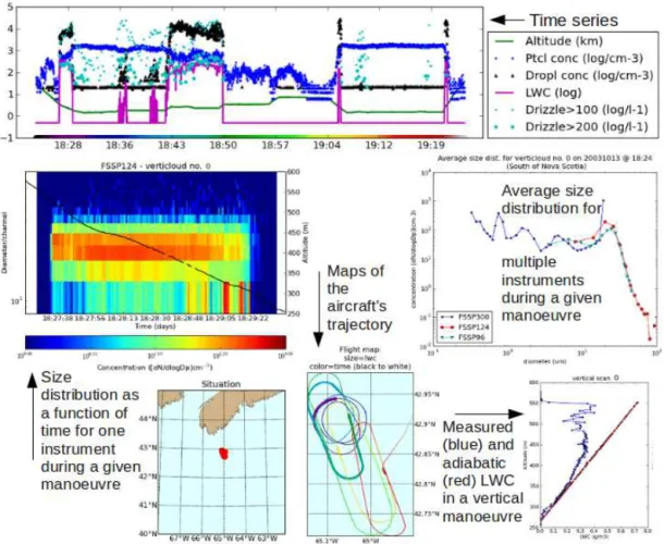
SAMAC comes with a set of figure-generating functions that include time series, vertical profiles and adiabatic liq-uid water content. Some examples from these plots can be found in Fig. 1. A figure, or many figures in certain cases, can be generated using only one line of code that calls the plotting function. The code looks for the relevant data in the cloud structure and no further input is needed from the user. The figure-generating functions that are available in this ver-sion of the software include a time series, maps of the air-craft trajectory, various size-distribution figures, and differ-ent types of vertical profiles (with altitude as the y axis).
This software also comes equipped with a suite of calcu-lation functions. For example, with a single-line command, a user can get the liquid water path, the average size distribu-tion within a chosen aircraft manoeuvre or flight leg, an av-erage cloud droplet number concentration, and more. As we later show in Sect. 5.2, it becomes very easy to make plots that aggregate results from many clouds, controlling for cer-tain characteristics.
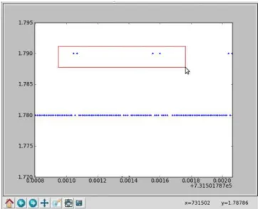
There are also a few “interactive” methods. Some are based on users clicking on a figure to provide information to the software. To define the time period of a manoeuvre for example, the user can either determine the times and in-sert them manually into the structure of the cloud instance, or use a specially designed interactive function and click on the beginning and end time of the manoeuvre on a time series plot (top panel in Fig. 1). The same principle can be used to define the base and top of a cloud. The clicking principle is also used in a method created to help mask unphysical, er-roneous or dummy data (Fig. 2). In this method, the points within a rectangle defined by the user become masked af-ter receiving confirmation. Another category of inaf-teractive methods require the user to answer questions on the prompt. For example, there is a method to assess the quality of liquid water content profiles that asks users to enter quality flags for profiles.
3 Programming techniques
We created and developed SAMAC in order to process surements of clouds spanning more than 30 years. The mea-surements had taken place on several different measurement campaigns with varying cloud types and the instrumentation changing from one campaign to another. In order to compare the different clouds with each other, standard structure and calculation techniques had to be implemented. The structure had to be flexible enough to allow adding new data in case some instrument’s data had not been foreseen or were not in the original data set. Another important feature, was that if the original data had to be corrected or re-calibrated, all the related calculations would be corrected automatically: the user would not need to track down the repercussions of this change, instead it would be done by the software itself.
It was decided that object-oriented programming would be the best way to satisfy all these conditions. We define cloud object as the overall class (or type of object) we use to repre-sent measured clouds, and a cloud instance as a particular individual cloud of the cloud object class. Each cloud in-stance of a cloud object is a measured cloud in which the data (e.g. time, altitude and cloud droplet concentration), and a few basic subjective cloud characteristics (e.g. envi-ronment type and cloud type) would be stored in a struc-ture. Object-oriented programming also allows for methods associated with an object. All cloud instances share the data structure and methods associated with cloud objects. Meth-ods are procedures that can be performed on an object (or more precisely, on the data in each instance, Beazley, 2009). The method can either change the instance itself or simply use the data in the instance to return an output. In the case of SAMAC, methods that modify the cloud instances are found in the class file and functions that do not modify the cloud instances are found separately from the class file.
We have chosen Python as a programming language for SAMAC mainly for these reasons:
a. Python is a free, open-source, cross-platform, high-level programming language;
b. Python is already used among researchers in the Earth sciences (Lin, 2012; Perkel, 2015);
c. Python has a very clear, readable syntax (Python Pro-gramming Language, 2013);
d. new scientific programming packages in Python are re-leased on a regular basis (Yarkoni, 2013);
e. Python’s NumPy module provides Masked Arrays (2013), which allow for the masking of unphysical or missing/dummy data without having to delete or overwrite them with flag values. Masks are preserved through calculations (masked inputs give masked out-puts);
Figure 1.Figures generated by a selection of functions available in SAMAC. On the first row, the time series shows a selection of data as a function of time. This function is used to provide an overview of a particular flight and the aerosol and cloud measurements (more detail on the time series in Fig. 4a). On the left-hand-side figure of the middle row is a size distribution as a function of time during a vertical profile manoeuvre. The colour represents the concentration and the black line the altitude. On the right-hand side, the average size distribution is plotted for a selection of instruments for one manoeuvre. The two figures on the middle row can be generated for any size-distribution instrument and manoeuvre. The maps on the bottom row show a general situation map and a zoomed-in trajectory of the aircraft in the cloud. The size of the points correspond to the liquid water content. The colour corresponds to the time bar at the bottom of the time series (more details on the maps in Fig. 4b). Finally, the figure in the lower right corner displays a profile of the measured and adiabatic liquid water contents.
f. Python’s object-oriented programming allows for many types of methods bound to the object and functions that can interact with the object;
g. Python’s SciPy modules (SciPy.org, 2013), particularly NumPy, Matplotlib (2016), Hunter (2007) and Pandas are similar to Matlab and R which are two additional programming languages that are widely used in the Earth sciences. Python also has an interface module with R: RPy (RPy: a simple and efficient access to R from Python, 2013).
The software was tested using Python 2.7.1 with Matplotlib 0.99.3, NumPy 1.5.1, SciPy 0.8.0, and Basemap 1.0.1 on Linux Mint 11; with Python 2.7.3 with Matplotlib 1.1.1, NumPy 1.6.2, SciPy 0.10.1, Basemap 1.0.5 and h5py 2.0.1-2 on Linux Mint 14; and with Python 2.0.1-2.7.3 with Matplotlib
1.3.1, NumPy 1.8.0, SciPy 0.13.0, Basemap 1.0.7 and h5py 2.2.0 on OSX 10.9.1 (Build 13B42).
Because the software was designed to handle cloud flex-ibly (with different instrument types and number of instru-ments, different aircraft trajectories and series of manoeu-vres, etc.), SAMAC is ideal for use and modification by other research groups to compare algorithms. Once the data is placed inside the cloud instance, the methods and func-tions can be applied right away. The use of SAMAC by other research groups should serve to increase comparability, test each others’ algorithms on one’s own data, and speed up data analysis by using other researchers’ algorithms with-out a need to adapt the code. Moreover, shared open-source software makes data analysis more transparent, and possible mistakes are more likely to be spotted and corrected (Challet and Le Du, 2003; Barnes, 2010; Merali, 2010).
Figure 2.This is an example of an interactive method. In this case, the method asks the user to choose a data type to display. The user can then choose to use an automatic outliers removal tool or to zoom in and select the points that need to be masked with a few clicks of the mouse. Here, the points in the red rectangle will be masked when the user confirms it.
SAMAC 1.0.0 can be downloaded at https: //github.com/StephGagne/SAMAC/releases (http: //dx.doi.org/10.5281/zenodo.35730) in the preferred data compression format by clicking on the source code button. SAMAC will work on any platform provided Python 2.7 and the modules listed in the wiki pages are installed. Python is a free cross-platform programming language. Documentation material is available on the wiki pages (book icon, https://github.com/StephGagne/SAMAC/wiki). It includes a description of the SAMAC cloud object structure, a description of the methods and functions associated with cloud objects, and a guide on how to create and populate a cloud object. It also includes an example cloud object with which to explore SAMAC. This example cloud, despite similarities, is not the same cloud that is presented in this manuscript. Git is used for version control. To participate in improving the software and contributing algorithms, a user needs to have an account on GitHub (2016). A GitHub tutorial is available at https://help.github.com/. To contribute a new algorithm, one can contact the software coordinator(s) through the “Issues” section. That same section can also be used to report any bugs or to suggest improvements.
SAMAC falls under the protection of the GNU General Public License version 3. This license allows scientists to use the code in SAMAC and contribute new algorithms to the public version. It also allows them to add new algorithms to their own version without ever making that piece of code public, or they can also add it to SAMAC later, after their work has been published. It is the author’s view that the GNU
General Public License version 3 allows for maximum flexi-bility.
4 Object structure and associated methods and functions
4.1 Structure of a cloud instance
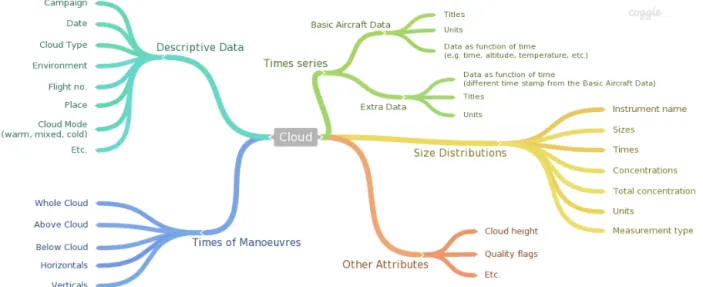
As discussed earlier, in order to use SAMAC as a comparison platform for different clouds with wide ranging characteris-tics, we need a standard but flexible data structure that can accommodate many situations. In this section, the structure of the cloud object, ways to add to the structure, as well as current methods and functions associated to cloud objects are discussed. The current overall structure of a cloud object is described in Fig. 3.
The structure’s core section is the “Basic Aircraft Data”. This section includes the time series from all instruments sharing the same time stamp as the aircraft data (with ex-ception of the size distributions). The Basic Aircraft Data section could contain, for example, time, altitude, latitude, longitude, and other quantities that happen to share the same time stamp. Titles and units of the data are also stored in the structure so that it is possible to scan the data for spe-cific quantities and keep track of the units. The methods and functions are programmed to recognize a number of titles and units combinations when looking for certain quantities. If users have data that do not share the same time stamp as the Basic Aircraft Data, these data can either be interpolated to a common time stamp or be placed in a section called “Ex-tradata”. When the data needed are not found in the Basic Aircraft Data section, the software scans the Extradata sec-tion for that data, and uses it if found. If the same data title is found in both sections, the data found in the Basic Aircraft Data is used.
Another important section is the “Size Distribution” sec-tion. This section is designed especially to handle size dis-tribution formats and representations, and is separate from the Basic Aircraft Data section. It stores the aerosol, droplet, or drizzle concentrations as a function of time and size. The time and the average particle sizes are placed in their own vectors, similarly to the total concentration, mean diameter and median diameter. Each size distribution has a record of the instrument’s name or distribution’s name, the concentra-tion’s units and the distribution type (aerosol, cloud droplet, etc.).
It may be a good idea to save the names and paths of the original files from which the data originated in the cloud in-stance itself. The structure is flexible enough to accommo-date the addition of such information without affecting the methods and functions.
The “Times of Manoeuvres” section keeps track of the times when the aircraft is executing certain manoeuvres in relation to the cloud. These times are determined by the user who can use the graphical interface to visualize the cloud and
Figure 3.Basic structure of the cloud object. All main sections are created upon initialization of a cloud instance (except for the Descriptive Data section, which is created using the method describe).
aircraft position and click on the start and end time. In this section, the beginning and end time of each manoeuvre is stored as follows: the aircraft being in the area of the cloud (as opposed to being on its way to or from the airport), being above-, below-, horizontally in-cloud, and vertical profiles. Because only the start and end times are stored, two manoeu-vre types can take place at the same time and be treated as separate manoeuvres without having to keep two copies of the same data. For example, the last few seconds of a verti-cal manoeuvre can also belong to the beginning of an above cloud manoeuvre. Because of this section, it is easy to isolate a particular manoeuvre to make a calculation, such as calcu-lating the average aerosol size distribution below-cloud only. This section can be populated manually or using a graphical interface and clicking at the beginning and end time of each manoeuvre.
The “Descriptive Data” section is where all the keywords relevant to data analysis are stored. Such descriptive key-words include the name of the measurement campaign or project, the type of cloud, the cloud’s environment, the place where the cloud is situated, etc. This allows for automatically searching and selecting only the relevant cloud instances for a given analysis project. There is a method that allows users to populate and create new characteristics in this section.
Finally, the “Other Attributes” section contains attributes of the cloud instance that cannot be calculated without hu-man intervention. Because huhu-man intervention requires time, these attributes are stored in this section to be retrieved when-ever needed. This can, for example, include quality flags or classification results. The data found in this section needs to be reviewed when a change to the original data is made.
Other main sections like the ones described here can be added to a cloud object. It can be added locally, only for the user, by adding a section to a cloud instance, or globally by
adding a section to be created upon initialization of a new cloud object (recommended). This can be done by modifying the __init__function in the “Class” file (Cloud.py).
After creating cloud instances by populating the struc-ture, it is recommended to store the cloud instances in a list of instances and to save that list of cloud instances or cloud database. Users can then load the database and mod-ify the data further or start the analysis of the data set. It is also possible to scan the cloud database for a selection of clouds (based on some criteria) and compare them easily (see Sect. 5.2 for illustration).
4.2 Methods and functions in SAMAC
Flexibility and the possibility to add new sections or new data types to the structure is accommodated: a user can cre-ate a new section at any point without disturbing the built-in methods and functions, as long as the existing sections of the structure are not affected by the modifications. Once the data is in place in a cloud object, methods and functions (rou-tines or algorithms) can be applied. SAMAC is also flexible regarding functions: users can easily add new functions with-out disturbing the existing ones.
Some of the routines available provide output (such as calculation functions), and others do not (such as object-modifying methods). In the case of SAMAC, these modi-fying methods are used to add new data or filter data that were downloaded from the source files. We try to avoid delet-ing or modifydelet-ing permanently any of the original data us-ing methods to prevent accidental changes from takus-ing place. The users are, however, still capable of modifying the orig-inal data by directly manipulating the cloud instance’s data. There is also a method meant to filter erroneous or dummy data using NumPy’s masked arrays. By using masked arrays,
the erroneous data is masked (and thus not used in calcula-tions or plots) yet the data is still stored and can be retrieved if needed.
The existing output functions in SAMAC are mostly de-signed to generate standard plots (e.g. profile plots) and re-turn calculated quantities (e.g. average amount of drizzle drops). The advantage with functions returning calculations compared to calculating a quantity once and storing it, is that the quantity is automatically updated if the original data is modified (e.g. if it underwent a re-calibration). The next time a user will access the calculated quantity, its value will be the latest one. Through this procedure, there is virtually no risk to forget to update the value because it is calculated every time it is accessed.
SAMAC does not include any data pre-processing algo-rithms i.e. instrument-specific corrections applied to raw data (e.g. Bond et al., 1998; Anderson and Ogren, 1998; Virkkula, 2010 and Wiedensohler et al., 2012). Such a pre-processing software for airborne measurements already exists, for ex-ample, EGADS (EUFAR General Airborne Data-processing Software). There are already efforts to harmonize these processes, notably through the Workshop on Data Analy-sis of Cloud Microphysical Measurements (interested read-ers may contact the organizer, Darrel Baumgardner, at [email protected]). The implementation of such algorithms to SAMAC is out of the scope of this paper but users are very welcome to add them to SAMAC if they so wish.
5 Software use
5.1 Basic use of Python commands with SAMAC
In this section, we give example lines of code to create a cloud instance and use it. Some samples of code we used to create our own cloud instances from a data file are available in the download package and the wiki pages. SAMAC has so far been used with IPython and with IPython Notebook, interactive shells for Python. We therefore recommend that users install IPython/Notebook to run the software, so better support can be provided.
The first step for using SAMAC is to create a cloud in-stance. For example,
import Cloud
MyFirstCloud=Cloud.Cloud(data, title,units,times,sizedists)
where data, title, units, times, and sizedists are input vari-ables containing the cloud’s data in the specified cloud ob-ject format, available in the wiki pages. The first line im-ports the cloud class or cloud object, and the second line cre-ates a cloud instance called “MyFirstCloud”. Explanations as to how to generate an empty cloud instance are available on the wiki pages under Initialization. These cloud instances must be saved so they can be loaded (and further modified if needed) in a later session. The authors have been
suc-cessfully saving/compressing their instances using the pickle module on a single list of cloud instances that we call a cloud database. Note that other compression methods than pickle may also be suitable for SAMAC Cloud objects.
There are several ways to create a cloud instance. All involve the command lines above, but the way the data is put into it can vary. Along with SAMAC, we provide our own code that guides the user into finding the relevant data, shaping the data, and creating the cloud. This piece of code is tailored for our own data formats and modifi-cations will very likely be necessary. Another, and perhaps simpler, way would be to prepare the data, title, units, times and sizedists variables into the specified formats and use the “Cloud.Cloud” command passing those variables as input. Yet another way to create an instance would be to create an empty cloud instance, and populate it manually afterwards. It is also possible to use a mix of passing the data directly and populating it afterwards. Post-populating the cloud can be done using some of the built-in methods, especially the methods timechange in the case of the variable times, addsdfor the variable sizedists, and add2basic for vari-ables data, title, and units.
The data in the cloud object can be accessed using the name of the cloud and its address. For example, the manoeu-vre times are accessed like this:
MyFirstCloud.times
To calculate the average value of the total concentration of the first size distribution in the list of distributions, the ad-dress of the data is used as if it were a variable:
Average_value=numpy.mean
(MyFirstCloud.sd[0][‘‘total”])
where numpy.mean is an averaging function available in the NumPy extension, and MyFirstCloud.sd[0][“total”] is the address of the total concentration array for the first (indicated by 0, because python uses zero-based numbering) size distri-bution.
Methods must always be called with parentheses after their name. For example, to create or modify a cloud’s description section, a user would type the following:
MyFirstCloud.describe()
and then create or modify the section through questions in the prompt. If input variables are required, these variables are defined inside the parentheses. Functions always include the cloud instance in their call, and they may also include in-put variables or options other than the cloud instance. They are added after the cloud instance. For example, the function plotavsdplots the average size distribution for a given manoeuvre and instrument. The function that generates this plot must then be called like this:
samac.plotavsd(MyFirstCloud,prof= ’verticloud’,scan=2,inst=’FSSP’)
to get the average size distribution of the 3rd (indicated with scan=2, because of zero-based numbering) vertical profile (verticloud), for the instrument called FSSP (Forward Scat-tering Spectrometer Probe).
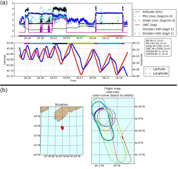
Figure 4.Panel (a) shows a qualitative view of the aircraft’s altitude, the measured particle and cloud droplet total concentrations, the liquid water content and drizzle drop concentration in its upper subplot, and the aircraft’s latitude and longitude on the lower subplot. All the data in the upper subplot can be magnified and/or offset (values of which are indicated in the rounded box on the right-hand side of the plot). At its bottom, a colour-coded time tracker is inserted. The lower subplot shows the latitude (left axis) and longitude (right axis) of the aircraft or probe. At its top, the colours indicate which manoeuvre the aircraft is making (magenta = vertical, cyan = below cloud, black = horizontal in cloud and yellow = above cloud). Panel (b) shows the path of the aircraft or probe while the cloud instance was being measured. The subplot on the left shows a zoomed-out map and the subplot on the right shows a zoomed-in situation, with the size of the points corresponding to the liquid water content and the colour corresponding to the time tracker in the time series (Panel (a)).
In the case where input variables are required but default values are already defined in the function, the user can choose to define those variables (and change them) or not. For ex-ample, the default for plotavsd is already defined in the function and is prof=’belowcloud’, num=0, inst=’PCASP’. If a user wants to see the average size distribution for the first below-cloud manoeuvre from the PCASP (Passive Cav-ity Aerosol Spectrometer Probe), it would be enough to type this line:
samac.plotavsd(MyFirstCloud)
but this line would give the same result because these options are the default options:
samac.plotavsd(MyFirstCloud,prof= ’belowcloud’,num=0,inst=’PCASP’)
Input variable definitions and default inputs are explained in the help section of each method and function. To read the description for function plotavsd, a user can request help using this line:
help(samac.plotavsd)
and this line to read the description for method addsd: help(MyFirstCloud.addsd)
Figure 5. Two functions that display the vertical profile of a cloud. In this cloud instance, the aircraft made three vertical profiles (in addition to two below-cloud manoeuvres, two above-cloud manoeuvres and one in-cloud horizontal manoeuvre). Panel (a) was created using the function wholeprof and displays the liquid water content, FSSP total concentrations, PCASP total concentration, relative humidity, drizzle concentrations above 100 and 200 microns, as well as temperature and theta Q for all the manoeuvres as a function of altitude on the yaxis. Panel (b) was created using the function vprof and displays the same quantities as (a) as well as the effective radii of the FSSP and PCASP for the first vertical profile only, as a function of altitude on the y axis.
5.2 Example use from the Canadian SOLAS 2003 campaign
The first measurement campaign on which the software was tested was the Canadian SOLAS 2003 campaign (Leaitch et al., 2010). In this section, we will use examples from that campaign to illustrate how SAMAC can be used for scien-tific research. In this version of the software, methods and functions as well as the structure were designed to study the aerosol–cloud–precipitation interaction, but we would like to emphasize that it would cost little effort to add sections to the structure or add methods and functions to fit other types of studies while using SAMAC’s reproducibility and compara-bility advantages.
In this section, we illustrate how SAMAC can be used for research using a very simple example: we want to verify how the amount of drizzle varies with varying LWP (liquid water path) for clouds that were measured during SOLAS 2003. We first need to place the measured data in the cloud structure, as shown in the wiki pages.
After placing the original data into the SAMAC cloud structure, we generated an overview of the results us-ing the functions overview and mapcloud respectively (Fig. 4). Using the colour-coded time tracker, we used method timechange to click at the beginning and end of each leg (below-cloud, above-cloud, vertically in-cloud, hor-izontally in-cloud). We used the method describe to en-ter general information on the cloud using existing keys and adding new ones. We also used MaskData to filter unphys-ical or erroneous data points (Fig. 2). We then used methods defheightand defBGheight to define the cloud base and cloud top by simply clicking on vertical profile plots (Fig. 5). Finally, we used lwcflag to evaluate the quality of the liquid water content profiles for every vertical profile.
We designed a new calculation function to calculate the total amount of drizzle in vertical profiles that we called totalvolprecip and saved it in a file identifying the authors (with “Dal” in its name). With function contribu-tions from other researchers, we could compare our respec-tive functions and investigate differences in the results.
Using the functions and methods currently available in SAMAC 1.0.0, we were able to easily plot an indicator of precipitation as a function of the liquid water path for all ver-tical profiles of stratiform, marine clouds using only a few lines of code. With all the measured clouds in a list of clouds called CloudList, these few lines generated Fig. 6.
1 index=[i for i,c in enumerate (CloudList) if c.desc["cloudtype"] =="stratiform" and c.desc
["environment"]=="maritime"] # selects stratiform maritime clouds Precip=list();
2 LWPs=list(); # initializes lists 3 for i in index: # for each cloud 4 for j in range(len(CloudList[i].
Figure 6.Figure resulting from the example code at the end of Sect. 5.2. Here, we plotted an indicator of the drizzle volume in a vertical profile as a function of the liquid water path. This is only an example; many other possibilities exist.
times["verticloud"])): # for each vertical leg
5 Precip.append(samac.totalvolprecip (CloudList[i], abovesize=100, scan=j,filler=0))
# uses totalvolprecip to calculate an indicator of precipitation and add it to the list Precip
6 LWPs.append(samac.lwp
(CloudList[i])[j][0]) # uses lwp to get the LWP and add
it to the list LWP
7 semilogy(LWPs,Precip,’bo’) # plots the results
8 xlabel(’Liquid Water Path (g m$ˆ{-2}$)’)
9 ylabel(’Total volumic precipitation (a.u.)’)
Note that the numbers at the beginning of the lines are to indicate line number and are not part of the code. Plotting of complex quantities is simplified by the use of methods and functions, and the list of clouds can easily be scanned for cloud instances with selected characteristics.
6 Conclusions
We present a new software package, SAMAC, available at https://github.com/StephGagne/SAMAC and designed for the analysis of cloud measurement data using the program-ming language Python 2.7. The use of SAMAC by the aerosol–cloud–precipitation research community can speed-up the analysis of cloud data and facilitate comparisons among data sets and within and among research groups.
Through the release of this software as an open-source project, the quality of the software will improved because of its evaluation by other researchers, and the existing func-tions and the diversity of funcfunc-tions will improve because of users coding according to their needs and submitting their new functions. Moreover, by sharing this software, all users save on coding time by distributing the work load. We illus-trated how the use of the basic features of SAMAC could be useful for research, and believe it would be particularly useful when comparing algorithms.
Although we recognize the need for further improvements, at its current stage, SAMAC is advanced enough for other groups to profit from its use. Reciprocally, SAMAC will ben-efit from a larger base of users with different needs, capable of contributing to the software. Contribution to the software should cost little effort other than harmonizing the user’s code to the existing code and will centralize aerosol–cloud– precipitation measurement handling, and make results more comparable to other users’ results, thus providing more con-sistent results to modellers. In the context of a call for pub-lishing data analysis code with scientific articles to improve traceability and reproducibility, we believe that SAMAC would be a great platform around which the cloud measure-ment community could gather and share parts of their data analysis code.
Acknowledgements. The authors would like to thank David Delene from University of North Dakota for his constructive comments on an early version of this software and for his sustained interest in this project. NSERC’s Visiting Fellowships in Canadian Government Laboratories Program is acknowledged for Stéphanie Gagné’s funding. The NSERC USRA program is acknowledged for Landan MacDonald’s funding.
Edited by: P. Herckes
References
Anderson, T. L. and Ogren, J. A.: Determining Aerosol Radia-tive Properties Using the TSI 3563 Integrating Nephelometer, Aerosol Sci. Tech. 29, 57–69, doi:10.1080/02786829808965551, 1998.
Atmospheric Science Software Applications – UCAR Commu-nity Tools (2009): available at: https://www.ucar.edu/tools/ applications_desc.jsp (last access: 1 January 2016), 2009. Barnes, N.: Publish your computer code: it is good enough, Nature,
467, p. 753, 2010.
Beazley, D. M.: Python Essential Reference, 4th Ed., Developper’s Library, Addison-Wesley, Boston, USA, 2009.
Bond, T. C., Charlson, R. J., and Heintzenberg, J.: Qunatifying the emission of light-absorbing particles: Measurements tailored to climate studies, Geophys. Res. Lett., 25, 337–340, 1998. Boucher, O. and Lohmann, U.: The sulfate-CCN-cloud albedo
ef-fect: A sensitivity study with two general circulation models, Tel-lus B, 47, 281–300, 1995.
Challet, D. and Le Du, Y.: Microscopic Model of Software Bug Dy-namics: Closed Source Versus Open Source, International Jour-nal of Reliability, Quality and Safety Engineering, 12, 521–534, 2005.
Delene, D. J.: Airborne data processing and analysis software pack-age, Earth Science Informatics, 4, 29–44, 2010.
Easterbrook, S. M.: Open code for open science?, Nat. Geosci., 779–781, 2004.
EUFAR-EGADS: available at: https://code.google.com/p/ eufar-egads/, last access: 1 January 2016.
Gagné, S., MacDonald, L., et al.: Effect of the aerosol size distri-bution on clouds and precipitation – results from the Canadian SOLAS 2003 aircraft campaign, in preparation, 2016.
GitHub Help: available at: https://help.github.com/, last access: 1 February 2016.
Hunter, J. D.: Matplotlib: A 2D graphics environment, IEEE Com-puter Society, 9, 90–95, 2007.
IPCC: Climate Change 2007: The Physical Science Basis, Contri-bution of Working Group I to the Fourth Assessment Report of IPCC, edited by: Solomon, S., Qin, D., Manning, M., Chen, Z., Marquis, M., Averyt, K. B., Tignor, M., and Miller, H. L., Cam-bridge University Press, CamCam-bridge, UK and New York, NY, USA, 996 pp., 2007.
Johnson, D. W., Osborne, S., Wood, R., Suhre, K., Johnson, R., Businger, S., Quinn, P. K., Wiedensohler, A., Durkee, P. A., Rus-sell, L. M., Andreae, M. O., O’Dowd, C., Noone, K. J., Bandy, B., Rudolph, J., and Rapsomanikis, S.: An overview of the La-grangian experiments undertaken during the North Atlantic re-gional Aerosol Characterisation Experiment (ACE-2), Tellus, 52B, 290–320, 2000.
Kleinman, L. I., Daum, P. H., Lee, Y.-N., Lewis, E. R., Sedlacek III, A. J., Senum, G. I., Springston, S. R., Wang, J., Hubbe, J., Jayne, J., Min, Q., Yum, S. S., and Allen, G.: Aerosol concentration and size distribution measured below, in, and above cloud from the DOE G-1 during VOCALS-REx, Atmos. Chem. Phys., 12, 207– 223, doi:10.5194/acp-12-207-2012, 2012.
Leaitch, W. R., Banic, C. M., Isaac, G. A., Couture, M. D., Liu, P. S. K., Gultepe, I., Li, S.-M., Kleinman, L., Daum, P. H., and MacPherson, J. I.: Physical and chemical observations in ma-rine stratus during the 1993 North Atlantic Regional Experiment: Factors controlling cloud droplet number concentrations, J. Geo-phys. Res., 101, 29123–29135, 1996.
Leaitch, W. R., Lohmann, U., Russell, L. M., Garrett, T., Shantz, N. C., Toom-Sauntry, D., Strapp, J. W., Hayden, K. L., Marshall, J., Wolde, M., Worsnop, D. R., and Jayne, J. T.: Cloud albedo increase from carbonaceous aerosol, Atmos. Chem. Phys., 10, 7669–7684, doi:10.5194/acp-10-7669-2010, 2010.
Lin, J. W.-B.: Why Python is the next wave in Earth Sci-ences Computing, B. Am. Meteorol. Soc., 93, 1823–1824, doi:10.1175/BAMS-D-12-00148.1, 2012.
Lu, M.-L., Conant, W. C., Jonsson, H. H., Varutbangkul, V., Flagan, R. C., and Seinfeld, J. H.: The Marine Stra-tus/Stratocumulus Experiment (MASE): Aerosol-cloud relation-ships in marine stratocumulus, J. Geophys. Res., 112, D10209, doi:10.1029/2006JD007985, 2007.
Masked Arrays – NumPy v1.8 Manual: availabe at: http://docs. scipy.org/doc/numpy/reference/maskedarray.html, last access: 1 December 2013.
Matplotlib Python Plotting – Matplotlib 1.3.1 documentation: avail-able at: http://matplotlib.org/, last access: 1 February 2016. Merali, Z.: Why scientific programming does not compute, Nature,
467, 775–777, 2010.
Morrison, H., Curry, J. A., and Khvorostyanov, V. I.: A new double-moment microphysics parameterization for application in cloud and climate models. Part I: Description, J. Atmos. Sci., 62, 1665– 1677, 2005.
Nature Editorial: Journals unite for reproducibility, Nature, 515, p. 7, 2014.
Nenes, A. and Seinfeld, J. H.: Parameterization of cloud droplet formation in global climate models, J. Geophys. Res., 108, 4415, doi:10.1029/2002JD002911, 2003.
NumPy: available at: http://www.numpy.org/, last access: 1 Decem-ber 2013.
Perkel, J. M.: Programming: Pick up Python, Nature, 518, 125–126, 2015.
Python Programming Language – Official Website: www.python. org, last access: December 2013.
Rauber, R. M., Zhao, G., Di Girolamo, L., and Colón-Robles, M.: Aerosol size distribution, particle concentration, and optical property variability near Caribbean trade cumulus clouds: Iso-lating effects of vertical tranport and cloud processing from hu-midification using aircraft measurements, J. Atm. Sci., 70, 3063– 3083, doi:10.1175/JAS-D-12-0105.1, 2013.
RPy: A simple and efficient access to R from Python: available at: http://rpy.sourceforge.net/, last access: December 2013. Schmid, B., Livingston, J. M., Russell, P. B., Durkee, P. A., Jonsson,
H. H., Collins, D. R., Flagan, R. C., Seinfeld, J. H., Gassó, S., Hegg, D. A., Öström, E., Noone, K. J., Welton, E. J., Voss, K. J., Gordon, H. R., Formenti, P., and Andreae, M. O.: Clear-sky clo-sure studies of lower tropospheric aerosol and water vapor dur-ing ACE-2 usdur-ing airborne sunphotometer, airborne in-situ, space-borne, and ground-based measurements, Tellus, 52B, 568–593, 2000.
SciPy.org – SciPy.org: available at: http://www.scipy.org/, last ac-cess: December 2013.
Sollazzo, M. J., Russell, L. M., Percival, D., Osborne, S., Wood, R., and Johnson, D. W.: Entrainment rates during ACE-2 Lagrangian experiments calculated from aircraft measurements, Tellus, 52B, 335–347, 2000.
Unidata | IDV: available at: https://www.unidata.ucar.edu/software/ idv, doi:10.5065/D6RN35XM, last access: 1 January 2016. Virkkula, A.: Correction of the Calibration of the 3-wavelength
Par-ticle Soot Absorption Photometer (3l PSAP), Aerosol Sci. Tech., 44, 706–712, doi:10.1080/02786826.2010.482110, 2010. Wiedensohler, A., Birmili, W., Nowak, A., Sonntag, A., Weinhold,
K., Merkel, M., Wehner, B., Tuch, T., Pfeifer, S., Fiebig, M., Fjäraa, A. M., Asmi, E., Sellegri, K., Depuy, R., Venzac, H., Vil-lani, P., Laj, P., Aalto, P., Ogren, J. A., Swietlicki, E., Williams, P., Roldin, P., Quincey, P., Hüglin, C., Fierz-Schmidhauser, R., Gysel, M., Weingartner, E., Riccobono, F., Santos, S., Grüning, C., Faloon, K., Beddows, D., Harrison, R., Monahan, C., Jen-nings, S. G., O’Dowd, C. D., Marinoni, A., Horn, H.-G., Keck, L., Jiang, J., Scheckman, J., McMurry, P. H., Deng, Z., Zhao, C. S., Moerman, M., Henzing, B., de Leeuw, G., Löschau, G., and Bastian, S.: Mobility particle size spectrometers: harmonization of technical standards and data structure to facilitate high qual-ity long-term observations of atmospheric particle number size distributions, Atmos. Meas. Tech., 5, 657–685, doi:10.5194/amt-5-657-2012, 2012.
Wood, R., Mechoso, C. R., Bretherton, C. S., Weller, R. A., Huebert, B., Straneo, F., Albrecht, B. A., Coe, H., Allen, G., Vaughan, G., Daum, P., Fairall, C., Chand, D., Gallardo Klenner, L., Garreaud, R., Grados, C., Covert, D. S., Bates, T. S., Krejci, R., Russell, L. M., de Szoeke, S., Brewer, A., Yuter, S. E., Springston, S. R., Chaigneau, A., Toniazzo, T., Minnis, P., Palikonda, R., Abel, S. J., Brown, W. O. J., Williams, S., Fochesatto, J., Brioude, J., and Bower, K. N.: The VAMOS Ocean-Cloud-Atmosphere-Land Study Regional Experiment (VOCALS-REx): goals, plat-forms, and field operations, Atmos. Chem. Phys., 11, 627–654, doi:10.5194/acp-11-627-2011, 2011.
Yarkoni, T.: The homogenization of scientific computing, or why Python is steadily eating other languages’ lunch: available at: http://www.r-bloggers.com/the-homogenization-of-scientific- computing-or-why-python-is-steadily-eating-other-languages-lunch/, last access: 2 December 2013.
Zhang, K., Liu, X., Wang, M., Comstock, J. M., Mitchell, D. L., Mishra, S., and Mace, G. G.: Evaluating and constraining ice cloud parameterizations in CAM5 using aircraft measure-ments from the SPARTICUS campaign, Atmos. Chem. Phys., 13, 4963–4982, doi:10.5194/acp-13-4963-2013, 2013.