Beyond predictive modeling : new computational aspects for deep learning based biological applications

Beyond Predictive Modeling: New Computational

Aspects for Deep Learning Based Biological

Applications

by

Ge Liu

B.Eng., Tsinghua University, 2015

M.S. in Electrical Engineering and Computer Science

Massachusetts Institute of Technology, 2018

Submitted to the Department of Electrical Engineering and Computer

Science

in partial fulfillment of the requirements for the degree of

Doctor of Philosophy

at the

MASSACHUSETTS INSTITUTE OF TECHNOLOGY

September 2020

c

Massachusetts Institute of Technology 2020. All rights reserved.

Author . . . .

Department of Electrical Engineering and Computer Science

August 25, 2020

Certified by . . . .

David Gifford

Professor of Electrical Engineering and Computer Science

Thesis Supervisor

Accepted by . . . .

Leslie A. Kolodziejski

Professor of Electrical Engineering and Computer Science

Chair, Department Committee on Graduate Students

Beyond Predictive Modeling: New Computational Aspects

for Deep Learning Based Biological Applications

by

Ge Liu

Submitted to the Department of Electrical Engineering and Computer Science on August 25, 2020, in partial fulfillment of the

requirements for the degree of Doctor of Philosophy

Abstract

Next generation sequencing and large-scale synthetic DNA synthesis have enabled advances in biological studies by providing high-throughput data that can efficiently train machine learning models. Deep learning models have proven to provide state-of-the-art performance for predictive tasks across many biological applications. However, black-box predictive modeling is not sufficient for scientific discovery in biology. For discovery it is important to find the mechanisms that underlie outcomes. Mecha-nism discovery requires the visualization and interpretation of black-box predictive models. Discovery further requires analyzing data from exploratory experiments, and such experiments may produce data that is dissimilar from previous observations and thus be outside of a model’s training distribution. Recognizing and quantifying the uncertainty of model predictions on out-of-distribution data is crucial for proper experiment interpretation. Moreover, therapeutic molecular design usually involves iterations of proposing and testing new candidates, which require sequential decision making and directed optimization of molecules in a multiplexed fashion. Finally, certain machine learning design tasks such as vaccine design need to meet objec-tives such as population coverage which require efficient algorithms for combinatorial optimization.

This thesis investigates and proposes novel techniques in four areas: model in-terpretation, model uncertainty, generating optimized antibody candidates, and op-timization of vaccines with population coverage objectives. We first present Deep-Resolve, a novel analysis framework for deep convolutional models of genome func-tion that visualizes how input features contribute individually and combinatorially to network decisions. Unlike other methods, DeepResolve does not depend upon the analysis of a predefined set of inputs. Rather, it uses gradient ascent to stochastically explore intermediate feature maps to 1) discover important features, 2) visualize their contribution and interaction patterns, and 3) analyze feature sharing across tasks that suggests shared biological mechanism. Next, we introduce Maximize Overall Diversity (MOD), an approach to improve ensemble-based uncertainty estimates by encouraging larger overall diversity in deep ensemble predictions across all possible

inputs. We also explore variations of MOD utilizing adversarial techniques (MOD-Adv) and data density estimation (MOD-R). We show that for out-of-distribution test examples, MOD improves predictive performance and uncertainty calibration on multiple regression and Bayesian Optimization tasks. Thirdly, we use ensembles of deep learning models and gradient based optimization in antibody sequence design. We optimize antibodies for optimized binding affinity and specificity, and experi-mentally confirm our optimization results. Last, we combine deep learning models for predicting peptide MHC display with population frequency objectives to create a novel vaccine design tool, OptiVax, that estimates and optimizes the population coverage of peptide vaccines to facilitate robust immune responses. We used OptiVax to design peptide vaccines for SARS-CoV-2 and achieved superior predicted popula-tion coverage when compared to 29 public baseline designs. Collectively our studies will enable the application of deep learning in broad range of scenarios in biological studies.

Thesis Supervisor: David Gifford

Acknowledgments

I would like to say thank you to all the mentors, labmates, and friends who made my Ph.D. an unforgettable experience in my life.

First, I want to thank my Ph.D. advisor David Gifford for his great mentorship and guidance during my Ph.D. years. I have always been inspired by Dave’s innovative vision and deep insights about science and technologies, and he has always been my role model to follow in academia. Dave taught me the most rigorous way of doing science and he is always patient and helpful. There have been so many times that I have been cheered up by Dave’s encouraging words and great sense of humor. It has been such a joyful experience working with Dave in my PhD.

I want to thank my thesis committee members Michael Birnbaum and Tommi

Jakkola for their constructive feedback on the thesis. I am also grateful for my

academic advisor Manolis Kellis for providing insightful advice on my course selection and career development.

I thank all members of the Gifford lab for being such great lab-mates and making my PhD life delightful. I especially thank Haoyang Zeng for his help and guidance in my early PhD years, and it has been a pleasure collaborating with him on research. I thank Sid Jain for being such a great collaborator and for offering helpful advises to my research and life. I thank Jonas Mueller, Brandon Carter and Ziheng Wang for the insightful discussions and productive collaborations, Grace Yeo for the hard work maintaining lab clusters.

I am also grateful to my collaborators at Novartis Biomedical Research, Stefan Ewert for offering the precious opportunity to cooperate on the antibody project and being such a responsible and productive lead on the experimental side, Jonas Schilz and Geraldine Horny for the effort in conducting the wet lab experiments. I thank Richard Sherwood for the helpful advises and Brooke Huisman for the insightful discussions.

Lastly, I want to say thank you for the companionship and support from my friends and family. Thank you mom and aunt for the unconditional love you offer that has been my power to advance in my oversea graduate school life.

Contents

1 Introduction 23

1.1 Motivation . . . 23

1.2 Thesis Structure . . . 25

1.3 Prior publication . . . 25

2 Visualizing Complex Feature Interactions and Feature Sharing in Genomic Deep Neural Networks 27 2.1 Introduction . . . 27

2.2 Methods . . . 30

2.2.1 Visualizing feature importance and combinatorial interactions 30 2.2.2 Visualizing feature sharing and class relationship . . . 33

2.2.3 Implementation details . . . 34

2.3 Results . . . 35

2.3.1 Synthetic datasets . . . 35

2.3.2 Experimental datasets . . . 40

2.4 Discussion . . . 48

2.4.1 Potential artifacts in minor cases . . . 48

2.4.2 Intermediate layer selection for analysis . . . 50

2.4.3 Selection of hyper-parameters . . . 50

2.4.4 Complex logic and feature sharing in biological problems . . . 51

2.4.5 Combining DeepResolve with existing tools . . . 51

3 Maximizing Overall Diversity for Improved Uncertainty Estimates in Deep Ensembles 53 3.1 Introduction . . . 53

3.2 Related Work . . . 54

3.3 Methods . . . 55

3.3.1 Maximizing Overall Diversity (MOD) . . . 56

3.3.2 Maximizing Reweighted Diversity (MOD-R) . . . 58

3.3.3 Maximizing Overall Diversity with Adversarial Optimization (MOD-Adv) . . . 59

3.4 Results . . . 60

3.4.1 Baseline Methods . . . 60

3.4.2 Experiment Details . . . 61

3.4.3 Univariate Regression . . . 61

3.4.4 Protein Binding Microarray Data . . . 62

3.4.5 UCI Regression Datasets . . . 66

3.4.6 Age Prediction from Images . . . 68

3.5 Conclusion . . . 68

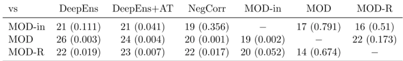
4 Deep Learning Based Antibody Complementarity Determining Re-gion Design 71 4.1 Introduction . . . 71

4.2 Antibody binding prediction with deep learning . . . 73

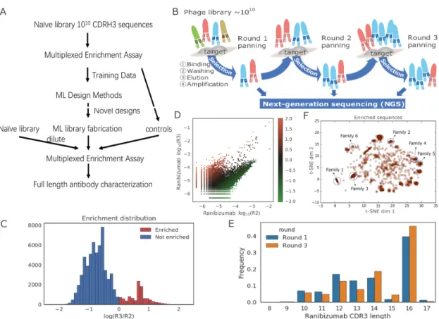
4.2.1 Phage-panning data generation . . . 73

4.2.2 Training an ensemble of neural networks to predict enrichment from antibody sequence . . . 75

4.2.3 Results . . . 75

4.3 Antibody specificity prediction and computational counter panning . 78 4.3.1 Target antigens . . . 78

4.3.2 Computational counter-panning . . . 79

4.3.3 Generalizing non-specificity prediction for new targets with sim-ilar structure . . . 83

4.4 Optimizing antibody sequences with gradient ascent and a neural net-work ensemble . . . 85

4.4.1 Ensembles and voting strategy used in sequence optimization 87

4.4.3 Machine learning designed sequences are better than panning

derived sequences . . . 91

4.5 Discussion . . . 94

4.6 Experimental material and data preparation . . . 97

4.6.1 Single framework library generation . . . 97

4.6.2 IgG expression . . . 98

4.6.3 Phage Display panning against a target molecule . . . 98

4.6.4 Next Generation Sequencing (NGS) sample preparation . . . . 99

4.6.5 Data preparation . . . 99

4.6.6 Oligo synthesis of CDR-H3 sequences and library generation . 101 4.6.7 ELISA . . . 102

4.6.8 Enforcing compositional constraints in sequences used for oligo synthesis . . . 102

4.6.9 Stringent washing improves antibody EC50 prediction . . . 103

4.6.10 Selecting experiment derived top sequences for EC50 measure-ment . . . 103

5 Population Coverage Optimization for Peptide Vaccine Design and its Application to SARS-CoV-2 Vaccine Design 105 5.1 Introduction . . . 105

5.1.1 Designing peptide vaccine that targets human haplotype distri-butions . . . 107

5.1.2 Designing peptide vaccine that ensures a diverse display of pep-tides in population (multi-coverage problem) . . . 108

5.1.3 Augmenting subunit vaccines for robust coverage . . . 109

5.2 The Maximum n-times coverage problem . . . 110

5.2.1 _{Set Cover and Maximum Coverage . . . .} 110

5.2.2 Maximum n-times Coverage . . . 111

5.2.3 _{The MarginalGreedy algorithm for maximum n-times} cov-erage . . . 114

5.2.4 MarginalGreedy outperforms a greedy baseline on toy ex-amples . . . 114

5.3 Population coverage evaluation and optimization . . . 116

5.3.1 SARS-CoV-2 proteome and candidate peptides . . . 118

5.3.2 Peptide filtering . . . 120

5.3.3 HLA population frequency computation . . . 122

5.3.4 Peptide scoring with computational peptide-HLA prediction models . . . 124

5.3.5 EvalVax population coverage evaluation tool . . . 127

5.3.6 OptiVax vaccine population coverage optimization tool . . . . 130

5.3.7 Evaluation and augmentation of subunit vaccine . . . 133

5.4 Results . . . 135

5.4.1 De novo design of peptide vaccine for SARS-CoV-2 with sepa-rate peptide sets for MHC class I and II . . . 135

5.4.2 De novo design of peptide vaccine for SARS-CoV-2 with a joint peptide set for MHC class I and II . . . 140

5.4.3 Comparison to public peptide vaccine designs for SARS-CoV-2 140 5.4.4 Evaluation of subunit vaccines . . . 144

5.4.5 Augmentation of subunit vaccines with separate peptide sets for MHC class I and II . . . 147

5.4.6 Augmentation of subunit vaccines with a single joint peptide sets for MHC class I and II . . . 149

5.4.7 Joint designs are more compact than separate designs . . . 149

6 Conclusions and Future Work 153 6.1 Uncertainty estimation . . . 154

6.2 Antibody design . . . 154

6.3 Peptide vaccine design . . . 155 A Visualizing Complex Feature Interactions and Feature Sharing in

Genomic Deep Neural Networks 157

B Deep Learning Based Antibody Complementarity Determining

C Population Coverage Optimization for Peptide Vaccine Design and

List of Figures

2-1 Illustration of DeepResolve’s working flow. . . 32

2-2 Illustration of the generation of OFIV from FIVs generated by all 10

runs of gradient ascent in synthetic data set I. . . 36 2-3 Distribution of optimal number of Gaussian mixture component of

vari-ances in each set of experiments. . . 37

2-4 Input-dependent visualizations produce unstable results on XOR logic

and fail to capture the XOR interaction. . . 38

2-5 Visualization of DeepResolve in multi-task networks. . . 39

2-6 Distribution of positive sample activation level, negative sample ac-tivation level and motif matching p-values of filters grouped by their ONIV score ranking. . . 42 2-7 Visualization of sequence features captured by the 480 channels in 2nd

convolutional layer of DeepSEA. . . 43

2-8 Class similarity map for DeepSEA’s output classes including 919

dif-ferent experiments including DNase I hypersensitivity, TF binding and histone marks across different cell types. . . 45

2-9 Bi-clustering of TF/histone mark - DNase hypersensitivity similarity

map(A) and bar-plot of number of strong positive (red) and strong negative class similarity (blue) with DNase experiments for each of the TFs and histone marks (B). . . 46 2-10 Hierarchical clustering results of 919 biological targets using correlation

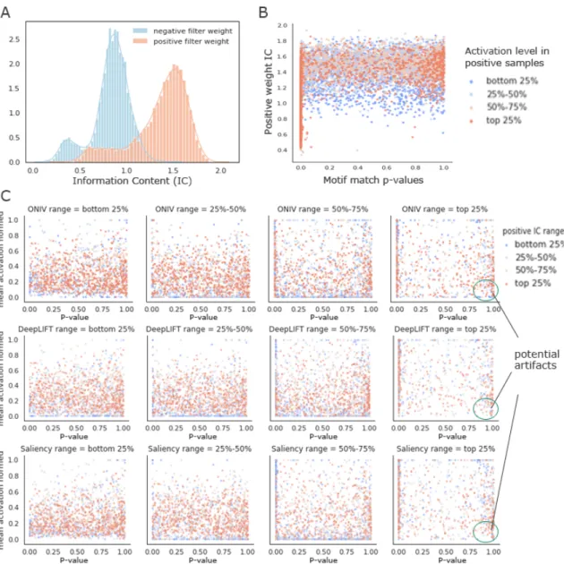
2-11 Distribution of information content of positive and negative weights in all filters in the 422 TF binding models (A).Positive weight informa-tion content verses the TOMTOM p-value with known motif for all convolutional filters colored by the activation level in positive exam-ples (B).Positive sample activation verses motif matching p-values for filters grouped by their attribution scores (C). . . 49

3-1 Regression on synthesized data with 95% confidence intervals (CI). . 55

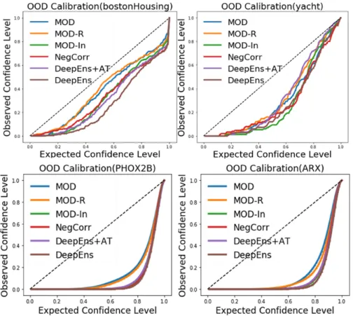
3-2 Calibration curves for regression models trained on two of the UCI

datasets (top) and two DNA TF binding datasets (bottom). . . 64

3-3 Regret for two Bayesian optimization tasks (averaged over 20 replicate runs). . . 65

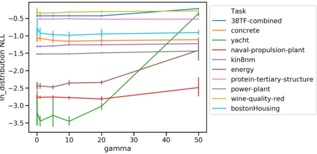
3-4 The effect of different γ on in-distribution test performance (NLL). . 67

4-1 Summary of the training data used in our machine learning framework. 74

4-2 Performance of our neural networks in predicting ranibizumab

enrich-ment. . . 76

4-3 Convolutional neural networks can accurately extrapolate to new

se-quences which are more positively enriched than the entirety of the training set. . . 77 4-4 Machine learning classification of antibody specificity. . . 80

4-5 Computational counter-panning removes off-target binders more

effec-tively than molecular counter-panning. . . 81

4-6 Computational counter-panning has a lower false positive and false

negative rate than molecular counter-panning. . . 81

4-7 Computational counter-panning produces superior classifications for

48 selected sequences using Fab/IgG and cross-panning / on-target panning ratios. . . 83 4-8 Computational counter panning provides superior classifications using

ground truth metrics from Octet/ELISA data for 48 candidates. . . . 84

4-9 Machine learning can reject undesired antibodies. . . 85

4-11 Overview of the alternative VAE approach to produce high-affinity sequences. . . 90 4-12 Experimental results of the ML-proposed library diluted 1:100 into our

initial synthetic library. . . 92

4-13 Additional experimental result on Ens-Grad proposed sequence. . . . 93

4-14 Visualization of machine learning (ML) optimization. . . 95

5-1 Example of n-times coverage calculation. . . 113

5-2 _{The MarginalGreedy algorithm outperforms the greedy algorithm}

on toy examples. Superior performance is seen on both the n-times Set Cover and Maximum n-times Coverage problems. Shaded regions indicate 95% confidence intervals. . . 116

5-3 _{The MarginalGreedy algorithm outperforms the greedy algorithm}

and approaches true optimal on toy examples. Superior performance is seen on both the n-times Set Cover and Maximum n-times Coverage problems. Shaded regions indicate 95% confidence intervals.116

5-4 Overview of the OptiVax and EvalVax machine learning system for

combinatorial vaccine optimization and evaluation. . . 117

5-5 The separate and joint design methods for peptide vaccines. . . 118

5-6 Illustration of functional domains on SARS-CoV-2 S protein. . . 119

5-7 SARS-CoV-2 OptiVax-Robust selected peptide vaccine set for (A) MHC

class I and (B) MHC class II. (a) EvalVax-Robust population cov-erage at different per-individual number of peptide-HLA hit cutoffs for populations self-reporting as having White, Black, or Asian ances-try and average values. (b) EvalVax-Unlinked population coverage on 15 geographic regions and averaged population coverage. (c) Binding of vaccine peptides to each of the available alleles in MHC I and II. (d) Peptide viral protein origins. (e) Distribution of the number of per-individual peptide-HLA hits in populations self-reporting as hav-ing White, Black, or Asian ancestry. (f) Vaccine peptide presence in SARS-CoV. . . 136

5-8 OptiVax-Robust designed peptide vaccine using peptides from the SARS-CoV-2 S, M, and N proteins only. (A) Results for MHC class I and (B) MHC class II. (a) EvalVax-Robust population coverage at different minimum number of peptide-HLA hit cutoffs. (b) EvalVax-Unlinked population coverage. (c) Binding of vaccine peptides to each of the available alleles in MHC I and II. (d) Peptide viral protein origins. (e) Distribution of the number of per-individual peptide-HLA hits in populations self-reporting as having White, Black, or Asian ancestry. (f) Vaccine peptide presence in SARS-CoV. . . 137

5-9 OptiVax-Unlinked selected SARS-CoV-2 optimal peptide vaccine set

for (A) MHC class I and (B) MHC class II. (a) EvalVax-Robust popu-lation coverage at different per-individual number of peptide-HLA hits cutoffs for populations self-reporting as having White, Black, or Asian ancestry and average value. (b) EvalVax-Unlinked population cover-age on 15 geographic regions and avercover-aged population covercover-age. (c) Binding of vaccine peptides to each of the available alleles in MHC I and II. (d) Peptide viral protein origins. (e) Distribution of the num-ber of per-individual peptide-HLA hits in populations self-reporting as having White, Black, or Asian ancestry. (f) Vaccine peptide presence in SARS-CoV. . . 139 5-10 Predicted uncovered percentage of the population for MHC peptide

display using a joint set as a function of the number of 25-mer at different predicted peptide-HLA hit thresholds in each individual. . . 140 5-11 Predicted coverage in populations self-reporting as White, Black, and

Asian with a peptide-only vaccine comprising 24 25-mer peptides jointly optimized for MHC class I and MHC class II coverage. The red dotted vertical line shows the expected number of hits. . . 141 5-12 EvalVax population coverage evaluation, expectation of per individual

number of peptide-HLA hits and normalized coverage for MHC class I SARS-CoV-2 vaccines. . . 142

5-13 EvalVax population coverage evaluation, expectation of per individual number of peptide-HLA hits and normalized coverage for MHC class II SARS-CoV-2 vaccines. . . 143 5-14 Predicted uncovered percentage of populations as a function of the

minimum number of peptide-HLA hits in an individual for S protein related subunits. . . 146 5-15 Predicted uncovered percentage of populations as a function of the

minimum number of peptide-HLA hits in an individual for E, M, N protein and fusion peptide (FP). . . 146 5-16 Predicted uncovered percentage of the population for MHC peptide

display using separate sets for MHC class I and class II as a function of the number of augmentation peptides at different predicted peptide-HLA hit thresholds in each individual. The dotted vertical line shows the peptide count used in Table 5.5. . . 148 5-17 Predicted uncovered percentage of the population for MHC peptide

display using a joint set as a function of the number of augmentation peptides at different predicted peptide-HLA hit thresholds in each in-dividual. The dotted vertical line shows the peptide count used in Table 5.5. . . 150 5-18 Comparison of the number of amino acids used by separate and joint

designs and their respective predicted population coverage with more than 7 peptide-HLA hits per individual. The predicted population coverage is shown for the augmentation of nine subunits and for a peptide-only de novo vaccine design. . . 151 5-19 Comparison of the number of peptides used by separate and joint

de-signs and their respective predicted population coverage with more than 7 peptide-HLA hits per individual. The predicted population coverage is shown for the augmentation of nine subunits and for a peptide-only de novo vaccine design. . . 151 A-1 Clustering results of positive OFIV correlation between TF/Histone

A-2 Zoom-in of the top 120 entries (A) and bottom 100 entries (B) in the bar-plot in Figure 2-9. . . 159 A-3 Visualization of OFIVs of classes that are clustered together using

hier-archical clustering results of all 919 biological targets using correlation of positive OFIV as distance metric. . . 160 B-1 t-SNE visualization of all valid sequences in round 2 and round 3 in

List of Tables

2.1 Top-1, top-3, top-5 accuracy in identifying matching motif for TF bind-ing (out of 422 experiments) with similarity score (p-value) smaller than 0.5 and 0.05, and the paired/unpaired rank tests of the proposed ranks of best matching filters between our method and the input-dependent methods. . . 41

3.1 NLL on OOD/in-distribution test set averaged across 38 TFs over 10

replicate runs . . . 63

3.2 RMSE on OOD/in-distribution test set averaged across 38 TFs over

10 replicate runs . . . 63

3.3 Regret (rT) comparison on TF binding Bayesian Optimization tasks. 65

3.4 Averaged NLL on out-of-distribution/in-distribution test example over 10 replicate runs for UCI datasets, top 5% samples were heldout as OOD test set (See Appendix Table 2 for RMSE). MOD outperformance p-value is the combined (via Fisher’s method) p-value of MOD NLL being less than the NLL of the method in the corresponding column (with p-value per dataset being computed using a paired single tailed t-test). Bold indicates best in category and bold+italicized indicates second best. In case of a tie in the means, the method with the lower standard deviation is highlighted. . . 67

3.5 Image regression results showing mean NLL across 20 randomly seeded

runs (along with ˘ one standard deviation). . . 69

3.6 Image regression results showing mean RMSE across 20 randomly

4.1 Neural network architectures used in the Ens-Grad model ensemble

and the number of parameters in each neural network model. . . 75

4.2 Number of ground truth bevacizumab Fc binders and non-Fc binders

before and after applying Fc filter using ensemble neural networks on all panning derived bevacizumab binders. . . 86

4.3 Examples of the top ML-proposed sequences and top seed sequences,

along with their enrichment in standard and stringent washing

condi-tion, EC50 affinity measurement, and R2 fit of EC50 model. . . 94

5.1 Coverage map of overlays used in the counter example . . . 113

5.2 Classification performance of computational methods for predicting

peptide-MHC binding evaluated on experimental SARS-CoV-2 pep-tide stability data [1] across 11 MHC allotypes (5 HLA-A, 1 HLA-B, 4 HLA-C, 1 HLA-DRB1). Ensemble outputs the mean predicted bind-ing affinity of NetMHCpan-4.0 and MHCflurry. See STAR Methods for details. (BA = binding affinity, EL = eluted ligand) . . . 127 5.3 Predicted population coverage of a peptide-only vaccine jointly

opti-mized for MHC class I and class II coverage with 4, 9, 14, 19, and 24 25-mer peptides. . . 141

5.4 Comparison of baselines, S-protein peptides, and OptiVax designed

peptide vaccines using all SARS-CoV-2 proteins or S/M/N proteins only as candidates on various population coverage evaluation metrics and vaccine quality metrics (percentage of peptides with mutation rate ą 0.001 or with non-zero probability of being glycosylated). S-protein includes all possible S-protein peptides of lengths 8-10 (MHC class I) and 13-25 (MHC class II). Non-redundant peptide sets are a result of OptiVax analysis of non-redundant displayed peptides. The table is sorted by EvalVax-Robust ppn ě 1q. Random subsets are generated 200 times. The binders used for generating random subsets are defined as peptides that are predicted to bind with affinity ď 50nM to more than 5 of the alleles. . . 145

5.5 Percentage of a population that is insufficiently covered by subunit vaccines and the improvement after adding MHC class I and MHC class II augmentation peptides. Results are shown for both separate and joint designs of augmentation peptides. The list is sorted by decreasing insufficient coverage of unaugmented subunits. . . 147

5.6 Number of peptides used in augmentation set listed in Table 5.5 and

total number of amino acids required to build the full construct, in-cluding 10 amino acid linkers between every peptide. . . 149 C.1 Overview of SARS-CoV-2 vaccines in development by Operation Warp

Speed participants. See [2] for additional COVID-19 candidate vaccines.163 C.2 Percentage of population that is insufficiently covered by subunit

vac-cines and the improvement after adding augmented peptides evaluated using eluted ligand (EL) ranking. . . 164

Chapter 1

Introduction

1.1

Motivation

Deep learning has proven to be very powerful in a wide range of tasks, such as computer vision and natural language processing [3][4][5][6][7]. Recently, applica-tions of deep learning in biological data also showed its capability to outperform many conventional methods across a variety of prediction tasks, such as transcrip-tion factor (TF) binding predictranscrip-tion [8][9][10], DNA methylatranscrip-tion predictranscrip-tion [11][12], enhancer-promoter interaction prediction [13], MHC-peptide binding, etc. Despite these successes, challenges remain in the utilization of deep learning in certain types of biological applications, where predictive modeling only is not enough to fulfill the needs.

Firstly, the black-box nature of deep neural networks makes the interpretation of the trained models difficult [14], and thus the amount of biological insights we can extract from a trained deep neural network remains limited. In another word, tools for visualizing and interpreting what deep networks have learnt is in need where the rationale of underlining biological mechanism is desired. The study of functional genomics elements is an example of such case. Besides predicting whether a given sequence has certain functionality, it is more important to identify specific sequence features that likely to contribute to the functionality, as well as to understand the combinatorial effects and interactions of different sequence features. Discovering sim-ilarity between mechanism of different functional genomics regulators also provide

valuable insights. Both tasks involve interpretations of the learnt predictive models from biology aspects, which are beyond existing neural network visualization tools for computer vision that rely on human eye perception.

Secondly, estimating out-of-distribution uncertainty for deep neural networks is important for biological applications. For example, functional design of biological molecules usually involves a search space with high complexity (more than 1010 pos-sibilities) and requires exploration in regions that diverge from the observed pop-ulation. These regions are considered out-of-distribution (OOD) for the previously trained model; therefore there is risk that the model might be mis-specified in the these regions. A good way to control this risk is through quantification of model uncertainty. Instead of a single predictive model, one can train an ensemble of mod-els and use the disagreement as an estimation of the uncertainty. Deep ensembles has become popular in many recent computational biology tasks, e.g. MHC-peptide binding prediction[15]. However, getting reliable and well-calibrated model uncer-tainty in out-of-distribution domain remains challenging for ensemble of deep neural networks. Thus good frameworks for evaluating model uncertainty and techniques that can improve the out-of-distribution uncertainty estimation is essential.

Thirdly, functional protein design usually requires iterative exploration and exami-nation of new candidates, where sequential decision making and directed optimization are required. This task can be considered as a black-box optimization problem over a combinatorially large search space in which function evaluation relies on slow and expensive wet-lab experiments. Traditional in vitro protein optimization explore the space with model-ignorant randomization or local searches which are in-efficient and myopic. Most of the existing in sillico optimization tools use very expensive molecu-lar dynamics simulations and usually require auxiliary information of the target (e.g. 3D crystal structures). Therefore, it is tempting to explore machine learning based optimization in combination with high-throughput in vitro experiment for functional protein design. This approach does not require knowing the 3D structure of proteins and is more efficient.

Another metric that requires efficient optimization is the population level response of therapeutic or preventative molecule designs. In tasks such as vaccine design, the outcome of immune response highly depends the genetic variance of the individual in a

population. Thus a predictive models that outputs genotype specific response need to be use in conjunction with a population coverage model to estimate the effectiveness of the vaccine. Specialized optimization approach is also in need to design vaccines with high population coverage and robust immune response.

1.2

Thesis Structure

In this thesis, we will investigate each of the above mentioned aspects and propose techniques that better solves issues in model interpretation, model uncertainty esti-mation and biological molecule optimization in a deep learning setting. In Chapter 2, we present DeepResolve, an analysis framework for deep genomic neural networks that visualizes how input features contribute individually and combinatorially to network decisions. In Chapter 3 we introduce Maximizing Overall Diversity (MOD), a simple technique to stabilize OOD model uncertainty estimates of deep ensemble by utilizing an auxiliary loss function and data-augmentation strategy that is easily integrated into any existing training procedure. In Chapter 4 we develop a machine-learning based antibody optimization framework (Ens Grad) by combining high-throughput phage display with gradient based optimization using deep ensembles. In Chapter 5 we present OptiVax, an automatic pipeline for computational evaluation and opti-mization of peptide vaccine with application to SARS-CoV-2. We show effectiveness of each of the above methods with experimental or synthetic biological datasets, and propose two future directions for continuous exploration of these subjects.

1.3

Prior publication

This thesis is derived from several prior publications with invaluable collaborators from both Gifford Lab and external institutions. The results in Chapter 2 are based on a joint publication with Haoyang Zeng[16]. The uncertainty work in Chapter 3 is based upon a publication jointly done with Siddhartha Jain[17] and Jonas Mueller. The results in Chapter 4 is an extension of a publication in collaboration with mem-bers of Gifford Lab ( Haoyang Zeng, Jonas Mueller, Brandon Carter, and Ziheng Wang), collaborators from Novartis Institutes for BioMedical Research (Jonas Schilz,

Geraldine Horny, and Stefan Ewert), and Michael E. Birnbaum. The vaccine de-sign work in Chapter 5 is based upon a joint publication with Gifford Lab mem-bers(Brandon Carter, Siddhartha Jain),collaborators from Ragon Institute of MGH (Mathias Viard, Mary Carrington) and Trenton Bricken. Chapter 5 includes material from 2 papers that are under review.

Chapter 2

Visualizing Complex Feature

Interactions and Feature Sharing

in Genomic Deep Neural Networks

2.1

Introduction

Deep learning has proven to be powerful on a wide range of tasks in computer vision and natural language processing [3, 4, 5, 6, 7]. Recently, several applications of deep learning in genomic data have shown state of art performance across a variety of prediction tasks, such as transcription factor (TF) binding prediction [8, 9, 10, 18], DNA methylation prediction [11, 12], chromatin accessibility [19], cell type-specific epigenetic[20], and enhancer-promoter interaction prediction [13] However, the com-position of non-linear elements in deep neural networks makes interpreting these mod-els difficult [21], and thus limits model derived biological insight.

There have been several attempts to interpret deep networks trained on genomic sequence data. One approach scores every possible single point mutation of the input sequence [8]. Similarly, DeepSEA analyzed the effects of base substitutions on chro-matin feature predictions [10]. These ‘in silico saturated mutagenesis’ approaches reveal individual base contributions, but fail to identify higher order base interac-tions as they experience a combinatorial explosion of possibilities as the number of mutations increases.

The second class of efforts to visualize neural networks uses internal model metrics such as gradients or activation levels to reveal key input features that drive network decisions. Zeiler et al. used a de-convolutional structure to visualize features that activate certain convolutional neurons [22, 23]. Simonyan et al. proposed saliency maps which use the input space gradient to visualize the importance of pixels to annotate a given input [24] . Simonyan’s gradient based method inspired variants, such as guided back-propagation [25] which only considers gradients that have positive error signal, or simply multiplying the gradient with the input signal. Bach et al [26] proposed layer-wise relevance propagation to visualize the relevance of the pixels to the output of the network. Shrikumar et al [27] proposed DeepLIFT which scores the importance of each pixel, by defining a ‘gradient’ that compares the activations to a reference sequence, which can resolve the saturation problem in certain types of non-linear neuron paths. LIME [28] creates a non-linear approximation that mimics a model on a small local neighborhood of a given input. Other input-dependent visualization methods include using Shapley values [29], integrated gradients [30], or maximum entropy [31]. While these methods can be fine-grained, they have the limitation of being only locally faithful to the model because they are based upon the selection of an input. The non-linearity and complex combinatorial logic in a neural network may limit network interpretation from a single input. In order to extract generalized class knowledge, unbiased selection of input samples and non-trivial post-processing steps are needed to get a better overall understanding of a class. Moreover these methods have the tendency to highlight existing patterns in the input due to the nature of their design, while the network could also make decisions based on patterns that are absent.

Another class of methods for interpreting networks directly synthesize novel inputs that maximize the network activation, without using reference inputs. For example, Simonyan et al [24] uses gradient ascent on input space to maximize the predicted score of a class, and DeepMotif [32] is an implementation of this method on genomic data. These gradient ascent methods explore the input space with less bias. However their main focus is generating specific input patterns that represent a class without interpreting the reasoning process behind these patterns. Moreover when applied to computer vision networks the images they generate are usually unnatural [33]. Thus

gradient methods are typically less informative than input-dependent methods for visual analysis. The unnaturalness of gradient images can be caused by the breaking of spatial constraints between convolutional filters.

While all of the above methods aim to generate visual representations in input space, few have focused on the interpretation of feature maps that encode how input features are combined in subsequent layers. In genomic studies, lower level con-volutional filters capture short motifs, while upper layers learn the combinatorial ‘grammar’ of these motifs. Recovering these combinatorial interactions may reveal biological mechanism and allow us to extract more biological insights.

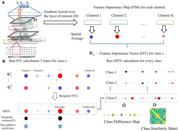
Here we introduce DeepResolve, a gradient ascent based visualization framework for feature map interpretation. DeepResolve computes and visualizes feature impor-tance maps and feature imporimpor-tance vectors which describe the activation patterns of channels at a intermediate layer that maximizes a specific class output. We show that even though gradient ascent methods are less informative when used to gener-ate representations in input space, gradient methods are very useful when conducted in feature map space as a tool to interpret the internal logic of a neural network. By using multiple random initializations and allowing negative values, we explore the feature space efficiently to cover the diverse set of patterns that a model learns about a class. A key insight of DeepResolve is that the visualization of the diverse states of an internal network layer reveals complex feature contribution patterns (e.g. negatively contributing or non-linearly contributing features) and combinatorial fea-ture interactions which can not be easily achieved using other existing visualization tools that operate on input space. The correlation of the positive feature importance vector for distinct classes reveals shared features between classes and can lead to an understanding of shared mechanism. Our automatic pipeline is capable of generating analysis results on feature importance, feature interactions and class similarity, which can be used for biological studies. DeepResolve requires no input dataset or massive post-processing steps and thus is spatially efficient.

2.2

Methods

2.2.1

Visualizing feature importance and combinatorial

in-teractions

Class Specific Feature Importance Map and Feature Importance Vector Unlike methods which use gradient-ascent to generate sequence representations in the input layer[24, 32] , DeepResolve uses gradient-ascent to compute a class-specific optimal feature map Hcin a chosen intermediate layer L. We maximize the objective function:

Hc“ arg max H

ScpHq ´ λ||H||22

Scis the score of class c, which is the c-th output in the last layer before transformation to probability distribution (before sigmoid or soft-max). The class-specific optimal

feature map is Hc P RKˆW for a layer having K feature maps of size W (W is the

width of the feature maps after max-pooling and W “ 1 when global max-pooling is used). K is the number of sets of neurons that share parameters. Each set of neurons that share parameters is called a channel, and each channel captures unique local

features within a receptive field. We name Hc a feature importance map (FIM) for

class c, and each map entry pHk

iqcevaluates the contribution of a neuron from channel k in a specific position i in a layer. When local max-pooling is used, a FIM is capable of capturing the spatial pattern of feature importance within each channel. In typical biological genomic neural networks, spatial specificity is in general low because of the stochasticity in input feature locations. Therefore we compute a feature importance score φk_c for each of the K channels by taking the spatial average of the feature

importance map pHk_q

c of that channel. These scores collectively forms a feature importance vector (FIV) Φc“ ppφ1cq, pφ2cq, ..., pφkcqq:

φk_c “ 1 W W ÿ i“1 pH_ikqc

Note that although the natural domain of feature map is R`

0 if ReLU units are used, we allow FIMs to have negative values during gradient ascent so as to distin-guish channels with negative scores from those with close to zero scores. The feature

importance score for each channel represents its contribution pattern to the output prediction and a channel can contribute positively, negatively or trivially. Positive channels usually associate with features that are ‘favored’ by the class, whereas nega-tive channels represents features that can be used to negate the prediction. We found that negative channels contain rich information about the reasoning of network deci-sions. Negative channels can capture patterns that do not exist in positive samples or non-linearly interacting patterns.

Visualizing complex feature contribution patterns and interactions

Since deep neural networks have the capacity to learn multiple patterns for a single class, the learned function space can be multimodal. Moreover, the channels may contribute differently in different modes and their contributions may condition on the other channels, which indicate complex feature contribution patterns and inter-actions. However an input dependent visualization method usually explores only one of the modes when a specific sample is given. To explore the optimums in the space more efficiently, we repeat gradient ascent multiple times (T times) for each target class c using different random initialization sampled from normal distribution. This generates an ensemble of FIMs tHt

cu and FIVs tΦtcu for each class.

To reduce the effect of bad initializations we weight each gradient ascent result using the output class score. We add an offset to the scores such that all trials have non-negative weights. The ensemble of FIVs exhibits diverse representations of feature space patterns learned by the corresponding class, with some channels having more inconsistent contribution than others. We evaluate the weighted variance of the feature importance score of each channel k in the ensemble, and use it as a metric to evaluate the inconsistency level (IL) of the channel k for target class c:

ILk_c “ Varrpφk_cqts

Channels with a low inconsistency level contribute to the output either positively, negatively, or not at all. We define this type of channel as a additive channel because their contributions can be combined additively (e.g. AND/OR/NOT logic). We define channels with high inconsistency as non-additive channels since their contribution is

Gradient Ascent over the layer of interest (H)

ACCGTTACGGGATCTT

H

…

: Feature Importance Vector (FIV) for class c

…

Feature Importance Map (FIM) for each channel A

… …

Integrate FIVs Run FIV calculation T times for class c

Channel 1 Channel 2

…

Weighted variance(IL)

Favored Unfavored

OFIV

…

Class Similarity Matrix Class Difference Map

Class 1

Class 2

Class C

…

Run OFIV calculation for every class B

Non-additive prediction

Figure 2-1: Illustration of DeepResolve’s working flow.(A) Feature Importance Vectors calculation. After a network is trained and a intermediate layer is selected, DeepResolve first computes the feature importance maps (FIM) of each of the chan-nels using gradient ascent. Then for each channel, the Feature Importance Vector (FIV) score is calculated as the spatial average of its FIM scores. (B) Overall Feature Importance Vector calculation. For each class, DeepResolve repeats the FIV calcu-lation T times with different random initializations. The weighted variance over the T times is then calculated as an indicator of inconsistency level (IL) of each channel. A Gaussian Mixture Model is trained on IL scores to determine the non-additiveness of a channel. For each channel, the T FIVs are combined with the reference to the inconsistency level to generate an Overall Feature Importance Vector (OFIV) which summarizes all ‘favored’ and ‘unfavored’ patterns of a class. Finally, we use the non-negative OFIVs of each class to analyze class similarity and the OFIVs to analyze class differences.

inconsistent and usually conditioned on the other channels (e.g. XOR logic). We visualize the signs and magnitudes of FIV scores of the entire ensemble of FIVs as shown in Figure 2-1 and Figure 2-2. In this way both individual and combinatorial interactions between channels can be easily perceived. In the results section below we show the effectiveness of this visualization using synthesized data in discovering

XOR logic where two channels always have opposite contributions.

Summarizing feature contributions using Overall Feature Importance Vec-tor

We summarize the contribution of a feature using an overall feature importance vector (OFIV) ¯Φcthat takes into account the rich information of the magnitude and direction of the feature contribution embedded in the ensemble of FIVs.

We first calculate the weighted variance of the FIVs for each channel to get the inconsistency level (IL). Three Gaussian mixture models with the number of compo-nents varying from one to three are fitted over the IL scores to account for channels that are additive and non-additive. The final number of mixture components is picked to minimize the Bayesian Information Criterion (BIC).

We next categorize the channels by IL score and the sign of contribution to calcu-late category-specific OFIVs that properly characterizes the feature importance. The channels in the mixture component with the lowest mean are considered as either additive or unimportant. The remaining mixture components (if any) are considered as non-additive channels and can be further categorized by whether the sign of its FIVs in the ensemble is consistent. For channels considered as additive, unimportant, or non-additive with consistent sign, the OFIV is calculated as the weighted average of its scores across all FIVs. For channels considered as non-additive with inconsis-tent sign, the OFIV is calculated as the weighted average of the positive FIVs in the ensemble to reflect the feature contribution in cases where the channel is not used to negate the prediction.

Visualizing OFIVs and IL scores together, we recover both the importance level of different features and the presence of non-additive channels. We automatically produce a list of important features, and a list of non-additive features that are highly likely to involved in complex interactions.

2.2.2

Visualizing feature sharing and class relationship

The weight sharing mechanism of multi-task neural networks allows the reuse of features among classes that share similar patterns. In past studies, the weight matrix

in the last layer has been used to examine class similarity. However, this is potentially problematic because the high-level features in a network’s last layer tend to be class-specific. This method also fails to discover lower level feature sharing between classes that are rarely labeled positive together. Using OFIVs proposed above, we revisit the feature sharing problem to enable the discovery of lower-level feature sharing when the class labels are poorly correlated.

We observe that the network learns to use negative channels to capture class-specific patterns in other classes as a process of elimination to maximize the prediction accuracy. This potentially increases the distance of those classes in hidden space despite the fact that they may share other features. Thus, while neurons with both strong positive and negative OFIV scores are potentially important for making the prediction, only the ones with positive OFIV scores are truly associated with the target class. Inspired by this finding, we introduce a class similarity matrix A by taking pair-wise Pearson correlation of non-negative OFIV of all the classes.

ACiCj “ Covp ¯Φ` ci, ¯Φ ` cjq σ_Φ¯` ciσΦ¯`cj ¯ Φ`

c encodes the composition of all positive contributing features for a given class in intermediate layer. By taking the difference of OFIV of a pair of classes, we can also generate a class difference map.

DCiCj “ ¯Φci´ ¯Φcj

This map highlights features that are favored by one class but not favored by the other. This is especially helpful when studying cell-type specific problems where a key feature deciding differential expression or binding in different cell type might be crucial.

2.2.3

Implementation details

We trained all of our models with Keras version 1.2 and the DeepSEA network is downloaded from the official website. We convert the torch DeepSEA model into Caffe using torch2caffe and the resulting model has same performance as the original

network. We implemented DeepResolve for both Caffe and Keras. As baselines, we implemented saliency map and DeepMotif in Keras, and used DeepLIFT v0.5.1 for generating DeepLIFT scores.

2.3

Results

2.3.1

Synthetic datasets

Recovering important features and combinatorial interactions

We tested if FIVs would highlight important features and identify complex feature interactions in a synthetic data set which contains both additive and non-additive combinatorial logic. Synthetic dataset I contains 100,000 DNA sequences, each con-taining patterns chosen from CGCTTG, CAGGTC and GCTCAT in random positions. We label a sequence 1 only when CAGGTC and one of (GCTCAT,CGCTTG) present, and other-wise 0. This is the combination of AND logic and XOR logic. We also include 20,000 sequences that are totally random and label them as 0. We trained a convolutional neural network with a single convolutional layer with 32 8bp filters and local max-pooling with stride 4, followed by a fully connected layer with 64 hidden units. 20% of the data were held out as a test set and the resulting test AUC was 0.985. We applied DeepResolve on the layer in between convolutional layer and fully connected layer, and each channel correspond to a convolutional filter that can be visualized as Position Weight Matrix after normalization.

As shown in Figure 2-2, when ranked by OFIV, the top filters predicted to be non-additive capture CGCTTG and GCTCAT, the pair of motifs that non-linearly (XOR) interact with each other. The top filters predicted to be additive characterize CAGGTC, the motif that additively (AND) interacts with the other ones. Furthermore, the FIVs correctly unveil the non-additive XOR interaction between GCTCAT and CGCTTG as the corresponding filters tend to have opposite signs all the time. The optimal number of Gaussian mixture components of the IL score is 3 (Figure 2-3), indicating the existence of non-additiveness.

We further compared three types of input-dependent visualizations: DeepLIFT, saliency map, and saliency map multiplied by input. For our comparison we used

Non-additive prediction OFIV —Positive — Negative Run Inde x

Channel Index Feature Importance Vector Run 1-10

Channel a: a b c d e f g Channel b: Channel c: Channel d: Channel e: Channel f: Channel g:

Ground truth logic for the target class: CAGGTC AND (GCTCAT XOR CGCTTG)

Predicted non-additive filters:

Predicted top additive filters:

Variance

Figure 2-2: Illustration of the generation of OFIV from FIVs generated by all 10 runs of gradient ascent in synthetic data set I. Red circles on the X-axis represent positive channels and blue circles represent negative channels. Circle size is proportional to the absolute FIV value. The weighted variance (IL score) of each channel is plotted below the FIVs, where the darkness and circle size is proportional to the variance. The OFIV is visualized below, where the circle size reflect the overall importance score of a channel. The channels that are predicted as non-additive by the Gaussian Mixture Model fitted on the IL scores are labeled by a star. A seqlogo visualization of the filter weight is plotted next to the corresponding channel. Filter {a,f} and {c,d} which capture sequences that involve in XOR logic are correctly predicted as non-additive. Among the remaining filters, the top-OFIV ones {b,c,g} which capture the sequence that involve in AND logic are correctly predicted as additive.

positive and negative examples from synthetic dataset I, where the positive example contains GCTCAT and CAGGTC, and the negative example contains all three patterns. The network prediction on these examples are correct, suggesting that it has learned the XOR logic. Note that the original saliency map takes the absolute value of the gradients which never assign negative scores and thus limits the interpretation of the internal logic of a network. Thus we used the saliency map without taking the absolute value to allow for more complex visualizations. We compute attribution scores for each base pair in the input with regard to the positive class’s softmax logit. As shown in Figure 2-4, the visualization on positive example can be biased by the choice of input since only the 2 patterns that present in the input will be highlighted and the

Figure 2-3: Distribution of optimal number of Gaussian mixture component of variances in each set of experiments. 1 means all the channels are linearly contributing to the class, whereas a value larger than 1 means some of the channels are potentially non-linear. Consistent with the ground truth, for Synthetic I all the classes have both linear and non-linear channels, and for Synthetic II all the classes only have linear channels. For the networks trained on 422 TF binding datasets, 420 only have linear channels. For DeepSEA, 917 out of the 919 classes only have linear channels.

third pattern is always missing. On the other hand, when a negative example is used as input, all three methods assign scores with the same signs to all three patterns, making the XOR logic indistinguishable from AND logic. DeepLIFT assigns positive score to both GCTCAT and CAGGTC even though their co-existence lead to negative

prediction. Moreoever, the saliency methods incorrectly assign negative score to

CAGGTC which is designed to always exists in positive class. This shows that saliency methods can be unstable in attributing positively contributing patterns when complex non-linear logic exists.

Recovering class relationships

We synthesized dataset II to test our ability to discover feature sharing when the labels are poorly correlated. Synthetic dataset II has 4 classes of DNA sequences with one class label assigned to each sequence. Class 1 contains GATA and CAGATG,

Input Sequence

Input-dependentvisualizations only capture 2 ofthe

predefined patterns when only given one positive example. ICGCTTG nput-dependentand GCTCAT visualizatand ions prfoduce ailto iunstllustablrate e vithe sualXOR izatiinton erwiactth ion unfbetixed weensigns. DeepLIFT

Saliency map (withouttaking absolute values)

Saliency x input

Figure 2-4: Input-dependent visualizations produce unstable results on XOR logic and fail to capture the XOR interaction. Three types of input-dependent visualizations on example positive and negative sequence from synthetic data set I. The visualization using positive example (left) only highlight two of the 3 predefined patterns because a positive sample can only contain one of GCT-CAT,CGCTTG, while the third pattern will always be missing. When using negative example which contains all three patterns as the input, all of the methods assign either all positive or all negative scores to the three patterns (right), failing to cap-ture the XOR interaction between GCTCAT and CGCTTG. The saliency methods predict negative score for CAGGTC, a pattern that should always exists in positive examples, suggesting that these methods are not stable enough when dealing with complex logic.

class 2 contains TCAT and CAGATG, Class3 contains GATA and TCAT, while class 4 only contains CGCTTG. The introduced sequence patterns are deliberately selected such that three of the classes share half of their patterns, while class 4 is totally different. These four classes are never labeled as 1 at the same time, thus the labels yield zero information about their structural similarities. We trained a multi-task CNN with a single convolutional layer that has 32 8bp long filters, one fully connected layer with 64 hidden neurons, and a four-neuron output layer with sigmoid activation to predict the class probability distribution. The test AUC is 0.968, 0.967, 0.979, 0.994 for class 1 to 4.

Figure 2-5(A) shows the OFIV for each of the classes, and the optimal number of Gaussian mixture components of the IL score for all of the classes is one (Fig-ure 2-3), correctly indicating that only additive channels exist in these classes. We observe that the channels with the top OFIV (red) correctly capture the sequence

Overall Feature Importance Vector for each class Class 1: GATA + CAGATG Class 2: CAGATG + TCAT Class 3: GATA + TCAT Class 4: CGCTTG Channel Index

A B Positive OFIV correlation Class label correlation

Last layer weight dot product OFIV correlation

Figure 2-5: Visualization of DeepResolve in multi-task networks. (A)Overall Feature Importance Vector for Synthetic dataset II class 1 - 4. Each circle on the X-axis represents a channel, with red representing positive OFIV score and blue repre-senting negative OFIV score. Each column corresponds to one of the 32 channels that is shared among all four classes. OFIV successfully ranks predefined sequence fea-tures as the most important feafea-tures for each of the classes, while reveals ‘unfavored’ features that are used to separate a class from its competing classes.(B)Correlation matrix of class based features shows the benefit of non-negative OFIV scores. The predefined sequence pattern for each class is shown (A). Our proposed Class Similar-ity Matrix (top-left) successfully assigns high correlation to (Class1, Class2), (Class2, Class3) and (Class1, Class3) and low correlation to all pairs with Class 4. The ma-trix in top right corner suggest low correlation between the labels of each class. The matrix on the bottom left is the Pearson correlation of ONIV score without removing the negative terms, and the bottom right matrix is calculated by taking the cosine of the corresponding rows in last layer weight matrix. The bottom two both fail to assign higher similarity score to combinations of classes that share sequence features.

determinants of the corresponding class. We observe strong negative terms (blue) in OFIVs for all classes, representing sequence patterns ‘favored’ by other alternative classes, which validates our hypothesis that the ’process of elimination’ truly exists. Figure 2-5(B) compares class similarity matrices generated by our method and using the last layer weight matrix. The non-negative OFIV correlation matrix successfully assigned higher similarity score to class 1+2, class 1+3 and class 2+3, while the other methods failed to do so. Note that for class 1+3 and class 2+3, the similarity scores estimated by the last layer weight dot product are strongly negative, suggesting that the same features will lead to the opposite predictions between these pairs of classes. While consistent with label correlation , this interpretation is contradictory to the

fact that those classes are actually similar in feature composition, showing limitations of conventional methods that are based on the last layer weight. The correlation when using both positive and negative ONIV scores suggest similar pattern as the last layer weight, showing that the negative terms confounds the similarity analysis.

2.3.2

Experimental datasets

We analyzed two experimental datasets to examine DeepResolve’s ability to recover biologically important features, and to discover correlation in features that might relate to mechanism.

Identifying key motifs in models of TF binding

We applied DeepResolve to convolutional neural networks trained on 422 Transcrip-tion Factor ChIP-Seq experiments for which the TF motifs are available in the non-redundant CORE motifs for vertebrates in JASPAR 2015 ([9, 8]) and only one motif exists for each TF. The positive set contains 101-bp sequences centered at motif in-stances that overlap with the ChIP-seq peaks. For each TF, the JASPAR motif for the corresponding factor (Supplementary Table 1) is used to identify motif instances using FIMO. The negative set are shuffled positive sequences with matching dinu-cleotide composition. Each sequence is embedded into 2-D matrices using one-hot encoding. We train a single-class CNN for each experiment using one convolutional layer with 16 filters of size 25 with global max-pooling, and 1 fully connected layer with 32 hidden units. The mean of the AUC for these 422 experiments is 0.937 and the standard deviation is 0.035. We then generate FIMs and OFIVs for each experiment on the last convolutional layer, and rank the filters using OFIV scores. 420 of the 422 experiments contain only additively contributing features (Figure 2-3).We convert the top filters into position weight matrices (PWMs) and match them with known motif for the target TF using TOMTOM [34], and count how many times we hit the known motif in top 1, top 3 and top 5 filters with matching score p-value less than 0.5 and 0.05. We compare our method to DeepMotif ([32]), a visualization tool that generates important sequence features by conducting gradient ascent directly on the input layer. We improved DeepMotif’s initialization strategy to allow multiple random

initializa-tions instead of using an all 0.25 matrix (naming it enhanced-DeepMotif), and take the most informative 25bp fragment of generated sequences with top 5 class score. We also compared with three gradient-based methods, deepLIFT,saliency map, and its variation where the gradients are multiplied by the inputs to the neurons. However we conducted them on an intermediate layer instead of on input layer. We used all sequences from the positive training set, and took the average of scores assigned to a channel as an indication of the importance of a channel.

Top 1 Top 3 Top 5 Ranksum Wilcoxon

TOMTOM P-value 0.5 0.05 0.5 0.05 0.5 0.05 p-values p-values

DeepResolve (ours) 412 407 421 418 422 421 N/A N/A

DeepLIFT 418 418 420 420 421 421 0.784 0.412

Saliency*activation 404 393 419 419 420 420 7.478 ˆ 10´7 _{1.049 ˆ 10}´9

Saliency 388 377 417 416 420 420 4.63 ˆ 10´7 _{4.63 ˆ 10}´15

enhanced DeepMotif 217 89 310 123 343 147 N/A N/A

Table 2.1: Top-1, top-3, top-5 accuracy in identifying matching motif for TF binding (out of 422 experiments) with similarity score (p-value) smaller than 0.5 and 0.05, and the paired/unpaired rank tests of the proposed ranks of best matching filters between our method and the input-dependent methods.

Shown in Table 2.1, our method successfully proposes known matching motifs as top 5 features in all of the 422 experiments with TOMTOM p-value less than 0.5, and in 421 out of 422 experiments with p-value less than 0.05, which outperforms enhanced DeepMotif by „3-fold. Our method also outperforms saliency map and its variation in top-1, top-3, top-5 accuracy, and outperforms deepLIFT in top-3, top-5 accuracy with TOMTOM p-value less than 0.5. We selected the top filter that matched a known canonical motif with lowest TOMTOM p-value from each exper-iment, and conducted Mann-Whitney Ranksum (unpaired) and Wilcoxon (paired) rank test between the ranks that DeepResolve and input-dependent methods assign to these filters. Our method is significantly better (p ă 0.000001) then the saliency map method and its variation on both tests and is comparable to DeepLIFT even though we did not refer to any input dataset when calculating our OFIVs. The distri-bution of optimal numbers of Gaussian mixture components for all the experiments is plotted in Figure 2-3, where only 2 of the experiments have potentially non-additive channels. This result demonstrates that the logic for single TF binding is mostly additive and complex feature interactions such as XOR logic are unlikely. It also

shows that the convolutional filters in genomic studies can capture motifs accurately by themselves, which lays a good foundation for hierarchical feature extraction and interpretation tools like DeepResolve.

Figure 2-6: Distribution of positive sample activation level, negative sample activation level and motif matching p-values of filters grouped by their ONIV score ranking. We collected convolutional filters from all 422 TF binding models and group them into four groups by the ranks of ONIV score, each containing 1688 filters. Each panel represents one of the groups and the ONIV ranks increase from left to the right. The averaged activation scores across all negative and positive examples are calculated for each filter, and is normalized to [0,1] within each network. The top ranking group (right most) has high activation in positive examples while low activation in negative examples, and has the most significant motif matching pvals. This is suggesting that DeepResolve ranks highly relevant and informative filters that can separate positive and negative set well.

We further analyzed the learned convolutional filters from all 422 TF binding models by visualizing their activation patterns and relevance to known motifs. We grouped them into four groups by the ranks of ONIV score and plotted the distribution of the averaged activation scores across all negative and positive examples. We also plotted the distribution of TOMTOM p-values of the corresponding motif for each

group. As shown in Figure 2-6, the top ranking group (right most) has highest

activation in positive examples and lowest activation in negative examples, and has the most significant motif matching p-values. This suggest that ONIV successfully selected highly relevant and informative filters that can separate the positive and negative sets.

Identifying sequence feature sharing and class correlations in DeepSEA We evaluated DeepResolve’s ability to discover important features and identify shared features and class similarities across distinct classes in the DeepSEA network[10], a classic multi-task convolutional network trained on whole genome data to predict 919

different features including chromatin accessibility, TF binding and histone marks across a variety of cell types. DeepSEA compresses a large training set into its pa-rameters and thus we sought to interpret DeepSEA’s papa-rameters to uncover biological mechanism. To p m at ch in g JA SP A R m ot if s

480 Channel in 2nd convolutional layer

Channel Feature Visualization Top matching motif

Channel #116 _Alx4

Channel #280 Myod1 GATA2

Channel #77 NFYB/YA Reverse comp. MafG Channel #451 Channel #179_1 Channel #179_2 REST REST reverse comp.

GATA1:: TAL1 NFYB/YA

Figure 2-7: Visualization of sequence features captured by the 480 channels in 2nd convolutional layer of DeepSEA. The sequences are generated using gra-dient ascent (see section 2.3.2). The matrix represents -log10 of TOMTOM Q-values for each pair of channel and its top matching motifs. Each row represents a known JASPAR motif which has been ranked as top 1 matching motif for at least one of the channels. Only pairs that achieve less than 0.005 Q-value are represented with actual Q-value, and the dark blue region represents default value for low Q-values. In the right panel, the left column shows the SeqLogo visualizations of representative gradient ascent outputs of 5 of the channels, and the top matching motifs are shown in the right column. Channel 116 and 451 captures single motif of Alx4 and MafG. Channel 280 captures 3 consecutive motifs (GATA1,Myod1 and GATA2), while chan-nel 77 captures consecutive NFYB/YA motif and its reverse compliment. Chanchan-nel 179 captures either REST or its reverse compliment depending on the input sequences used for initialization.

In DeepSEA, input sequences are 1000bp long, and the labels are 919 long binary vectors. The network has 3 convolutional layers with 320, 480, 960 filters, and 1 fully connected layer. We chose the input to the 3rd convolutional layer as H to generate feature importance maps, where the activation of a channel is determined by a 51bp sequence segment in the input (receptive field). We visualized the sequence features of a channel by l2-regularized gradient ascent over its receptive field to maximize the channel activation. We initialized the input with the top ten 51bp fragment from the training sequences that maximize the channel activation. We applied a heuristic thresholding to the optimized input segments and normalized them to sum up to one

in each column, and used TOMTOM to compare the resulting position weight matrix with known JASPAR motifs. Figure 2-7 left panel shows the -log10 of the TOMTOM Q-values for each pair of channel and its top matching motifs. We discovered 218 channels that capture sequence features that match with 200 known JASPAR motifs with Q-value smaller than 0.005, and we observed channels that capture single motif, multiple motifs, consecutive motif with its reverse compliment (Figure 2-7). We show that a single channel can capture both a motif and its reverse compliment depending on the input sequences, and we captures this dynamic by using multiple initializations for the gradient ascent.

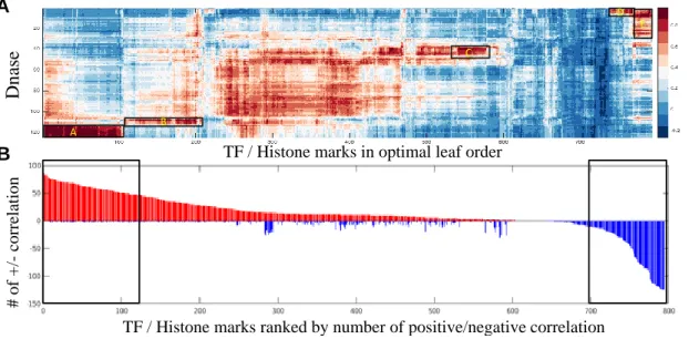
We next computed a class similarity matrix based upon OFIVs and found that the resulting matrix revealed similarities between the decision functions that underlie distinct classes, even when the classes themselves were not strongly correlated. We first calculated FIVs and their weighted variances for each class. The distribution of optimal numbers of Gaussian mixture components for all the experiments is plotted in Figure 2-3, where only 2 of the experiments have potentially non-additive channels. This indicates that the majority of the classes in DeepSEA employ additive logic where binding can be determined by the additive contribution of several motifs. We then generated a class similarity matrix as described in Section 2.2.2. Given that DeepSEA takes in 1000bp long sequences around the biological event, it captures upstream and downstream sequence context. Therefore our proposed metric measures similarities between the contextual structures of a pair of regulators, which could imply interesting correlations in functionality and mechanism. Figure 2-8 compares DeepResolve’s class similarity matrix with the label correlation matrix and the dot product matrix of last layer weights for all classes. DeepResolve’s class similarity matrix revealed strong correlation between pairs of TFs/histone marks/DNase hypersensitivity that do not necessarily co-appear within 200 bp or having strong last layer weight correlation, but are functionally relevant.

We then examined the correlation pattern between selected TF/histone marks and DNase I hypersensitivity across different cell types to explore the shared com-ponents of their decision functions. Figure 2-9(A) shows the bi-clustering result on the TF-histone mark/DNase similarity matrix. We observed clusters of TFs and histone marks sharing similar patterns, and some of them exhibit cell-type specific