The Cryosphere, 7, 1227–1245, 2013 www.the-cryosphere.net/7/1227/2013/
doi:10.5194/tc-7-1227-2013
© Author(s) 2013. CC Attribution 3.0 License.
EGU Journal Logos (RGB) Advances in
Geosciences
Open Access
Natural Hazards and Earth System Sciences
Open Access
Annales Geophysicae
Open Access
Nonlinear Processes in Geophysics
Open Access
Atmospheric Chemistry and Physics
Open Access
Atmospheric Chemistry and Physics
Open Access
Discussions
Atmospheric Measurement
Techniques
Open Access
Atmospheric Measurement
Techniques
Open Access
Discussions
Biogeosciences
Open Access Open Access
Biogeosciences
Discussions
Climate of the Past
Open Access Open Access
Climate of the Past
Discussions
Earth System Dynamics
Open Access Open Access
Earth System Dynamics
Discussions
Geoscientific Instrumentation
Methods and Data Systems
Open Access Geoscientific
Instrumentation Methods and Data Systems
Open Access
Discussions
Geoscientific Model Development
Open Access Open Access
Geoscientific Model Development
Discussions
Hydrology and Earth System
Sciences
Open Access
Hydrology and Earth System
Sciences
Open Access
Discussions
Ocean Science
Open Access Open Access
Ocean Science
Discussions
Solid Earth
Open Access Open Access
Solid Earth
Discussions
The Cryosphere
Open Access Open Access
The Cryosphere
Discussions
Natural Hazards and Earth System Sciences
Open Access
Discussions
Reanalysing glacier mass balance measurement series
M. Zemp 1 , E. Thibert 2 , M. Huss 3 , D. Stumm 4 , C. Rolstad Denby 5 , C. Nuth 6 , S. U. Nussbaumer 1 , G. Moholdt 7 , A. Mercer 8 , C. Mayer 9 , P. C. Joerg 1 , P. Jansson 8 , B. Hynek 10 , A. Fischer 11 , H. Escher-Vetter 9 , H. Elvehøy 12 , and L. M. Andreassen 12
1 Department of Geography, University of Zurich (UZH), Zurich, Switzerland
2 IRSTEA, UR ETGR Erosion Torrentielle, Neige et Avalanches, Saint-Martin-d’H`eres, France
3 Department of Geosciences, University of Fribourg (UFR), Fribourg, Switzerland
4 International Centre for Integrated Mountain Development (ICIMOD), Kathmandu, Nepal
5 Department of Mathematical Sciences and Technology, The Norwegian University of Life Sciences (UMB), ˚ As, Norway
6 Department of Geosciences, University of Oslo (UiO), Oslo, Norway
7 Scripps Institution of Oceanography, University of California, San Diego, USA
8 Department of Physical Geography and Quaternary Geology, Stockholm University, Stockholm, Sweden
9 Commission for Geodesy and Glaciology, Bavarian Academy of Sciences and Humanities, Munich, Germany
10 Zentralanstalt f¨ur Meteorologie und Geodynamik (ZAMG), Vienna, Austria
11 Institute for Interdisciplinary Mountain Research, Austrian Academy of Sciences, Innsbruck, Austria
12 Norwegian Water Resources and Energy Directorate (NVE), Oslo, Norway Correspondence to: M. Zemp ([email protected])
Received: 1 February 2013 – Published in The Cryosphere Discuss.: 4 March 2013 Revised: 10 June 2013 – Accepted: 21 June 2013 – Published: 6 August 2013
Abstract. Glacier-wide mass balance has been measured for more than sixty years and is widely used as an indicator of climate change and to assess the glacier contribution to runoff and sea level rise. Until recently, comprehensive un- certainty assessments have rarely been carried out and mass balance data have often been applied using rough error esti- mation or without consideration of errors. In this study, we propose a framework for reanalysing glacier mass balance series that includes conceptual and statistical toolsets for as- sessment of random and systematic errors, as well as for vali- dation and calibration (if necessary) of the glaciological with the geodetic balance results. We demonstrate the usefulness and limitations of the proposed scheme, drawing on an anal- ysis that comprises over 50 recording periods for a dozen glaciers, and we make recommendations to investigators and users of glacier mass balance data. Reanalysing glacier mass balance series needs to become a standard procedure for ev- ery monitoring programme to improve data quality, including reliable uncertainty estimates.
1 Introduction
Changes in glacier mass are a key subject of glacier mon- itoring, providing important information for assessing cli- matic changes, water resources, and sea level rise. The most extensive dataset of glacier-wide in situ mass balance mea- surements covers the past six decades (WGMS, 2012; and earlier volumes) and is widely used to assess global glacier changes (e.g. Cogley, 2009) and related consequences of re- gional runoff (e.g. Weber et al., 2010) and global sea level rise (e.g. Kaser et al., 2006). However, most of these data se- ries consist of just a few observation years, and most results are reported without uncertainties (Zemp et al., 2009).
There are a dozen mass balance programmes with contin- uous time series dating back to 1960 or earlier on relatively small mountain and valley glaciers (Zemp et al., 2009). Com- bined with multi-annual geodetic surveys, these long-term glaciological mass balance series provide a unique opportu- nity for quantitative assessment of the related uncertainties.
Earlier works found both agreement (e.g. Funk et al., 1997)
and disagreement (e.g. Østrem and Haakensen, 1999) be-
tween the mass balance results from the two methods. Recent
studies have carried out extensive homogenization and un- certainty assessments for reanalysing mass balance series (e.g. Thibert et al., 2008; Rolstad et al., 2009; Huss et al., 2009; Koblet et al., 2010; Fischer, 2010, 2011; Zemp et al., 2010; Nuth and K¨a¨ab, 2011; Andreassen et al., 2012). How- ever, there are no guidelines available yet for standardization of the process, and a direct comparison of the findings from the above studies is challenging.
In the summer of 2012, a workshop organized by the World Glacier Monitoring Service (http://www.wgms.ch) in collaboration with Stockholm University was held on “Mea- surement and Uncertainty Assessment of Glacier Mass Bal- ance” at the Tarfala Research Station in northern Sweden (Nussbaumer et al., 2012). The workshop built upon results and experience of earlier workshops at Tarfala in Sweden (GAA, 1999) and Skeikampen in Norway (IGS, 2009) and brought together a group of experts currently working on these issues. Its major goals were to discuss methods and re- lated uncertainties of glaciological and geodetic mass bal- ance measurements and to find a consensus on best prac- tices, mainly for homogenization, validation, and calibration of (long-term) observation series.
The present paper is a joint outcome of that workshop and aims at proposing best practices for reanalysing mass balance series. First, we provide a brief review of obser- vation methods, related uncertainties, and reanalysing pro- cedures for observation series. Second, we present results from a select number of glaciers with long-term mass bal- ance programmes and discuss these in light of the proposed reanalysing scheme. Finally, we conclude with recommenda- tions for data producers and summarize implications for data users.
2 Theoretical background
2.1 Terminology and components of glacier mass balance
A common language and terminology is a basic requirement for developing any best practice. In this work, the terminol- ogy (in English), formulations, and units of measurement follow the “Glossary of Glacier Mass Balance and Related Terms” of Cogley et al. (2011). “Homogenization” and “re- analysis” of observational data series are well established in climatology (cf. Kalnay et al., 1996; Aguilar et al., 2003;
Begert et al., 2005). However, the corresponding methods, developed for treating an atmospheric continuum, cannot be directly applied to discrete glaciers. We, hence, use these terms in their general climatological meaning but specify the methodological implementation for glacier mass balance se- ries in Sect. 3. In the same chapter, general definitions and glacier-specific explanations are given for “validation” and
“calibration”, which are used differently among communi- ties. In terms of the uncertainty assessment, we differentiate
between random (i.e. noise) and systematic (i.e. bias) errors (i.e. disagreements between measured and true values).
The mass balance of a glacier is defined as the sum of all components of accumulation (acc) and ablation (abl), and a distinction can be made between surface (sfc), internal (int), and basal (bas) balances (see Table 1 and Fig. 2 in Cogley et al., 2011). Based on the conservation of mass within a col- umn of square cross section extending in the vertical direc- tion through the glacier, the mass-balance rate of the column is
m ˙ = ˙ acc
sfc+ ˙ abl
sfc+ ˙ acc
int+ ˙ abl
int+ ˙ acc
bas+ ˙ abl
bas+ q
in+ q
outds , (1) with q referring to the flow of ice into or out of the column with fixed horizontal dimension, ds = dx dy.
The point mass balance cumulated over one year b a (or more generally over the span of time from t 0 to t 1 ) is linked to the mass balance rate by
b a = m (t a ) − m (t 0 ) =
t
aZ
t
0m (t ) ˙ dt . (2)
To obtain the glacier-wide mass balance, the point balances are integrated over the glacier mean area S over the same time span:
B a = 1 S ·
Z
S
b a ds. (3)
Note that this study focuses on land-terminating glaciers;
the balance components of lake and marine floating glacier tongues and ice shelves are not considered here because their mass balance is often dominated by frontal and basal terms not addressed by the glaciological method (cf. Kaser et al., 2003).
2.2 Glaciological observation method
The principal steps of the glaciological observation method
are the measurement of ablation and/or accumulation at in-
dividual points as well as the interpolation between the mea-
surement points and extrapolation to unmeasured regions of
the glacier. Often, the interpolation and extrapolation pro-
cess incorporates mass balance indicators, such as snowline
observations and related expert knowledge. The glaciologi-
cal method was described in detail by Østrem and Brugman
(1991) as well as summarized by Kaser et al. (2003) with par-
ticular attention to low latitude glaciers. The basic principles
of the glaciological method are widely accepted and have
not changed much since the earliest measurements. How-
ever, the detailed implementation does vary between differ-
ent glaciers and observers. The number and density of stake
and snow pit observations varies from glacier to glacier and
through time (e.g. Fountain and Vecchia, 1999; Miller and
Pelto, 1999; Van Beusekom et al., 2010). Another typical
variation is the deviation from the traditional contour line method, as proposed by Østrem and Brugman (1991), for the spatial integration of point observations. Often, statistical analysis or interpolation schemes are used instead (e.g. Lli- boutry, 1974; Jansson, 1999) or observed mass balance gra- dients are applied to the glacier hypsometry (e.g. Funk et al., 1997). The direct measurements are typically carried out sea- sonally or annually and cover the components of the surface mass balance. On some glaciers the measurements are per- formed at monthly (on some inner-tropical glaciers) or even at daily resolution (at a few points during summer seasons).
Observers at some cold or polythermal glaciers account for internal accumulation too (e.g. Josberg et al., 2007). The re- sults are usually reported for the mass balance year, refer- ring to the floating-date, the fixed-date, or the stratigraphic time system, and as specific mass balance in the unit metre water equivalent per year (m w.e. a −1 ). Equilibrium line al- titude (ELA), accumulation area ratio (AAR), and mass bal- ance gradients are usually calculated from mass balance dis- tribution with elevation (ranges).
There are three main sources of random and systematic er- rors in the glaciological method: the field measurements at point locations, the spatial averaging of these results over the entire glacier, and the changes of glacier in area and eleva- tion. The field measurements are subject to errors in (i) height determination (e.g. due to measurement precision; tilt, sink- ing and floating of ablation stakes; tilt of snow probings and difficulties in identifying last year’s surface in the snow pack, e.g. due to ice lenses); (ii) density measurement errors and associated assumptions (with errors expected to be larger for snow and firn than for ice); (iii) superimposed ice, which is difficult to measure and of which the spatial variability is often not well captured by the stake network (e.g. Schytt, 1949; Wright et al., 2007); and (iv) flux divergence which is irrelevant to the glacier-wide balance (cf. Cuffey and Pater- son, 2010) unless the sampling between divergence and con- vergence zones is unbalanced (Vallon, 1968). Error sources related to the spatial averaging of the point measurements are (v) the local representativeness of the point measure- ments (i.e. the ability of the observational network to capture the spatial variability of the surface balance; e.g. Fountain and Vecchia, 1999; Pelto, 2000), (vi) the method (e.g. con- tour, profile, kriging) used for interpolation between the point observations and for extrapolation to unmeasured regions (e.g. Hock and Jensen, 1999; Escher-Vetter et al., 2009), and (vii) the under-sampling of inaccessible or difficult glacier ar- eas with potentially different surface balances such as those due to crevasses, debris covers, steep slopes, avalanche zones (e.g. Østrem and Haakensen, 1999). Common to all mass bal- ance series is (viii) The issue of the glacier elevation and area changing over time: the (changing) coordinates and eleva- tion of observation points can directly be measured whereas the glacier area of the most recent geodetic survey is typ- ically used as a constant for the calculation of the specific glaciological balances for the years up until the next geode-
tic survey. Especially for large relative changes, this requires a recalculation of these annual “reference-surface” balances with updated glacier areas (and elevation bands) for every year in order to provide “conventional” balances (cf. Elsberg et al., 2001; Huss et al., 2012). A simple analytical solu- tion to this type of inhomogeneity is given in Sect. 3.2. The few studies which have attempted to quantify all these er- rors include Thibert et al. (2008), Huss et al. (2009), Fischer (2010), Zemp et al. (2010), Hynek et al. (2012), and refer- ences therein.
Observation principles were mainly developed on and for land-terminating, mid-latitude glaciers in the Northern Hemisphere, which mainly change by winter accumulation and summer ablation. In practice, these principles and the relative importance of the error sources listed above might be of limited applicability to the seasonal analysis of glaciers in other regions. However, cumulative annual balances elim- inate these seasonal complexities which, hence, might not be relevant to the following comparison with multi-annual geodetic balances.
2.3 Geodetic observation method
The geodetic observation method determines volume change by repeated mapping and differencing of glacier surface ele- vations. Common methods are ground surveys using theodo- lites (e.g. Lang and Patzelt, 1971) or global navigation satel- lite systems (e.g. Hagen et al., 2005), airborne or space- borne surveys with photogrammetry (e.g. Finsterwalder and Rentsch, 1981; Berthier et al., 2007), and SAR interferome- try (e.g. Magnusson et al., 2005; Berthier et al., 2007) or var- ious forms of laser-altimetry (e.g. Sapiano et al., 1998; Geist et al., 2005; Moholdt et al., 2010). For large ice fields and ice caps, accurate elevation data are often limited to a selection of survey profiles along glacier centre lines or a systematic pattern of ground-tracks from satellite altimetry. A compar- ison with the glaciological balance can be done along com- mon centre lines or after extrapolation to the entire glacier.
The uncertainty and potential bias related to this extrapola- tion (e.g. Arendt et al., 2002; Berthier et al., 2010) need to be accounted for in a similar manner as for the glaciological method. The methodological description below focuses on DEM (digital elevation model) differencing over the entire glacier surface and does not consider extrapolation errors. It also assumes that all elevation data are referenced to the same datum and projection.
Volume changes derived by differencing DEMs can be ex- pressed by the following equation:
1V = r 2 X K
k=1 1h k , (4)
where K is the number of pixels covering the glacier at the
maximum extent, 1h k is the elevation difference of the two
grids at pixel k, and r is the pixel size. Geodetic surveys
are ideally carried out at the end of the ablation season, si-
multaneously with the glaciological survey, and preferably
repeated about every decade. A time separation of about one decade accentuates the detection of a climatic signal and re- duces the impact of short-term elevation fluctuations due to seasonal and interannual meteorological processes. The re- sults of the geodetic method thus refer to the time span be- tween two surveys and are reported as volume change in the unit cubic metre (Eq. 4). Commonly, the geodetic balance is obtained by making an assumption about the density of the volume gained or lost (see Eq. 5 in Sect. 2.4). If it is true that the change of bed elevation is negligible, the geodetic mass balance covers all components of the surface, internal, and basal balances.
Sources of potential errors in elevation data can be catego- rized into sighting and plotting processes. Sighting includes errors that are related to the measurement process and origi- nate from the platform, the sensor and the interference of the atmosphere. Plotting errors relate to the analogue (e.g. map) or digital (e.g. DEM) representation of the sighting results including geo-referencing, projection, co-registration, and sampling density. Additional systematic errors in geodetic volume changes can originate from changing reference areas (e.g. due to frontal fluctuations or ice divide migrations) and from glacier regions not covered by the geodetic survey(s). It is therefore important to keep the glacier masks (and areas) consistent both within and between glaciological and geode- tic analyses. Physical modelling of above errors is only pos- sible with full information on sighting and plotting processes (e.g. Thibert et al., 2008; Joerg et al., 2012), which is often not available.
Alternatively, statistical approaches can be used to assess combined DEM errors by using the population of DEM dif- ferences over non-glacier terrain (assuming it is stable). In contrast to the physical error modelling, this approach in- corporates all known and unknown error sources except er- rors that are spatially consistent in both DEMs. A principal bias in elevation differences is included from misalignment of the DEMs that are differenced. This misalignment trans- lates into a bias in the derived elevation changes and is di- rectly related to the combined slope and aspect distribution of a glacier. Therefore, we recommend performing 3-D co- registration of the DEMs. An analytical relationship and sim- ple solution for DEM misalignment is presented in Nuth and K¨a¨ab (2011), and the procedure is explained briefly in Sup- plement A, Eqs. (A1)–(A4).
In addition to the errors related to the DEM co-registration, an uncertainty exists mainly related to the combined preci- sion of the geodetic acquisition systems. For our statistical approach, the standard deviation of the elevation differences on stable terrain indicates the uncertainty of the DEM dif- ferences for individual pixels. The standard error, defined as the standard deviation divided by the square root of the number of independent items of information in the sample, indicates an uncertainty when spatially averaging the data such as for estimating glacier-wide changes. However, for the calculation of the standard error the number of independent
items cannot be assumed to be equal to the number of items in the sample (i.e. pixels) because spatial auto-correlation is commonly present in elevation data (e.g. Schiefer et al., 2007) and must be accounted for (Etzelm¨uller, 2000). A method to determine the uncertainty related to the spatial auto-correlation based on semi-variogram analysis (σ S in Eqs. B2 and B3) is described in Rolstad et al. (2009), and is summarized briefly in Supplement B.
A final consideration for statistical uncertainty analysis is whether the bedrock terrain surrounding the glacier is repre- sentative of the glacier surface. This depends upon the ele- vation acquisition technique (for example, in photogramme- try, glacier surfaces with low visible contrast may have larger random errors than high-contrast bedrock surfaces), the slope distribution of the surrounding topography versus glacier to- pography (K¨a¨ab et al., 2012), and/or whether the differenced elevation data are of varying resolutions (Paul, 2008).
2.4 Generic differences between glaciological and geodetic mass balance
A direct comparison of glaciological and geodetic balances requires accounting for survey differences (i.e. in time sys- tem and reference areas) and for generic differences between the glaciological and the geodetic balances (i.e. internal and basal balances). The corrections related to the survey differ- ences need to account for ablation and accumulation between the glaciological and the geodetic surveys. Also, both meth- ods must use common reference areas (with regard to ice di- vides and glacier boundary definitions) in order to ensure that results of the same glacier system are being compared. Ac- counting for the generic differences basically means to quan- tify (if possible) the following mass balance components and related uncertainties: internal ablation (including heat con- version from changes in gravitational potential energy), in- ternal accumulation, basal ablation (including ice motion, geothermal heat, and basal melt due to basal water flow), and basal accumulation.
For a comparison with the glaciological balance, the geodetic volume change must be converted into a specific mass balance over a period of record (PoR) in the unit metre water equivalent (m w.e.):
B geod.PoR = 1V S
· ρ
ρ water , (5)
where ρ is the average density of 1V , assuming no change in bulk glacier density over the balance period, and S is the average glacier area of the two surveys at time t0 and t1 as- suming a linear change through time as
S = S t0 + S t1
2 . (6)
Glacier elevation changes are a combined result of changes
in surface, internal, and basal balance, and the flux diver-
gence at a point (Cuffey and Paterson, 2010). Below the
ELA, changes are either ice ablation or emergence, so that the appropriate density is that of ice. In cases with known (observable) firn line changes, the density conversion over the area of firn coverage change can be approximated by an average density of firn and ice over those pixels (Sapiano et al., 1998). In areas with permanent firn cover, the appropri- ate density depends on the relative contributions of surface and dynamical components to the elevation change and is commonly between 500 and 900 kg m −3 . Special cases oc- cur when a change in elevation results solely from firn com- paction or expansion leading to volume changes with no as- sociated mass change or in cases of increasing/decreasing el- evations and firn compaction/expansion with depth, respec- tively, when the mass conversion can be larger than the den- sity of ice. Unless firn pack changes are carefully investigated and/or known, a first approximation is to use a glacier-wide average density together with a plausible uncertainty range, such as ρ = 850 ± 60 kg m −3 (cf. Sapiano et al., 1998; Huss, 2013). If biases are suspected, then sensitivity tests can help to determine the potential magnitude of bias in these density assumptions (e.g. Moholdt et al., 2010; K¨a¨ab et al., 2012;
Nuth et al., 2012; Huss, 2013).
3 Conceptual framework for reanalysing glaciological and geodetic mass balance series
Reanalysis is defined by Cogley et al. (2011) as the re- examination and possible modification of a series of mea- surements in the light of methods or data not available when the measurements were made. In order to avoid confusion with the climatological “reanalysis” product (cf. Kalnay et al., 1996), we use the terms “reanalyse” or “reanalysing” in this paper.
The glaciological method is able to capture the spatial and temporal variability of the glacier mass balance even with only a small sample of observation points (e.g. Lliboutry, 1974; Fountain and Vecchia, 1999) but is sensitive to sys- tematic errors which accumulate linearly with the number of seasonal or annual measurements (Cox and March, 2004;
Thibert et al., 2008). The geodetic balance is able to cover the entire glacier but requires a density conversion and is car- ried out at multi-annual intervals. Hence, the ideal way to re- analyse a mass balance series is to combine the glaciological method with multi-annual geodetic surveys (Hoinkes, 1970;
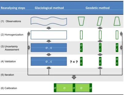
Haeberli, 1998). In the following, we present a compre- hensive scheme for the entire reanalysing process including six principal steps (Fig. 1). The observation step (Sect. 3.1) includes measurements and documentation of glacier mass balance which are subject to methodological and observer- related inhomogeneities. The aim of the homogenization (Sect. 3.2) is to reduce these inhomogeneities whereas the uncertainty assessment (Sect. 3.3) is concerned with the esti- mation of remaining systematic (ε) and random (σ ) errors.
Validation (Sect. 3.4) compares the glaciological with the
geodetic balance. In the event of significant differences, the iteration step (Sect. 3.5) is designed to identify and quantify the corresponding error sources. Should a large difference of an unknown origin be revealed, the glaciological balance is calibrated to the geodetic balance (Sect. 3.6).
3.1 Observations
Observations are generally defined as the recording of measurements and related meta-data. For the glaciological method, observations at stakes and pits are carried out in sea- sonal or annual field surveys and later inter- and extrapolated to derive glacier-wide mass balance. Over the years, the ob- servational set up is subject to various changes, such as in the stake and pit network, in the observers, in inter- and extrapo- lation methods, and in glacier extent. Similar inconsistencies are often present in geodetic data series. Due to the typically decadal intervals the individual surveys are usually carried out with different sensors and platforms, by different opera- tors and analysts, and using different software packages and interpretation approaches. For later reanalysing the observa- tion series, it is important that the related meta-data are stored and made available with the observational results.
3.2 Homogenization
Homogenization is defined as the procedure to correct mea- surement time series for artefacts and biases that are not nat- ural variations of the signal itself but originate from changes in observational or analytical practice (Cogley et al., 2011).
The aim of this step is to use available data and meta-data to detect and reduce inhomogeneities so that the observation se- ries are internally consistent. Both the glaciological and the geodetic data series need to be homogenized independently.
Typical issues for the glaciological method are the change in inter- and extrapolation approaches (e.g. from contour line to altitude profile method), the use of different glacier catch- ments, or the annual (non-)adjustment of changing glacier extents. The latter issue of changing glacier area (and eleva- tion) over time is an inhomogeneity common to all mass bal- ance series. The following approach provides conventional balances by adjusting the surface area and recalculating the specific balance for each elevation band of the glacier.
Assuming a linear area change over a period of record cov- ering N years, the area S of an elevation band e is calculated for each year t as
S e.t = S e.0 + t
N · (S e.N − S e.0 ), (7) with elevation bin areas S e.0 and S e.N from the first and the second geodetic survey, respectively. The time t is zero in the year of the first survey.
The conventional balance for the entire glacier is now
regularly computed as the area-weighted sum of all (E)
Reanalysing steps Glaciological method Geodetic method
(1) Observations ( )
(2) Homogenization (2) Homogenization
(3) Uncertainty σ ε σ σ σ
( ) y
Assessment σ , ε
σ σ σ
ε ε ε
(4) Validation σ , ε ? = ?? = ? ε ε ε
(5) Iteration
(6) Calibration σ σ σσ σ
Fig. 1. Generic scheme for reanalysing glacier mass balance series in six steps, as described in Sects. 3.1–3.6. A series of N annual glacio- logical observations and three multi-annual geodetic surveys are independently homogenized and assessed for systematic (ε) and random (σ ) errors. Resulting glaciological balances are validated and calibrated (if necessary) against geodetic balances in order to reduce unexplained differences identified as significant according to common confidence levels.
elevation bands:
B glac.t = P E
e=1 B glac.e.t S e.t
S t . (8)
For glaciers with strongly non-linear area changes, the (nor- malized) front variation series might be used to weight the in- terannual area changes. Complex balance gradients or large changes in surface elevation might need to be addressed by re-integrating the point observations, such as by using a dis- tributed mass balance model (e.g. Huss et al., 2012). Note that the analysis in this paper is focussed on conventional bal- ances. Obtaining reference-surface balances would require correcting both to the reference area and to the reference el- evation. This can only be solved with a distributed mass bal- ance model (e.g. Paul, 2010; Huss et al., 2012) and would introduce further elements of uncertainty.
For the geodetic method, the main task is to ensure that the DEMs from the different surveys are appropriately co- registered and that there is sufficient stable terrain surround- ing the glacier, or other independent elevation data, to quan- tify the uncertainties of spatially averaged elevation differ- ences (as described in Sect. 2.3). In cases where earlier sur- veys resulted in topographic maps (with a focus on horizon- tal accuracy), it might be necessary to reprocess the original survey data (cf. Koblet et al., 2010).
Examples of detailed homogenization exercises are for ex- ample found in Huss et al. (2009), Fischer (2010), and Koblet et al. (2010).
3.3 Uncertainty assessment
The aim of this third step is to estimate systematic and ran- dom errors in the homogenized glaciological and geodetic data series as well as in the generic differences between the two balances. Therefore, the uncertainties related to the lists of potential error sources above (Sects. 2.2, 2.3 and 2.4) need to be estimated and cumulated for time periods between geodetic surveys. The resulting variables can be summarized as follows.
For each balance period covering N years, the mean an- nual glaciological balance B glac.a is calculated as
B glac.a = 1 N
X N
t=1 B glac.a.t . (9)
Estimates of systematic (ε) and random (σ ) errors related to the field measurement at point location (point), to the spatial integration (spatial), and to glacier area changing over time (ref) are described in Sects. 2.2 and 3.2.
The related total systematic error is expressed as the sum of individual sources (which can be of positive or negative signs) and years divided by the number of years N of the PoR:
ε
glac.total.a= ε
glac.total.PoRN
= P
Nt=1
(ε
glac.point.t+ ε
glac.spatial.t+ ε
glac.ref.t)
N . (10)
However, the related total random error cumulates the in- dividual sources and years according to the law of error prop- agation assuming they are not correlated:
σ
glac.total.a= σ
glac.total.PoR√ N
= q P
Nt=1
(σ
glac.point.t2+ σ
glac.spatial.t2+ σ
glac.ref.t2)
√
N . (11)
For reasons of comparability, the geodetic balance is also ex- pressed as a mean annual rate
B geod.a = B geod.PoR
N (12)
together with estimates for systematic (ε) and random (σ ) er- rors related to the combined DEM uncertainty; see Sect. 2.3.
The mean annual systematic error is expressed as ε geod.total.a = ε geod.total.PoR
N = ε geod.DEM.PoR
N (13)
and is reduced to zero after successful 3-D co-registration (see Sect. 2.3).
The corresponding mean annual random error is estimated as
σ geod.total.a = σ geod.total.PoR
N =
q
σ geod.DEM.PoR 2
N
= q
σ coreg+ 2 σ autocorr 2
N (14)
and integrates uncertainties related to the remaining eleva- tion error after co-registration (σ coreg ) and to the spatial auto- correlation in the elevation differences (σ autocorr ) as root sum of squares. Note that, for scaling random errors at the an- nual time step, the division is by the number of years (not by the square root of N ) as a unit conversion because the uncertainty over the period of record originates from the two geodetic surveys and is independent from the number of years in between. In cases where the geodetic survey only partly covers the glacier, special measures need to be taken to determine the best extrapolation procedure and to quantify related additional uncertainties.
For a direct comparison, both balances need to be cor- rected for systematic errors. In addition, the error estimates related to density conversion (dc) and survey differences (sd) are assigned to the geodetic balance. Deducting internal and basal balance estimates, if they are known, from the geodetic balance results in comparing surface balances (Sect. 3.4) and ensures maintaining surface balances in case of a later cali- bration (Sect. 3.5). The resulting corrected balances and their random errors are expressed as
B glac.corr.a = B glac.a + ε glac.total.a (15) with
σ glac.corr.a = σ glac.total.a , (16)
and
B
geod.corr.a= B
geod.a+ ε
geod.total.a+ ε
sd.a− B
int.a− B
bas.a(17) with
σ
geod.corr.a= q
σ
geod.total.a2+ σ
dc.a2+ σ
sd.a2+ σ
int.a2+ σ
bas.a2. (18) Mean annual values as calculated above allow for direct com- parison of balances and error estimates between different glaciers and time periods. For a comparison of the two meth- ods as discussed below, cumulated values over common bal- ance periods are more convenient.
3.4 Validation
Validation can be defined as the comparison of a data series with independent observations (cf. Rykiel, 1996). The cor- rected glaciological and geodetic balance series can be com- pared directly after having completed the three steps above.
For this purpose, the corrected glaciological balances are cu- mulated over the time span between two geodetic surveys and then validated against the corresponding geodetic bal- ance (cf. Eq. 19). The first check is to discern whether the discrepancy between the two methods can be explained by their natural dispersion: if the random uncertainties of the two methods are large enough, the corresponding difference is not statistically significant and the two data series cannot be considered as incoherent. A second intent of this test is to detect remaining systematic errors which may not be physi- cally assessed or calculable for applying corrections.
Adopting conventional error risk (e.g. confidence levels), the following statistical test supports decisions concerning whether to accept the null-hypothesis H 0 : the cumulative glaciological balance is not statistically different from the geodetic balance. We define the discrepancy 1 over the pe- riod of record PoR as the difference between the cumulative glaciological and the geodetic balances, both corrected for identified systematic errors and generic differences:
1 PoR = B glac.corr.PoR − B geod.corr.PoR (19) The common variance of the two methods is defined as the sum of both random uncertainties, cumulated over the bal- ance period, following the law of error propagation assuming that they are uncorrelated:
σ common.PoR = q
σ glac.corr.PoR 2 + σ geod.corr.PoR 2 , (20) and represents the total dispersion of the data.
Finally, we can define the reduced discrepancy δ = 1 PoR
σ common.PoR . (21)
The more consistent the two methods, the closer δ is to
zero. The common variance (σ in Eq. 20) is considered to
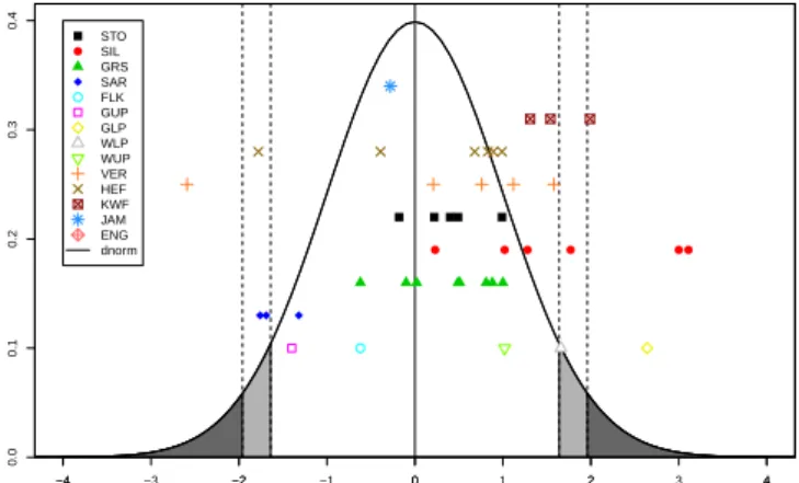
be perfectly estimated (i.e. with an infinite degree of free- dom) because most estimates of the measurement uncertain- ties result from physical approaches. The measurement dif- ference (1 PoR ) is therefore expected to follow a normal law with a variance σ common.PoR . Acceptance of H 0 is then tested whether the reduced discrepancy δ follows a centred Gaus- sion of unit variance (Fig. 4). Working with a 95 % confi- dence level (i.e. the so-called 1.96 × σ confidence interval which corresponds to the often used 2×sigma error), we can accept the hypothesis H 0 (i.e. 1 PoR = 0) if − 1.96 < δ < 1.96.
Under this condition, there is a probability of α = 5 % of making a wrong decision and rejecting H 0 although the re- sults of the two methods are actually equal (i.e. error of type I, false alarm). Alternatively using a 90 % confidence level, we can accept H 0 if − 1.64 < δ < 1.64 with a probability for an error of type I of α = 10 %. This means that mistaken re- jection of H 0 is twice as likely and more series qualify for calibration.
In search of potential systematic errors in the observations, the substantial power of the statistical test is given by the ability to reject H 0 when it is actually false and a significant difference ε really exists. If the test outcome is to accept H 0 in that case, an error of type II is therefore committed. This second type of risk, whose probability is denoted β , depends on the adopted risk α, and ε, and is given by
β = F
u α − ε σ common.PoR
− F
− u α − ε σ common.PoR
, (22) where F denotes the cumulative distribution function of the standard (zero-mean, unit-variance) normal distribution, and u α is such that F (u α ) = α. For type-I risks α of 5 % and 10 %, u α equals 1.96 and 1.64, respectively. Under higher type-I risk α (more series being flagged for calibration), the risk β of maintaining an incorrect glaciological series (not to recalibrate when the series is actually erroneous) is nat- urally expected to decrease. This second type error risk can be calculated for each mass balance series, assuming that the discrepancy ε corresponds to the measured difference 1 PoR . When the common variance of both methods is given, it is possible to estimate the lowest bias ε limit which is detectable.
This detection limit can be calculated as ε limit.PoR = u 1−α/2 + u 1−β q
σ glac.PoR 2 + σ geod.PoR 2 , (23) where again u γ is given by the cumulative distribution func- tion of the standard normal distribution as F (u γ ) = γ. For α = β = 10 % admissible errors, (u 1−α/2 + u 1−β ) is equal to 2.9, so that the detectable error is a little less than 3 times the common variance.
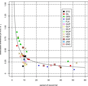
Adapting Eq. (23) for annual values of random errors for the glaciological balances (cf. Eq. 11) indicates how the threshold of difference detection is lowered for longer time series. Hence, Eq. (23) becomes
ε limit.PoR = u 1−α/2 + u 1−β q
N σ glac.a 2 + σ geod.PoR 2 (24)
so that the detectable annual difference ε limit.a is given by
ε
limit.a= ε
limit.PoRN = u
1−α/2+ u
1−βs σ
glac.a2N + σ
geod.PoR2N
2. (25) Since the uncertainty over the period of record in the geodetic balance and the annual uncertainty in the glaciological bal- ance do not depend on N, the detectable systematic error is lowered as the period of record increases, and it decreases as 1/
√
N for long time series (see Fig. 5) as 1/N 1/N 2 when N tends to large values under the square root of Eq. (25).
Calculation examples for Eqs. (19)–(25) are given in Sup- plement C.
3.5 Iteration
Once a systematic difference between the two methods is de- tected with high confidence, a first step is to locate the cor- responding error source by going back to the homogeniza- tion process and/or the uncertainty assessment. The statisti- cal exercise above thus helps to identify the survey period with the greatest discrepancies. Re-evaluating the available meta-data for each potential source of error might raise is- sues which were not considered in the first round and might lead to a new homogenization effort for one or both methods.
Re-evaluating the uncertainty assessment might reveal that uncertainties were over- or underestimated, or were not con- sidered. However, any homogenization of the observations should be well supported by measurements or process under- standing and not just for enforcing a match of the observa- tions. Unexplained discrepancies require calibration and fur- ther research.
3.6 Calibration
Calibration can be defined as the adjustment of a data series to independent observations (cf. Rykiel, 1996). If a signifi- cant difference cannot be reduced with available (meta-)data and methods in the steps above, one can take the decision to calibrate the glaciological balances – which are most sensi- tive to systematic error accumulation because of the annual observation intervals and the spatial integration issue – with the geodetic results. The aim of the calibration is to maintain the relative seasonal/annual variability of the glaciological method while adjusting to the absolute (multi-annual) values of the geodetic method. Procedures for calibration of mass balance series are described by Thibert and Vincent (2009) and by Huss et al. (2009) using statistical variance analysis and distributed mass balance modelling, respectively. Here we propose a simple approach without invoking the statis- tical linear model by Lliboutry (1974) or its expansion to unsteady state climate conditions (Eckert et al., 2011) and without the need for a numerical mass balance model.
Unless there is a clear hint of the origin of the difference,
the divergence from the geodetic balance is corrected in a
first step by calibrating the annual glaciological balances as follows.
Over a balance period of N years, for which both glacio- logical and geodetic balances are available and homoge- nized, we calculate the mean annual glaciological balance B glac.corr.a (see Eq. 15).
For each year t of the balance period, the centred glacio- logical balance β t is calculated as the deviation from the mean:
β t =B glac.corr.a.t − B glac.corr.a . (26) Over the entire balance period it results that
X N
t=1 β t = 0. (27)
Over the same balance period, the mean annual geodetic bal- ance B geod.corr.a is calculated (see Eq. 17).
For each year of the balance period, the calibrated annual balance B cal.t is defined as
B cal.t = β t + B geod.corr.a , (28)
in which the mean comes from the geodetic and the year-to- year deviation from the glaciological balance.
For any year n within the balance period, the cumulative calibrated balance is
B cal.n = X n
t=1 B cal.t = n · B geod.corr.a + X n
t =1 β t . (29)
For the last year of the balance period (n = N ), the cumu- lative calibrated balance equals the product of N times the corrected annual geodetic balance because the last term of Eq. (29) sums to 0 due to Eq. (27).
In a second step, the seasonal balances are calibrated. Un- less there is a clear hint to a bias in the spring observations, the winter balance B w remains untouched as it is usually in- dependent from the annual survey
B cal.w = B glac.w , (30)
and the difference in the annual balance B a is fully assigned to the summer balance B s as
B cal.s = B cal.a − B cal.w . (31)
Note that this does not imply that the summer balance is more prone to systematic errors than the winter balance. The pro- posed approach attributes the difference by default to the an- nual observations and leaves the winter balance untouched.
The summer balance, in most cases, is not directly measured but calculated from annual and spring observations.
Thirdly, the balances of the elevation bands are adjusted to fit the calibrated annual (or seasonal) values. For each el- evation band e of each year t of the balance period, the cen- tred elevation band balance β e.t is calculated as the deviation from the un-calibrated annual glaciological balance:
β e.t = B glac.e.t − B glac.corr.a.t . (32)
Then, the calibrated elevation band balance is defined as
B cal.e.t = β e.t + B cal.t . (33)
This approach basically shifts the glaciological balance pro- file (i.e. balance versus elevation) to fit the calibrated specific balance and, hence, maintains the balance gradient as long as the resolution of the elevation bins is high enough.
Finally, new values for ELA and AAR can be derived conventionally from the calibrated balances of the elevation bands, i.e. by fitting a curve to the calibrated surface bal- ance data as a function of altitude (cf. Cogley et al., 2011).
Note that this approach does not require changing directly observed (end-of-summer) snowlines, which are often used as (annual) equilibrium line for mass balance calculations at glaciers where all mass exchange is expected to occur at the glacier surface and with no superimposed ice. In fact, devia- tions of the calibrated ELA (and corresponding AAR) from the spatially averaged altitude of the observed snowline (and the topographic AAR) might help identifying remaining er- ror sources in the glaciological method.
Reanalysed mass balance series and derived parameters need to be flagged accordingly in any databases in which they are stored. This can be done by linking both glaciolog- ical and geodetic mass balance series through a lookup ta- ble including information on the reanalysing status (e.g. not reanalysed, homogenized only, validated but no calibration needed, validated and calibrated) and providing reference to related publications.
The calibration of glaciological mass balance series im- plies a difference of an unknown origin which might change over time (e.g. when a polythermal glacier becomes temper- ate). Note that the approach proposed here does not change the original stake and pit measurements and snowline obser- vations but fits the glacier-wide results to the geodetic bal- ance (see Sect. 5.2). This allows for reproducibility, later re- analysing exercises when new information about potential error sources or a new geodetic DEM becomes available, and/or application of statistical treatments (e.g. Lliboutry’s variance analysis model).
4 Selected glaciers with long-term observation programmes
The following analysis in Sect. 5 is based on selected glaciers with long-term measurements including both glaciological and geodetic surveys and with available information for esti- mating related uncertainties. In general, the reanalysing steps were carried out according to the best practice, as explained in Sects. 2 and 3, with individual deviations where more/less information was available for a more/less sophisticated ap- proach.
An overview of the glaciers and balance periods used
is provided in Table 1. The analysed dataset consists of
a total of 46 balance periods from 12 glaciers, including
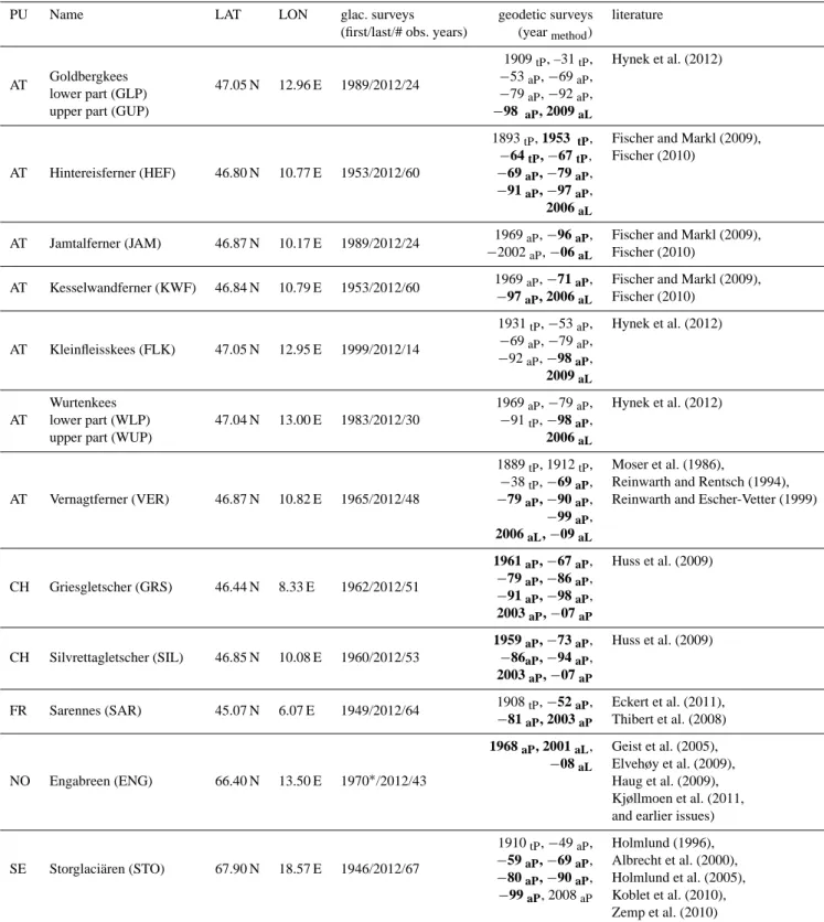
Table 1. Overview of glaciers used in this study with information about glaciological and geodetic surveys. Analysed periods of record are indicated by highlighting years of corresponding geodetic survey in bold. Methods are abbreviated as follows: t = terrestrial, a = airborne, T = tachymetry, P = photogrammetry, L = laser scanning.
PU Name LAT LON glac. surveys geodetic surveys literature
(first/last/# obs. years) (year
method)
AT 47.05 N 12.96 E 1989/2012/24
1909
tP, –31
tP, Hynek et al. (2012)
Goldbergkees − 53
aP, − 69
aP,
lower part (GLP) − 79
aP, − 92
aP,
upper part (GUP) − 98
aP, 2009
aLAT Hintereisferner (HEF) 46.80 N 10.77 E 1953/2012/60
1893
tP, 1953
tP, Fischer and Markl (2009),
− 64
tP, − 67
tP, Fischer (2010)
− 69
aP, − 79
aP,
−91
aP, −97
aP, 2006
aLAT Jamtalferner (JAM) 46.87 N 10.17 E 1989/2012/24 1969
aP, − 96
aP, Fischer and Markl (2009),
−2002
aP, −06
aLFischer (2010)
AT Kesselwandferner (KWF) 46.84 N 10.79 E 1953/2012/60 1969
aP, − 71
aP, Fischer and Markl (2009),
− 97
aP, 2006
aLFischer (2010)
AT Kleinfleisskees (FLK) 47.05 N 12.95 E 1999/2012/14
1931
tP, −53
aP, Hynek et al. (2012)
− 69
aP, − 79
aP,
− 92
aP, − 98
aP, 2009
aLAT
Wurtenkees
47.04 N 13.00 E 1983/2012/30
1969
aP, − 79
aP, Hynek et al. (2012)
lower part (WLP) − 91
tP, − 98
aP,
upper part (WUP) 2006
aLAT Vernagtferner (VER) 46.87 N 10.82 E 1965/2012/48
1889
tP, 1912
tP, Moser et al. (1986),
− 38
tP, − 69
aP, Reinwarth and Rentsch (1994),
− 79
aP, − 90
aP, Reinwarth and Escher-Vetter (1999)
− 99
aP, 2006
aL, −09
aLCH Griesgletscher (GRS) 46.44 N 8.33 E 1962/2012/51
1961
aP, − 67
aP, Huss et al. (2009)
− 79
aP, − 86
aP,
−91
aP, −98
aP, 2003
aP, − 07
aPCH Silvrettagletscher (SIL) 46.85 N 10.08 E 1960/2012/53
1959
aP, − 73
aP, Huss et al. (2009)
− 86
aP, − 94
aP, 2003
aP, −07
aPFR Sarennes (SAR) 45.07 N 6.07 E 1949/2012/64 1908
tP, − 52
aP, Eckert et al. (2011),
− 81
aP, 2003
aPThibert et al. (2008)
NO Engabreen (ENG) 66.40 N 13.50 E 1970
∗/2012/43
1968
aP, 2001
aL, Geist et al. (2005),
− 08
aLElvehøy et al. (2009), Haug et al. (2009), Kjøllmoen et al. (2011, and earlier issues)
SE Storglaci¨aren (STO) 67.90 N 18.57 E 1946/2012/67
1910
tP, − 49
aP, Holmlund (1996),
− 59
aP, − 69
aP, Albrecht et al. (2000),
−80
aP, −90
aP, Holmlund et al. (2005),
− 99
aP, 2008
aPKoblet et al. (2010), Zemp et al. (2010)
∗At ENG, the glaciological observations started one year after the first geodetic survey. The corresponding difference in time system (cf. Sect. 2.4) was accounted for using a positive degree-day model.
38 multi-annual periods with an average time span of 11 yr (ranging from 4 to 32 yr), 8 overall periods for glaciers with more than one balance period, and additional 9 balance pe- riods with alternative calculations for the example glacier Storglaci¨aren (cf. Sect. 5.1). Lower and upper parts of Gold- bergkees and Wurtenkees are analysed separately due to the disintegration of the glacier before the analysed balance peri- ods (1998–2009 and 1998–2006). Details about glaciological and geodetic surveys and related uncertainty assessments are found within the publications listed in Table 1. All glaciolog- ical and most geodetic mass balance results are made avail- able through the World Glacier Monitoring Service and pub- lished in WGMS (2012, and earlier volumes).
5 Results and discussion
5.1 Reanalysing glacier mass balance series: the example of Storglaci¨aren
Glaciological mass balance measurements on Storglaci¨aren have been carried out without interruption since 1945/1946 together with aerial surveys at approximately decadal in- tervals (Holmlund et al., 2005). The resulting vertical pho- tographs have been used to produce topographic maps, which are described in detail by Holmlund (1996). However, the volume change assessment derived from digitizing these maps has been challenged by inaccuracies in the maps and methodologies, which revealed large discrepancies as com- pared to the glaciological balances over the same periods (Albrecht et al., 2000). Koblet et al. (2010) reprocessed di- apositives of the original aerial photographs and produced a homogenized dataset of DEMs and a related uncertainty estimate. Based on these new DEMs, Zemp et al. (2010) re- analysed the glaciological and geodetic mass balance series of Storglaci¨aren, including a detailed uncertainty assessment.
Their main conclusions were that both the new geodetic and the glaciological balances (between 1959 and 1999) fit well as long as systematic corrections for internal accumulation, as proposed by Schneider and Jansson (2004), are ignored.
The conceptual framework introduced above for reanalysing mass balance series now allows these conclusions to be re- produced and quantified.
The parameters required for a statistical decision in the event that the cumulative glaciological balance significantly differs from the geodetic balance (i.e. rejection of H 0 ) are shown in Table 2, as explained in Sect. 3.4. For each balance period, the cumulative glaciological balance is corrected for systematic errors as well as for generic differences from the geodetic balance and given together with the random uncer- tainties. The geodetic balances, also corrected for systematic errors, are given with their random uncertainties. The cumu- lative discrepancy shows the difference between the two bal- ances and is put into context with the random uncertainties (through the common variance). This results in the reduced
discrepancy that allows statistical quantification of whether the two balances fit or not, as shown in the following exam- ples.
The results including the old DEMs (from Albrecht et al., 2000) for the periods 1969–1980 and 1980–1990 both have reduced discrepancies far beyond the 90 % and 95 % confi- dence levels and, hence, show that the glaciological are sig- nificantly different from the geodetic balances (i.e. H 0 to be rejected). Interestingly, there is no such discrepancy for the overall balance period (1959–1990). This is because the two strongly erroneous decades have cumulated discrepancies of opposite signs most probably caused by errors in the map of the 1980 survey. This nicely demonstrates the importance of testing both the entire balance period and the individual (multi-annual) intervals. In such a case, there are two op- tions: identify the error source in another iteration of the re- analysing process or calibrate the glaciological balance over the two balance periods with significant differences to the geodetic balances.
Koblet et al. (2010) chose the first option and homoge- nized all DEMs. Comparing these new geodetic results with the glaciological findings shows the improvements in the pe- riods 1969–1980 and 1980–1990 with much smaller cumu- lated discrepancies. H 0 is now clearly accepted for both peri- ods. However, the additional balance period (1990–99) re- veals significant differences between the methods in spite of a cumulated discrepancy similar to those of the other ac- cepted periods. Here, the reason is the better quality of DEMs which results in smaller uncertainties (i.e. a smaller common variance) and, hence, allows for an improved detection of a systematic difference.
For the same dataset (using the DEMs from Koblet et al.,
2010), the entire period of record (1959–1999) shows a large
cumulated discrepancy of more than 3 m w.e. As a conse-
quence, H 0 is to be accepted at the 95 % but to be rejected at
the 90 % confidence level. After checking all assumptions of
the uncertainty assessment, the reason is most probably to be
found in the above-mentioned over-estimation of the internal
accumulation. This is also indicated by the fact that for all pe-
riods, the reduced discrepancies are positive, i.e. the geode-
tic results are more negative than the glaciological ones. The
correction applied here for internal accumulation (i.e. 3–5 %
of the annual accumulation) is based on estimates by Schnei-
der and Jansson (2004) of re-freezing of percolation water in
cold snow and firn as well as of the freezing of water trapped
by capillary actions in snow and firn by the winter cold, based
on data from 1997/1998 and 1998/1999. Reijmer and Hock
(2008) find the internal accumulation to amount to as much
as 20 % of the winter accumulation in 1998/99 based on a
snow model coupled to a distributed energy- and mass bal-
ance model. Our comparison with the geodetic method indi-
cates that these estimates might be valid for the investigated
periods but – applied as a general correction to all years –
seem to exaggerate the contribution of the internal accumu-
lation to the annual balance.
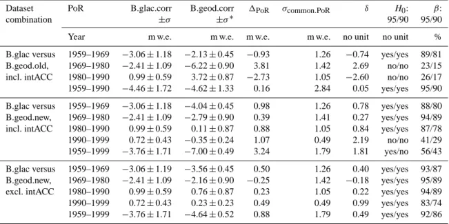
Table 2. Summary statistics for the comparison of glaciological and geodetic balances of Storglaci¨aren, Sweden. For different dataset combinations, the table shows analysed periods of record (PoR) with bias-corrected balances (B.corr) and related random uncertainties ( ± σ ) for both the glaciological (glac) and the geodetic (geod) methods, together with cumulated discrepancies (1 PoR ), common variance (σ common.PoR ), and reduced discrepancy (δ) calculated according to Eqs. (19)–(21). The acceptance (rejection) of the hypothesis (H 0 : the two balances are equal) is evaluated on the 95 % and 90 % confidence level (i.e. a type-I risk), which corresponds to reduced discrepancies inside (outside) the ± 1.96 and ± 1.64 range, respectively. For the same confidence levels, the type-II risk β (cf. Eq. 22) of not detecting an erroneous series is also given.
Dataset PoR B.glac.corr B.geod.corr 1 PoR σ common.PoR δ H 0 : β:
combination ± σ ± σ ∗ 95/90 95/90
Year m w.e. m w.e. m w.e. m w.e. no unit no unit %
B.glac versus 1959–1969 − 3.06 ± 1.18 − 2.13 ± 0.45 − 0.93 1.26 − 0.74 yes/yes 89/81 B.geod.old, 1969–1980 − 2.41 ± 1.09 − 6.22 ± 0.90 3.81 1.42 2.69 no/no 23/15 incl. intACC 1980–1990 0.99 ± 0.59 3.72± 0.87 −2.73 1.05 −2.60 no/no 26/17 1959–1990 − 4.46 ± 1.72 − 4.62 ± 1.33 0.16 2.84 0.05 yes/yes 95/90 B.glac versus 1959–1969 −3.06 ± 1.18 −4.04± 0.45 0.98 1.26 0.78 yes/yes 88/80 B.geod.new, 1969–1980 − 2.41 ± 1.09 − 2.79 ± 0.90 0.39 1.41 0.27 yes/yes 94/89 incl. intACC 1980–1990 0.99 ± 0.59 0.11± 0.87 0.88 1.05 0.84 yes/yes 87/78
1990–1999 0.72 ± 0.43 − 0.35 ± 0.24 1.07 0.49 2.19 no/no 41/29
1959–1999 − 3.76 ± 1.71 − 7.00 ± 0.49 3.24 1.79 1.81 yes/no 56/43 B.glac versus 1959–1969 − 3.06 ± 1.19 − 3.56 ± 0.45 0.50 1.26 0.40 yes/yes 93/87 B.geod.new, 1969–1980 − 2.41 ± 1.09 − 2.16 ± 0.90 − 0.25 1.42 − 0.18 yes/yes 95/89 excl. intACC 1980–1990 0.99 ± 0.59 0.76 ± 0.87 0.23 1.05 0.22 yes/yes 94/89
1990–1999 0.72 ± 0.43 0.23 ± 0.23 0.49 0.49 0.99 yes/yes 83/74
1959–1999 −3.76 ± 1.71 −4.64± 0.52 0.88 1.79 0.49 yes/yes 92/86
∗All random uncertainties are based on the new DEMs by Koblet et al. (2010) because the old ones by Albrecht et al. (2000) did not include terrain outside the glacier.
Finally, the results of the new DEMs (from Koblet et al., 2010) compared with the glaciological balances ex- cluding corrections for internal accumulation show the best fit with smallest cumulated and reduced discrepancies, and clear acceptances of H 0 for all periods. As a consequence, no calibration of the glaciological balance is needed over the reanalysed period (1959–1999). However, in spite of the relatively small discrepancies between the two methods (< 0.10 m w.e. a −1 ) there still is a great risk of not detecting a remaining difference. Future research can address this by trying to reduce the errors, such as by a co-registration of the existing elevation grids to a high-precision reference DEM of a new survey.
5.2 Calibration of glacier mass balance series: the example of Silvrettagletscher
Comparison of glaciological and geodetic mass balance se- ries of Silvrettagletscher for the periods 1994–2003 and 2003–2007 indicates a significant difference beyond the un- certainties. Huss et al. (2009) homogenized the measurement series by re-calculating seasonal mass balances based on the raw data and calibrated the cumulative glaciological balance with the geodetically determined mass change. Here, an ex- ample of the calibration of the original mass balance series
for Silvrettagletscher is provided according to the theoretical framework described in Sect. 3.6.
For the two balance periods, the differences between glaciological mass balance and the geodetic surveys are con- siderable (Fig. 2a). Whereas the cumulative glaciological balance 1994–2007 is −3.09 m w.e., the geodetic mass bal- ance indicates a cumulative balance of −7.94 m w.e. over the same period. According to the statistical test (Sect. 3.4) this difference is significant at the 95 % level and H 0 is rejected.
Since the related error source could not be clearly identified and corrected, the series for the two balance periods 1994–
2003 and 2003–2007 thus need to be calibrated.
First, the centred glaciological balance β t is calculated as
the deviation from the period mean B glac.corr.a (see Eq. 26),
and β t is subsequently shifted to agree with the mean an-
nual geodetic mass balance B geod.corr.a (see Eq. 28). This re-
sults in a calibrated series that represents a conventional mass
balance covering all components of the surface balance. The
long-term changes in glacier mass are provided by the geode-
tic surveys, and the year-to-year variability of the original
series based on the direct glaciological method is preserved
(Fig. 2a). The mean annual difference between the original
glaciological and the geodetic balance is distributed equally
over all balance years between two geodetic surveys.
1994 1996 1998 2000 2002 2004 2006 2008 Year
-8 -6 -4 -2 0
Cumulative mass balance (m w.e.) Glaciological MB
Geodetic MB Calibrated MB
a
-3 -2 -1 0 1 2
Mass balance (m w.e. a-1) ELA (uncalibrated)
ELA (calibrated)
Summer balance Annual mass balance Winter balance
0.2 0.4
Area (km2) Glaciological MB
Calibrated MB
b
2500 2600 2700 2800 2900 3000 3100
Elevation (m a.s.l.)