Future changes in vegetation and ecosystem function of the Barents Region

Future changes in vegetation and ecosystem function

of the Barents Region

Annett Wolf&Terry V. Callaghan&Karin Larson

Received: 27 June 2006 / Accepted: 3 October 2007 / Published online: 12 December 2007 # Springer Science + Business Media B.V. 2007

Abstract The dynamic vegetation model (LPJ-GUESS) is used to project transient impacts of changes in climate on vegetation of the Barents Region. We incorporate additional plant functional types, i.e. shrubs and defined different types of open ground vegetation, to improve the representation of arctic vegetation in the global model. We use future climate projections as well as control climate data for 1981–2000 from a regional climate model (REMO) that assumes a development of atmospheric CO2-concentration according to the

B2-SRES scenario [IPCC, Climate Change 2001: The scientific basis. Contribution working group I to the Third assessment report of the IPCC. Cambridge University Press, Cambridge (2001)]. The model showed a generally good fit with observed data, both qualitatively when model outputs were compared to vegetation maps and quantitatively when compared with observations of biomass, NPP and LAI. The main discrepancy between the model output and observed vegetation is the overestimation of forest abundance for the northern parts of the Kola Peninsula that cannot be explained by climatic factors alone. Over the next hundred years, the model predicted an increase in boreal needle leaved evergreen forest, as extensions northwards and upwards in mountain areas, and as an increase in biomass, NPP and LAI. The model also projected that shade-intolerant broadleaved summergreen trees will be found further north and higher up in the mountain areas. Surprisingly, shrublands will decrease in extent as they are replaced by

A. Wolf

:

Department of Physical Geography and Ecosystem Analyses, Lund University, Lund, Sweden

A. Wolf (*)

Department of Environmental Science, Institute of Terrestrial Ecosystems, Universitätsstr. 16, CH-8092 Zürich, Switzerland

e-mail: annett.wolf@env.ethz.ch

A. Wolf

:

Abisko Scientific Research Station, Abisko, Sweden T. V. Callaghan

forest at their southern margins and restricted to areas high up in the mountains and to areas in northern Russia. Open ground vegetation will largely disappear in the Scandinavian mountains. Also counter-intuitively, tundra will increase in abundance due to the occupation of previously unvegetated areas in the northern part of the Barents Region. Spring greening will occur earlier and LAI will increase. Consequently, albedo will decrease both in summer and winter time, particularly in the Scandinavian mountains (by up to 18%). Although this positive feedback to climate could be offset to some extent by increased CO2drawdown from vegetation, increasing soil respiration results in NEE close

to zero, so we cannot conclude to what extent or whether the Barents Region will become a source or a sink of CO2.

1 Introduction

Northern latitudes have already experienced dramatic climate changes in the last decades (Serreze et al. 2000; Chapman and Walsh 2003; ACIA 2005) and these changes are expected to increase. Indeed, the Arctic Climate Impact Assessment (ACIA2005) predicted an increase in temperature of 1.2°C for the 2011–2030 period, 2.5°C for 2041–2060 and 3.7°C for 2071–2090 and a mean increase in precipitation by 4.3, 7.9 and 12.3% for the respective periods. Climate changes have also occurred in the Barents Region (Pfeiffer and Jacob2005; Keup-Thiel et al.2006) and the regional climate model REMO predicts further increase in temperature of 5°C and precipitation of ca. 25% by the end of the century (Keup-Thiel et al.2006) using the moderate IPCC-SRES B2 scenario (IPCC2001).

These changes in climate have already had impacts on the vegetation (Christensen et al.

2004; Høgda et al. 2002; Tucker et al. 2001; Callaghan et al. 2004; Juday et al. 2005; Malmer et al. 2005; Tømmervik et al. 2004) and ecosystem function—e.g. fluxes and

storage of carbon of the Barents Region and wider northern areas (Oechel et al. 2000; McGuire et al.2002; Nemani et al.2003; Callaghan et al.2004). Experiments that simulate future climate change also show strong responses of the vegetation (Shaver and Jonasson

1999; Dormann and Woodin2002; Van Wijk et al.2003; Walker et al.2006).

Individualistic responses for different plant types will result in changes in vegetation composition and hence in plant biodiversity (Potter et al. 1995; Cornelissen et al. 2001; Shaver and Jonasson 1999). This in its turn will have impacts on animal biodiversity (Callaghan et al. 2004), as animals depend on plants for food, shelter and habitat. With changes in vegetation and animals, there will be a strong impact on people living in the north, as they are dependent on natural resources. We therefore expect ongoing impacts on the northern economy (forestry, agriculture, reindeer herding, tourism), some of which might be detrimental while others might lead to potential opportunities (Chapin et al.2006). The changes in vegetation and ecosystems of the north have the potential to also affect people outside the northern regions because of changing feedbacks from the land surface to the atmosphere. Vegetation influences albedo, carbon fluxes and the water cycle, and therefore potentially has a great influence on both regional and global climate (Callaghan and Jonasson1995; Harding et al.2002; Bonan et al.1992; ACIA2005; Callaghan et al.

2004; IPCC2001; Chapin et al. 2005).

Predicting and visualizing these changes might help to increase public and political awareness of the problem of climate change and draw attention to the serious impacts that anthropogenic climate change is already having in the north ,, so that appropriate mitigation and adaptation strategies can be planned and implemented (Chapin et al. 2006; Arctic Climate Impact Assessment—Policy Document2004).

With the help of vegetation models, we can predict the potential impacts of future climate change on vegetation. Earlier modelling approaches applied to northern latitude vegetation used equilibrium models such as BIOME (Cramer 1997; Skre et al. 2002; Kaplan2001). They consistently predicted a northwards movement of all vegetation types, with tundra being replaced by boreal forest. However, the equilibrium models are based on the assumption that vegetation is always in equilibrium with climate change. Considering the rapidly changing climate conditions, as well as the time needed for plants to establish, grow, reproduce, disperse and die, this assumption is unlikely to be fulfilled. It is therefore important to use models that are capable of representing continuous changes in both structure and composition of the vegetation by explicitly including life cycle processes such as those listed above. These requirements are fulfilled by dynamic vegetation models which were developed using the achievements of the equilibrium models. Our aim is to investigate these transient response of vegetation, using the advanced and specifically modified dynamic vegetation model LPJ-GUESS (Smith et al.2001; Sitch et al.2007).

In this study, we used the existing modelling framework (LPJ-GUESS, Smith et al.

2001), which models the growth and distribution of plant functional types (PFTs), but the model was especially modified for northern environments, and applied to a restricted geographical region for which validation data existed for current conditions.

In this paper we apply the model to the Barents Region. About half the population living in the Arctic live in this region (ACIA 2005), which comprises northern Scandinavia, the European part of northern Russia, Novaya Zemlya, Svalbard and Franz Josef Land. This region is climatically and environmentally diverse, extending from the high Arctic and high mountains, where unvegetated land is common, to the boreal zone. Many of its people depend on natural resources such as reindeer herding, forestry and tourism. Furthermore, there is good background data for the region that facilitates the application of models. For example, the regional climate model REMO (MPI Hamburg) delivers climate data at 0.5° resolution for the Barents Region, both for a control period (1961–2004) and future prediction (2004–2099). In addition, the climate in this area is known to have changed in past decades and there have also been changes in vegetation, some of which have been related to climate changes (Malmer et al.2005; Christensen et al.2004; Tømmervik et al.2004).

In this paper we aim to answer the following questions with the help of a state-of-the-art dynamic vegetation model specifically modified and applied to the northern environment and extensively validated: In the Barents Region, (1) will vegetation change, and if so, how? (2) where will be the areas of largest change?, (3) which types of current vegetation are most vulnerable? and (4) what are the consequences of vegetation change for ecosystem function including LAI (leaf area index), albedo and NPP (net primary production)?

2 Materials and methods

2.1 The vegetation model GUESS

We used GUESS (General Ecosystem Simulator; Smith et al.2001), which combines the mechanistic representation of plant physiological and biogeochemical processes of the LPJ-DGVM (Lund-Potsdam-Jena dynamic global vegetation model; Sitch et al. 2003) with detailed representation of vegetation dynamic processes (Smith et al.2001). The growth of cohorts of PFTs is simulated in 10 independent replicated patches. A PFT is a group of

species with similar properties so that they can be regarded as functionally similar. The cohorts possess different dynamics, depending on their characteristics (e.g. biomass, age, height) and the influence of the other vegetation in the gridcell (e.g. light extinction of vegetation growing above the cohort). PFTs used here are characterised by a number of parameters controlling establishment, growth, metabolic rates and the limits of the climate space that the PFT can occupy (AppendixA).

Photosynthesis, water uptake and plant respiration are modelled as an average for each cohort at daily time steps. At a yearly time step, the resulting annual NPP is allocated to reproduction and growth, whereby allocation and growth are determined by a set of prescribed allometric relationships. The yearly leaf and root turnover as well as biomass from plant mortality is transferred to the litter pool. Litter and soil carbon dynamics follow first-order kinetics and are sensitive to temperature and soil water.

The LPJ-GUESS is fully described in Smith et al. (2001) and further details of the physiological, biophysical and biogeochemical components of the model are given by Sitch et al. (2003). The new version used in this study includes improved representation of soil hydrology, snow pack dynamics and soil–vegetation–atmosphere exchange of water, as documented by Gerten et al. (2004) and additional PFTs appropriate to northern regions (see below). In earlier studies, the model has correctly predicted the dominant PFT composition in different sites, e.g. five pristine European forests (Badeck et al. 2001), various sites across Europe (Smith et al. 2001), a site in the U.S. Great Lake Region (Hickler et al.2004), the seasonal and interannual variation in carbon and water vapour fluxes at 15 forest sites across Europe (Morales et al. 2005) and the NPP and species composition of forests in Sweden (Koca et al.2006). The closely related LPJ-DGVM has been subjected to extensive validation of variation in ecosystem carbon balance (Lucht et al.2002; Sitch et al.2003).

2.2 Parameterisation

The biological units simulated are cohorts of plant functional types (PFTs). We used the parameterisation of Koca et al. (2006) after conversion from parameterisation at the species level to PFT-level (AppendixA). The tree PFTs were: shade-tolerant boreal needle-leaved evergreen trees (TBE), intolerant boreal needle-leaved evergreen trees (IBE), shade-intolerant broadleaved summergreen (IBS), and shade-tolerant broadleaved summergreen (TBS). If trees dominate a gridcell, we describe the land cover as forest (Table1). In this study, new shrub PFTs were introduced based on Kaplan (2001), Walker (2000) and Walker et al. (2002). They represent tall shrubs, which are shrubs up to 2 m and low shrubs which are shrubs up to 0.5 m in height, and summergreen and evergreen species of both types. If shrubs dominate a gridcell it will be described as shrub lands (Table 1). Shrubs are considered to have the same features as trees, concerning photosynthesis, respiration, and water uptake. They differ from trees in the parameterisation of allometry, which regulates the growth form of the species, in light demand, growth efficiency, root distribution and longevity (AppendixA). For shrubs, the parameter (k_allom1) is smaller than for trees, to reduce crown area increment with increasing diameter, the height growth is reduced by adapting parameters regulating the height–diameter relationship (k_allom2). Maximum crown area is also reduced, as shrubs will not reach same dimensions as trees. The parameter determining the leaf area to sapwood area ratio (k_latosa) is also reduced for shrubs, compared to trees as shrubs have lower values (Jackson et al. 1999; Kolb and Sperry1999) than trees (McDowell2002). Furthermore, sapwood turnover is reduced, as

diameter growth is not as extensive as in tree PFTs. Growth efficiency mortality is lower than for trees, as shrubs can exists in areas that are not suitable for tree growth. The climatic limits of shrub types have been adapted from Kaplan (2001) and vegetation maps (Hultén and Fries1986;http://linnaeus.nrm.se/flora/).

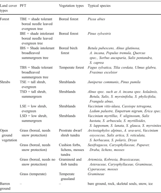
For the open ground vegetation, we considered four vegetation types; temperate grasses, graminoid and forb tundra, prostrate dwarf shrub tundra and cushion forb, lichen and moss tundra (Table1). For convenience of parameterisation, all belong conceptually to the grass life form as we do not consider them to have a height or occupy crown area. They are distinguished by their bioclimatic limits such as the amount of snow cover they require or tolerate (Kaplan2001) and the growing degree days above 0°C derived from comparison Table 1 Definition of land cover types, PFTs and vegetation types; giving examples of typical species Land cover

types

PFT Vegetation types Typical species

Forest TBE = shade tolerant

boreal needle leaved evergreen tree

Boreal forest Picea abies

IBE = shade intolerant boreal needle leaved evergreen tree

Boreal forest Pinus sylvestris

IBS = Shade intolerant broadleaved summergreen tree

Boreal birch forest

Betula pubescens, Alnus glutinosa, A. incana, Populus tremula, Quercus spec., Sorbus aucuparia, Salix pentandra, S. caprea

TBS = Shade tolerant broadleaved summergreen tree

Temperate forest Fagus sylvatica, Tilia cordata, Ulmus glabra,

Fraxinus excelsior

Shrubs TSE = tall shrub,

evergreen

Shrublands Juniperus communis, Pinus pumila

TSD = tall shrub, summergreen

Shrublands Alnus spec. such as A. incana spec. kolaänsis,

Betula, Salix, S. myrsinifolia, S. phylicifolia, Frangula alnus,

LSE = low shrub, evergreen

Shrublands Vaccinium vitis-idaea, Cassiope tetragona,

Ledum palustre, Empetrum nigrum, Erica spec. LSD = low shrub,

summergreen

Shrublands Vaccinium myrtillus, V. uliginosum, Salix

hastata, S. arbuscula, S. myrtilloides, S. lapponum, S. lanata, S. glauca, S. myrsinites Open

ground vegetation

Grass (boreal, needs snow protection)

Prostrate dwarf shrub tundra

Arctostaphylos alpinus, A. uva-ursi, Vaccinium oxycoccus, Salix artica, S. reticulata, S. herbacaea, S. polaris, Dryas Grass (boreal, needs

snow protection)

Cushion forbs, lichens, mosses tundra

Saxifragacea, Caryophyllaceae, Papaver, Draba, lichens, mosses

Grass (boreal, needs no snow protection)

Graminoid and forb tundra

Artemisia, Kobresia, Brassicaceae, Asteraceae, Caryophyllaceae, Gramineae, Cyperaceae, mosses

Grass (temperate) Temperate

grassland

Gramineae

Barren ground

with distribution maps of common species (Hultén and Fries1986;http://linnaeus.nrm.se/ flora). Table1lists typical species and the parameterisations are given in AppendixA.

2.3 Climate and CO2data

The model is driven by monthly averages of temperature, precipitation, percentage of sunshine hours, annual atmospheric CO2-concentration and soil-type derived from the FAO

global soil data set (FAO1991).

We used a 1,000 year spin-up period to allow the vegetation, soil and litter pools to reach equilibrium with the long-term climate. For this spin-up period, we used the Global Climate Dataset from the Climate Research Unit (CRU), which gridded monthly surface climate variables for the period 1901–2000, with a 0.5 degree resolution (http://ipcc-ddc.cru.uea.ac. uk/obs/cru_climatologies.html; Mitchell et al.2004). The time series from 1901–1930 was used repeatably to provide the climate input for the spin-up. For the historical period 1901– 1960 we also used data from the CRU-data set. For the period 1961–2099, we used the data from the regional climate model REMO (Jacob2001). REMO used a 0.5 degree resolution driven by ECHAM4 (Roeckner et al. 1996) data as a boundary condition. The Barents Region was laid in the centre of the regional climate model, using the grid cell coordinates from the REMO model. The climate prediction 1961–2099 was based on the SRES-B2-CO2 scenario (IPCC 2001). The CRU-point closest in distance (in longitude–latitude

degrees) to the REMO-grid point was used to derive driving data for the spin-up and 1901– 1960 periods.

Global atmospheric CO2 concentrations derived from ice-core measurements and

atmospheric observations (c.f. Sitch et al. 2003) were used for the 1901–2000 period. The CO2 concentration for the future projection is based on the SRES-B2-CO2 scenario

(IPCC2001). For the spinup period we used a constant CO2concentration of 296 ppmv

(concentration in 1901).

2.4 Map validation

As the model predicts the potential current natural vegetation of the Barents Region, two types of maps were chosen to validate the model output. Firstly, we used the map of natural vegetation in Europe (Bohn et al.2004). This map was not available as grid data and we therefore made a qualitative comparison. Secondly, we used the Olson map of global ecosystems (http://edcftp.cr.usgs.gov/pub/data/glcc/globe/latlon/goge2_0ll.img.gz; Olson

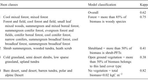
1994a,b; U.S. Geological Survey), which represents the actual vegetation of the earth as interpreted from satellite data. As the data were available on a grid base, a quantitative analysis using Kappa statistics was possible (Eklundh2003; Monserud and Leemans1992). The analysis of Olson’s Map of Global Ecosystems (U.S. Geological Survey) involved approximation of the extent of model grid cell areas, which were then overlaid with the Olson map for all modelled grid cells. We calculated an overall Kappa value and individual Kappa values for each class (Table2).

The classifications used in the maps represent ecosystem types, whereas the model predicts for trees and shrubs the biomass of plant functional types. Therefore we needed to define comparable vegetation types from our model output and to simplify the variety of ecosystem classes from the two maps. The details of classifications for the maps are shown in Tables2and Table3.To enable comparison of model output and maps, the model output, which gives the biomass for tree and shrub PFTs (kg Cm−2), was converted into vegetation types according to the rules in Tables2and3.

3 Results

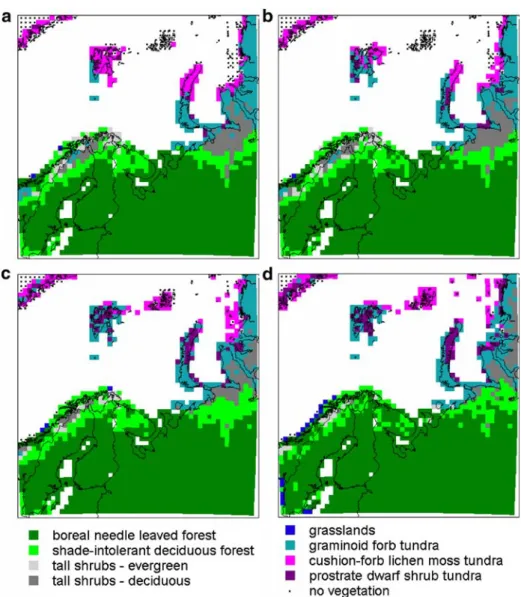
Qualitative comparison of the main vegetation types derived from the model output (Fig.1b) with the maps of natural vegetation of Europe (Bohn et al.2004; Fig.1a) showed a satisfying agreement for most of the area of the Barents Region. The vegetation associated with the Scandinavian mountains is reproduced and the birch belt along the mountain

Table 3 The simplification of the detailed map of natural vegetation (Bohn et al.2004)

Class for comparison with model

Classification according to Bohn et al.2004 Classification scheme for the model

output

Open ground vegetation

Polar deserts and subnival–nival vegetation of high mountains (Class A)

Total biomass>0.02 kgC*m−2

Arctic tundras and alpine vegetation (Class B)

Forest* More than 85% of biomass is

woody species

IBS Subarctic, boreal and nemoral–montane open

woodlands as well as subalpine and oro-Mediterranean vegetation (Class C)

More than 85% of biomass is woody species and 75% of those is IBS

BNE Mesophytic and hygromesophytic coniferous and

mixed broad-leaved-coniferous forests (Class D)

More than 85% of biomass is woody species and 75% of those is BNE

TBS Mesophytic summergreen broad-leaved and mixed

coniferous-broad-leaved forests (Class F)

More than 85% of biomass is woody species and 75% of those is TBS

wetlands Mires (Class S) Not modelled

*This class was defined for the modelling output, when forest types where not dominated by one certain PFT, but rather a mixture of different PFTs.

Table 2 Fit of the areas of modelled vegetation types compared with the Olson classification (U.S. Geological Survey)

Olson classes Model classification Kappa

Overall 0.62

1 Cool mixed forest, mixed forest Forest = more than 85% of

biomass is woody species

0.75 Forest and field, cool forest and field, small leaf

mixed woods, summergreen and mixed boreal forest, summergreen conifer forest, evergreen forest and fields, conifer boreal forest, cool conifer forest, narrow conifers, summergreen broadleaf forest, cool broadleaf forest, summergreen broadleaf forest

2 Shrub summergreen, wooded tundra, heath scrub Shrubland = more than 50% of

biomass is shrub-PFTs

0.41

3 Cold grassland, semi desert shrubs, low sparse grassland, upland tundra

Open ground vegetation = more than 50% of biomass belongs to this land cover type

0.38

4 Bare desert, sand desert, barren tundra, polar and alpine Desert

No vegetation = total

biomass<0.02 kgC m−2

0.82

The Kappa statistic was used. Kappa values vary between 0 (no fit) and 1(perfect fit), so that Kappa>0.85= excellent fit, >0.7 = very good fit, >0.55 = good fit, >0.40 = fair fit, >0.2 = poor fit (Monserud and Leemans 1992)

chains and in northern Russia is modelled satisfactory. The open ground vegetation in the northern areas is also reproduced adequately.

On the islands of the Barents Sea, the model predicted a mixture of tundra vegetation types (prostrate dwarf shrub tundra, cushion forbs, lichens and moss tundra, graminoid and

Fig. 1a Modified map of potential natural vegetation (published in agreement with BfN—Bundesamt für

Naturschutz, Germany) and b model predictions of potential natural vegetation derived from modelled

vegetation types (1981–2000). Please be aware of the slightly different projection and extent of the maps and

c major vegetation type according to Olson’s Global ecosystems map (modified, U.S. Geological Survey)

forb tundra, Table 1), which is in agreement with currently observed natural vegetation (Bohn et al.2004).

The quantitative comparison with Olson’s Global Map of Ecosystems (Olson1994a,b) showed a good agreement (Fig. 1c,d, Kappa=0.62, where a random distribution would result in a value of 0.0 degrees of agreement: after Monserud and Leemans1992).

The major disagreement between the model output and observations is in the central part of the area, at the northern Kola Peninsula and the Kanin Nos Peninsula. The model predicts predominance of boreal forest, but according to the vegetation maps (Fig. 1), the northern part of the Kola Peninsula and the Kanin Nos Peninsula should be open ground vegetation. However, total biomass is much lower (6.2 kgC m−2) than average for the boreal forests (13.1 kgC m−2) and less than half of each gridcells is forest-covered. Although the model predicts a dominance of forest, this forest is patchy, has a lower density and a lower biomass than the average predicted for boreal forest in the region.

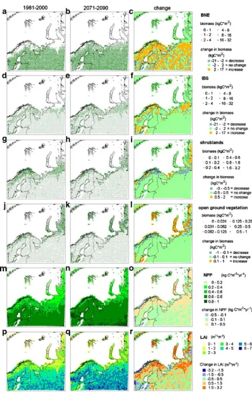
The model predictions of total biomass in BNE (13.1 kgC m−2) and IBS (5.3 kgC m−2 (Table4) are within the ranges presented by other studies of boreal forests (Table4). The model predicts a total biomass of 1.4 kgC m−2for shrublands, which is in agreement with field observations (Table4). The biomass of open ground vegetation types is also consistent with field measurements (Table4).

Both the productivity (NPP) predicted for BNE (0.65 kgC m−2yr−1) and IBS (0.49 kgC m−2yr−1) are in agreement with measurements in the field (Table4). However, shrublands have a projected productivity of 0.38 kgC m−2yr−1, which is higher than values reported from field observations (Table 4). The difference between projected and observed productivity might be explained by the mixture of high and low shrubs, and even trees, in the modelled gridcells compared with the pure shrubland patches from which observed values are derived. The productivity of temperate grassland and graminoid–forb–tundra is estimated to be 0.21 kgC m−2yr−1, which is slightly higher than observed values for total productivity. However, it lies within the range, if only aboveground productivity is considered, of total productivity. For prostrate−dwarf−shrub tundra and cushion−forb− lichen−moss tundra, the productivity predicted by the model is low and similar to observed values (Table4).

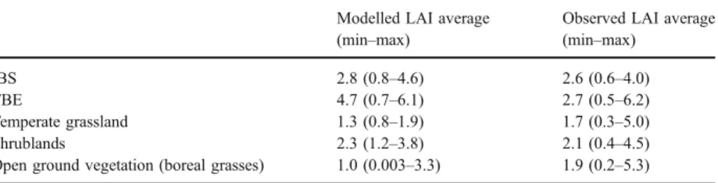
The LAI estimates from the model are generally in good agreement with the results reported by Asner et al. (2003), who published a synthesis of LAI observations (Table5). Projected LAI is consistent with observed values for shade-intolerant summergreen trees. For boreal needle leaved forests, the range of modelled values are in good agreement with the range of observed values, but the average of the modelled LAI is higher. The average values from the model for grasslands are somewhat lower than the observed average and also the maximum projected LAI for the modelled grasslands is lower than reported values. Observed grasslands also contain prairie and steppe vegetation, which have a high LAI and will therefore determine both average and maximum values for the observed data set. Good agreement with observed data is found for shrublands.

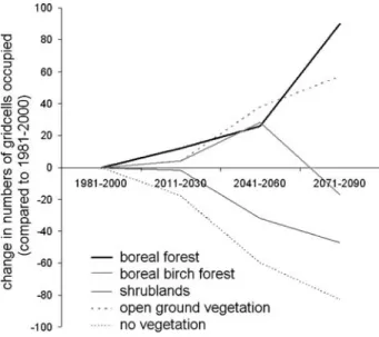
In the future, increasingly larger areas will be occupied by boreal needle leafed forest (Figs. 2, 3). Also, the area occupied by different types of open ground vegetation will increase. The two land cover types that decrease successively are the area occupied by shrubs and the presently barren land (Fig.4). Boreal birch forests (represented by the IBS PFT) show an intermediate response, with an initial increase and a following decrease. The boreal needle leafed forest PFT increases its range and successively becomes dominant in gridcells further north and at higher elevations in the mountains (Fig.2). This is a result of an increase in biomass in those gridcells, such that other PFTs are out-competed (Fig.3a–c).

T able 4 A verage, standar d dev iation (std.dev .) of total biom ass for th e main vegeta tion type s in kgC m -2 over the whole area for the 1981 –2000 modelling period Mai n veg etation T ype Modelle d total biomass ±std.dev . (kgC/m 2 ) Compa rison with measur ed values Biomass (kgC/m 2) Modelle d N PP ± std.de v (kgC/ m 2 /yr) Compa rison with measured values N P P (kgC /m 2/yr) T otal A bove ground T otal Above ground Bo real for est 13.1 ± 3.8 13 –16 a,1 5 b 4– 10 c,d,e,f 0.65 ± 0.08 0.6 b, 0.23 g,f up to 0.2 Forest dominate d b y shade-intolerant summ er green trees (birch for est) 5.3 ± 2.5 2.7 –5.0 h 3.5 f, 1.35 i, 0.32 –8.7 j 0.49 ± 0.10 0.1 1– 0.17 f,h , 0.42 j Shrubla nd 1.4 ± 0.5 1.5 k, 0.7 h, 2.35 i 0.38 ± 0.08 up to 0.16 m, usua lly lower l,h T emp erate grasslands 0.38 ± 0.29 0.38 –1.01 n 0.06 –0.48 o,p,q,r ,s,t,u,v ,w 0.14 ± 0.14 0.39 –1.24 n 0.05 –0.39 x, n Gram inoid –for b– tundra 0.35 ± 0.23 up to 0.96 y ,m,z , 0.28 –0.31 aa 0.1 –0.6 0.21 ± 0.12 0.01 –0.18 h 0.01 –0.25 m,ab, 0.04 –0.06 ac Prostra te –dw arf –shrub –tundra 0.1 1 ± 0.12 0.05 –0.19 l,h 0.06 ± 0.01 0.01 –0.07 h,l Cu shion –for b– liche n– moss –tundr a 0.01 ± 0.02 0.07 –0.4 h, 0.015 –0.4 ad , 0.16 ac 0.00 6– 0.06 ae, m,u p to 0.38 h , 0.015 –0.38 ad 0.01 ± 0.01 0.004 –0.02 7 ad 0.001 – 0.02 5 h, ad Bare grou nd 0.0 0.0 a Lehto nen et al. ( 2004 ), b Nabuurs and Schelhaa s ( 2003 ), cFa zakas et al. ( 1999 ), dLaiho and Laine ( 1997 ), eV ygodska ya et al. ( 2002 ), fV edrova ( 2002 ), g W ard le et al. ( 2003 ), h Gi lmanov and Oechel ( 1995 ), i D ahlber g ( 2001 ), jJoha nsson ( 1999 ), k Thomp son et al. ( 2004 ), l Shave r and Jona sson ( 1999 ), m Sha ver et al. ( 2001 ), n Gilmanov et al. ( 1997 ), oFrank and Duga s ( 2001 ), pBlo mqvist et al. ( 2000 ), qvan der Hoek et al. ( 2004 ), rMilne et al. ( 2002 ), sMar issink and Hans son ( 2002 ), tMuld er et al. ( 2002 ), uAustrh eim ( 2002 ), vRosset et al. ( 2001 ), wN iklaus et al. ( 2001 ), xDhillion and Gard sjord ( 2004 ), y G rogan and Jona sson ( 2003 ), z H obbie and Chapin ( 1998 ), aa Jone s and Gore ( 1981 ), ab Chapin et al. ( 1995 ), ac T ikhomirov et al. ( 1981 ), ad W ielgolaski et al. ( 1981 ), ae Press et al. ( 1998 )

BNE also invades new gridcells situated further north or higher up in the mountains and thereby increases its range.

The model predicts an increase in LAI, both in the already forested areas and in the areas of shrublands or open ground vegetation (Fig.3p–r), in the later case largely due to the

invasion of vegetation types with higher LAI. The model predicts a higher LAI in winter. This can be attributed to the northward spread of both evergreen shrubland and boreal forest, which have a higher LAI than those PFTs they displace (Fig.3). However, even in southern boreal forest, there is a predicted increase in LAI. The spring greening (increase in LAI) is predicted to be earlier and the summer maximum values of LAI higher, both in the southern areas and in the northern areas. In autumn, the total LAI will remain high for a longer time than predicted for today.

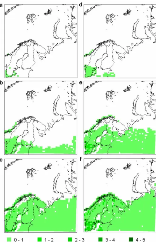
The phenological effect is strongest in summergreen trees (Fig. 5). Comparing the average LAI of summergreen trees in March, April and May predicted for the periods 1981–2000 and 2071–2090 shows that the greening front will be further north in the future. This means that there will be an earlier spring and hence an earlier leaf onset for summergreen trees. For the summergreen trees, there is no clear difference in the onset of autumn leaf fall between the periods.

The reflectivity of the vegetation, which has an important effect on energy exchange between the biosphere and atmosphere, will be reduced because of three projected trends: replacement of barren gridcells by open ground vegetation, replacement of open ground vegetation by tall shrubs and trees (Fig. 4), and an earlier spring greening. We used a correlation for northern areas between LAI and albedo or biomass and albedo (Thompson et al.2004) and estimated a decrease in albedo by an average of 4–10%. This estimation

is limited to vegetation with a biomass lower than 5 kg m−2or a LAI below 2.7 m2m−2 and therefore only valid in the most northern areas. To estimate the albedo for the whole area we used data giving summer and winter albedo for different types of vegetation (Betts and Ball 1997) and for bare soil (Oguntunde and van de Giesen 2004). We predicted an average decrease in albedo of 3% in summer and 6% in winter. In the Scandinavian mountains the changes were most dramatic with a decrease by 12% in winter and 18% in summer.

Although the model projects increases in carbon storage in phytomass, this is counteracted by a release of carbon stored in the soil. The increase of soil respiration is in the order of magnitude of the increase in NPP. The resulting NEE shows a slight source of carbon over the modelled area (NEE 0.01–0.02 kgC m−2 _yr−1_{), but this is highly}

uncertain, due to simple representation of soil processes in GUESS.

Table 5 Comparison of leaf area index (LAI: m2m−2) predicted by the model with data from a global

synthesis of leaf area index observations (Asner et al.2003)

Modelled LAI average

(min–max)

Observed LAI average

(min–max)

IBS 2.8 (0.8–4.6) 2.6 (0.6–4.0)

TBE 4.7 (0.7–6.1) 2.7 (0.5–6.2)

Temperate grassland 1.3 (0.8–1.9) 1.7 (0.3–5.0)

Shrublands 2.3 (1.2–3.8) 2.1 (0.4–4.5)

Open ground vegetation (boreal grasses) 1.0 (0.003–3.3) 1.9 (0.2–5.3)

For the model we present average values for 1981–2000, minimum (min) and maximum (max) values are

4 Discussion

We found that the model predictions of vegetation distribution are generally and qualitatively in good agreement with today’s vegetation cover depicted in maps of natural vegetation (Bohn et al.2004) and with Olson’s map of Global Ecosystem. Also, predicted biomass, LAI and NPP are in good agreement with observed data (Tables4and5). The main disagreement is found in the area of the Kola and Kanin Nos Peninsulas, where the representation of forest is overestimated, although the model projects that forest is less dense and more patchy there than in southern areas. To improve the representation of forest in this area, we tested the influence of several parameters, e.g. GDD0 (growing degree days above 0°C), GDD5

(growing degree days above 5°C), temperature extremes for the warmest and coldest month

Fig. 2 Modelled dominant vegetation types in each gridcell for the following time periods: a 1981–2000, b

Fig. 3 Change in the occupation of gridcells, presenting occupation in1981–2000, 2071–2090 and the change between the two periods: a–c boreal needle leave evergreen trees (BNE), d–f shade-intolerant

and soil moisture minimum. None of these parameters improved the prediction of forest cover in the Kola Peninsula without worsening the representation of forest at other locations in the Barents Region. This suggests that other factors limit forest distribution on the Kola Peninsula, but they are not considered in the model yet. These other factors could for example be unsuitable soil type, an excess in soil moisture with increased Sphagnum growth which creates conditions which prevent tree survival (van Breemen1995) and increases the risk of paludification (Crawford et al.2003), the presence of permafrost, climate extremes (on a daily basis), water deficits due to frozen soil water when air temperatures are suitable for photosynthesis, grazing (Helle2001; Neuvonen et al.2001; Smirnov and Sydnitsyna2003), and anthropogenic influences (Vlassova2002), although these are localised.

A potential uncertainty not explicitly considered in our model and most other ecosystem models is the migration rates of the different tree PFTs. Chapin and Starfield (1997) considered that there would be a considerable inertia in tree migration. However, trees have been observed to have migration rates of 50–200 km/100 years (Huntley 1997). In this study, the most distant gridcells occupied by forest after 100 years are 250–300 km away from currently tree-covered gridcells (gridcell midpoint to midpoint). As the migration rate predicted by the model only slightly overestimates the maximum observed migration rates, we found the modelled migration acceptable, particularly as trees often occur in small stands as outlier populations in favourable habitats beyond their main northern distribution limits in tundra vegetation and can spread quickly from such areas (Callaghan et al.2004). The model predicts vegetation composition at a scale of 0.5° longitude/ latitude, but gives no information on the detailed structure. Hence a mixed vegetation might consist of PFTs mixed within a stand or it might consist of various PFTs occurring separately as a landscape mosaic within the same gridcell. While this is a problem for interpretation of the model output, it does not interfere with the prediction of larger scale future changes.

The new explicit formulation of shrub PFTs improved the model’s capacity to predict arctic vegetation more realistically. Shrubs are an important component for structuring arctic ecosystems (Walker et al.2002; Kaplan2001) and the presence or absence of shrubs changes ecosystem function significantly (Thompson et al. 2004; McGuire et al. 2002; Chapin et al.2005).

Fig. 4 Changes over time in proportion of gridcells dominat-ed by boreal nedominat-edle leave evergreen trees (BNE), shade-intolerant summergreen trees (IBS), shrubs, open ground veg-etation (tundra/grassland) or no vegetation

Fig. 5 Average LAI (m2m-2) of summergreen trees in 1981–2000: a March, b April, c May and 2071–2090: d March, e April, f May

The use of a dynamic vegetation model enabled us to investigate the transition of vegetation in response to a changing climate. The model predicts and geographically locates and quantifies a transition from open ground vegetation (various tundra vegetation types) to shrublands, followed by the invasion of shade-intolerant summergreen trees (e.g. birch) and finally the range extension of coniferous boreal forest PFTs. The model predictions are intuitively correct and agree with observations, for example the shrub expansion into tundra areas (Sturm et al.

2001; Tape et al.2006), the increase in mountain birch forest in Scandinavia (Tømmervik et al.2004), northern forest greening and extension of the growing season (Myneni et al.1997) and increases in northern biomass (Nemani et al.2003). The model predictions, based on climate and excluding land use impacts, are also in line with our knowledge on climate-driven vegetation development after deglaciation–when tundra was replaced by shrubs, which were invaded by boreal birch forest (IBS) and finally boreal forest was established (Cox and Moore

2000; Begon et al.1996). Although this succession might not be completed within a gridcell within the time frame of a hundred years, the model predicts all the steps of the succession over the whole Barents Region, but within different gridcells.

The largest changes in vegetation are expected in the mountain areas, on the islands of the Barents Sea and in the areas where birch forest is dominating today. The mountain birch forest, represented by IBS, is predicted to move upwards in the mountains and northward replacing shrublands and open ground vegetation (tundra areas). At its southern limits, IBS is replaced by BNE. The upward movement of the treeline is in agreement with observations in Scandinavia (Sonesson and Hoogesteger1983; Kullman2002).

The model predicts a strong decline in open ground vegetation (various type of tundra) and high vulnerability within the mountain areas. In the future, barren areas and areas with sparse vegetation will diminish. As these areas are often refuges for tundra species, the vulnerability of the tundra ecosystem will further increase. On the islands of the Barents Sea and in northern Russia, the tundra is less vulnerable as there are larger areas in the north which are currently unoccupied by vegetation or only very sparsely vegetated into which tundra can relocate.

In contrast to the modelled changes that agree with changes expected from palaeo studies, succession studies, climate manipulation experiments and recently observed changes, the model surprisingly predicts a higher number of gridcells that will be occupied by tundra in the future, due to the invasion of bare soil in the north and this will lead to higher diversity and productivity in those areas. However, climate change might proceed too fast to allow all species to reach suitable areas, especially if refuge areas are situated on the isolated islands of the Barents Sea. Also, northern skeletal soils and slowly thawing ice and snow might delay the colonisation process. Also surprisingly, the model predicts that the vegetation type likely to be most vulnerable in the Barents region is shrublands as they will be replaced by forest at their southern range margins. Although there will be an increase in their northern range margins, the model predicts a lower number of gridcells dominated. This surprising (based on current observations) vulnerability of shrublands, can be partly explained by the geography of the region. Within the Barents region, there are only a few areas that shrublands can invade that will not be invaded by different forest types within the time frame of the model predictions. In other parts of the Arctic, where the distance to the coastline, which eventually limits the migration of species, is larger, the shrublands will continuously have new areas to invade over the 100 years time frame, and will not be vulnerable as predicted for the Barents Region.

The change in vegetation has important implications for feedback to the climate system. The predicted changes in PFT composition are connected with an increase in biomass, LAI

and vegetation height which agree with observations (McGuire et al.2002). This results in a decrease of albedo, which is the primary control of the energy balance between biosphere and atmosphere. An average decrease in albedo of 3% in summer and 6% in winter was predicted for the whole region, although the changes were most dramatic with a decrease by 12% in winter and 18% in summer in the Scandinavian mountains. These changes in albedo are very important for the feedback to climate as they affect heat fluxes and this will have an impact on both the microclimate and the regional climate (Harding et al. 2002; Thompson et al.2004; Bonan et al.1992; Chapin et al.2005; Beringer et al.2005). Model representation of soil processes are simplified and interpretation of results should be made with care. As changes in NEE are small compared to the changes in carbon uptake and release, uncertainties in those two processes makes predictions of NEE insecure.

The increase in LAI will change the hydrology and hence the surface runoff, which will have consequences for spring flooding, water supply during the dry season (Harding et al.

2002) and the fresh water input into the ocean. Furthermore, changes in surface hydrology and permafrost changes will affect emissions and uptake of greenhouse gases (Christensen et al. 2003; Christensen et al. 2004). Forestry and agriculture might benefit as a higher productivity is predicted for future forests (Juday et al.2005), whereas reindeer herding is likely to be negatively influenced, as there will be fewer lichens although this might be compensated by the transient increase in shrubby vegetation.

We focused in this study on the Barents Region, and have shown the importance of the specific geography there. Although similar changes such as the replacement of tundra by shrublands and the northwards and upwards movement of the tree line are expected to occur in other regions of the Arctic, the extrapolation of the results from the Barents Region to the whole Arctic should be done carefully because of the potential importance of local environmental, geographical and social factors. However, the strong changes predicted for tundra and shrub vegetation are likely to occur over most of the Arctic.

This model has improved the projections of vegetation structure in the northern latitudes by earlier models by considering the transient response of vegetation types, which makes the predictions more realistic than the earlier equilibrium models, and by modelling shrub-and open ground vegetation. The study showed also an advance on the only other regional study of the Barents Region (Cramer1997) by considering the transient response of the vegetation. An important future development for vegetation modelling is the inclusion of wetlands as a PFT and the effects of excess soil water supply on both tree and shrub growth and permafrost dynamics, as these are features generally not considered in DGVMs. Although we only used one climate change scenario, we have chosen the B2 scenario, which is moderate climatic change scenario (IPCC 2001) and it is likely, that climate change will be stronger than assumed by the B2 scenario. Therefore, the results of this study rather underestimate than overestimate the vegetation responses.

Acknowledgements The project was funded by EU grant number EVK2-2002-00169. Additional funding was provided by NCCR Climate, a research initiative of the Swiss National Science Foundation. We wish to thank people from the LPJ-GUESS modelling group at Lund University for support and inspiring discussions. We also want to thank Margareta Johansson for administrative help. We like to thank Anders Lindroth and Torben Christensen who made it possible for A. Wolf to take part in the productive atmosphere of GeoBiosphere Science Centre of Lund University.

The data of Olson’s Map of Global Ecosystems are available from U.S. Geological Survey, EROS Data

Center, Sioux Falls, SD. We thank The Federal Agency for Nature Conservation (BfN) for providing the Map of natural vegetation of Europe.

Appendix A Supporting material

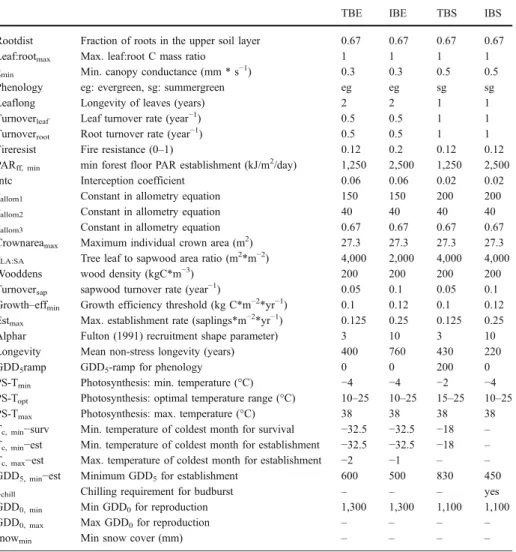
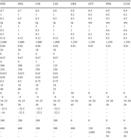
Table 6 List of parameters, which are different between PFTs and vegetation types

TBE IBE TBS IBS

Rootdist Fraction of roots in the upper soil layer 0.67 0.67 0.67 0.67

Leaf:rootmax Max. leaf:root C mass ratio 1 1 1 1

gmin Min. canopy conductance (mm * s−1) 0.3 0.3 0.5 0.5

Phenology eg: evergreen, sg: summergreen eg eg sg sg

Leaflong Longevity of leaves (years) 2 2 1 1

Turnoverleaf Leaf turnover rate (year−1) 0.5 0.5 1 1

Turnoverroot Root turnover rate (year−1) 0.5 0.5 1 1

Fireresist Fire resistance (0–1) 0.12 0.2 0.12 0.12

PARff, min min forest floor PAR establishment (kJ/m2/day) 1,250 2,500 1,250 2,500

Intc Interception coefficient 0.06 0.06 0.02 0.02

kallom1 Constant in allometry equation 150 150 200 200

kallom2 Constant in allometry equation 40 40 40 40

kallom3 Constant in allometry equation 0.67 0.67 0.67 0.67

Crownareamax Maximum individual crown area (m2) 27.3 27.3 27.3 27.3

kLA:SA Tree leaf to sapwood area ratio (m2*m−2) 4,000 2,000 4,000 4,000

Wooddens wood density (kgC*m−3) 200 200 200 200

Turnoversap sapwood turnover rate (year−1) 0.05 0.1 0.05 0.1

Growth–effmin Growth efficiency threshold (kg C*m−2*yr−1) 0.1 0.12 0.1 0.12

Estmax Max. establishment rate (saplings*m−2*yr−1) 0.125 0.25 0.125 0.25

Alphar Fulton (1991) recruitment shape parameter) 3 10 3 10

Longevity Mean non-stress longevity (years) 400 760 430 220

GDD5ramp GDD5-ramp for phenology 0 0 200 0

PS-Tmin Photosynthesis: min. temperature (°C) −4 −4 −2 −4

PS-Topt Photosynthesis: optimal temperature range (°C) 10–25 10–25 15–25 10–25

PS-Tmax Photosynthesis: max. temperature (°C) 38 38 38 38

Tc, min−surv Min. temperature of coldest month for survival −32.5 −32.5 −18 –

Tc, min−est Min. temperature of coldest month for establishment −32.5 −32.5 −18 –

Tc, max−est Max. temperature of coldest month for establishment −2 −1 – –

GDD5, min−est Minimum GDD5for establishment 600 500 830 450

kchill Chilling requirement for budburst – – – yes

GDD0, min Min GDD0for reproduction 1,300 1,300 1,100 1,100

GDD0, max Max GDD0for reproduction – – – –

References

ACIA (2005) Arctic climate impact assessment. Cambridge University Press, Cambridge, p 1042

Arctic Climate Impact Assessment—Policy Document (2004) Issued by the Fourth Arctic Council

Ministerial Meeting Reykjavik, 24 November 2004

Asner GP, Scurlock JMO, Hicke JA (2003) Global synthesis of leaf area index observations: implications for

ecological and remote sensing studies. Glob Ecol Biogeogr 12:191–205

Table 6 (continued) HSE HSS LSE LSS GRS GFT PDS CLM HSE HSS LSE LSS GRS GFT PDS CLM 0.7 0.7 0.8 0.8 0.9 0.9 0.9 0.9 1 1 1 1 0.2 0.2 0.2 0.2 0.3 0.5 0.3 0.5 0.5 0.5 0.5 0.5

eg sg eg sg sg any any any

2 1 2 1 1 1 1 1 0.5 1 0.5 1 1 1 0.6 0.6 0.5 1 0.5 1 0.5 0.5 0.5 0.5 0.12 0.12 0.12 0.12 0.5 0.5 0.5 0.5 2,000 2,000 1,000 1,000 1,250 1,250 1,250 1,250 0.06 0.02 0.06 0.02 0.01 0.01 0.01 0.01 28 30 10 10 – – – – 6 6 4 4 – – – – 0.67 0.67 0.67 0.67 _{– – – –} 4 4 1 1 – – – – 500 500 125 125 _{– – – –} 250 250 250 250 – – – – 0.015 0.015 0.01 0.01 – – – – 0.05 0.05 0.03 0.03 – – – – 0.5 0.5 0.75 0.75 – – – – 10 10 10 10 – – – – 40 40 25 25 – – – – 0 0 0 0 50 0 0 0 −4 −4 −4 −4 −4 −4 −4 −4 10–25 10–25 10–25 10–25 10–30 10–20 10–20 10–20 38 38 38 38 45 38 38 38 −32.5 −32.5 −32.5 −32.5 – – – – −16 –32.5 –32.5 –32.5 − − − − – – – – – – – – 300 200 100 100 0 0 0 0 – – – – – – – – 600 600 300 300 800 150 150 50 – – – – – 1,000 350 150 – – – – – – 50 50

TBE shade-tolerant boreal needle leaved evergreen; IBE shade-intolerant boreal needle leaved evergreen; TBS shade-tolerant broadleaved summergreen; IBS shade-intolerant broadleaved summergreen; HSW high shrub evergreen; HSS high shrub summergreen; LSE low shrub evergreen; LSS low shrub summergreen; GRS temperate grasses; GFT graminoids and forbs; CLM cushion forb, lichen and moss tundra; PDS prostrate dwarf shrubs

Austrheim G (2002) Plant diversity patterns in semi-natural grasslands along an elevational gradient in

southern Norway. Plant Ecol 161:193–205

Badeck F-W, Lischke H, Bugmann H et al (2001) Tree species composition in European pristine forests:

comparison of stand data to model predictions. Clim Change 51:307–347

Begon M, Harper JL, Townsend CR (1996) Ecology. Blackwell Science, Oxford

Beringer J, Chapin FS, Thompson CC, McGuire AD (2005) Surface energy exchanges along a tundra–forest

transition and feedbacks to climate. Agric For Meteorol 131:143–161

Betts A, Ball JH (1997) Albedo over the boreal forest. J Geophys Res 102:28901–28909

Blomqvist MM, Olff H, Blaauw MB, Bongers T, van der Putten WH (2000) Interactions between above- and belowground biota: importance for small-scale vegetation mosaics in a grassland ecosystem. Oikos 90:582–598

Bohn U, Gollub G, Hettwer C, Neuhäuslova Z, Raus T, Schlüter H, Weber H (2004) Map of the natural vegetation of Europe (Karte der natürlichen vegetation Europas). CD-ROM. Bundesamt für Naturschutz, Germany

Bonan GB, Pollard D, Thompson SL (1992) Effects of boreal forest vegetation on global climate. Nature

359:716–718

Callaghan TV, Jonasson S (1995) Arctic terrestrial ecosystems and environmental change. Phil Trans R Soc

Lond A 352:259–274

Callaghan TV, Björn LO, Chernov Y et al (2004) Climate change and UV-B impacts on arctic tundra and

polar desert ecosystems. Ambio 33(Special Issue 7):385–479

Chapin FS, Starfield, AM (1997) Time lags and novel ecosystems in response to transient climate change in

arctic Alaska. Clim Change 35:449–461

Chapin FS III, Shaver GR, Giblin AE, Nadelhoffer KJ, Laundre JA (1995) Responses of arctic tundra to

experimental and observed changes in climate. Ecology 76:694–711

Chapin FS III, Sturm M, Serreze MC et al (2005) Role of land–surface changes in arctic summer warming.

Science 310:657–660

Chapin FS III, Hoel M, Carpenter SR et al (2006) Building resilience to manage arctic change. Ambio 35

(4):198–202

Chapman WL, Walsh JE (2003) Observed climate change in the Arctic, updated from Chapman and Walsh,

1993: recent variations of sea ice and air temperatures in high latitudes. Bull Am Meteorol Soc 74:33–47

Christensen TR, Panikov N, Mastepanov M, Joabsson A, Öquist M, Sommerkorn M, Reynaud S, Svensson

B (2003) Biotic controls on CO2 and CH4 exchange in wetlands—a closed environment study.

Biogeochemistry 64:337–354

Christensen TR, Johansson T, Åkerman JH, Mastepanov M, Malmer N, Friborg T, Crill P, Svensson BH (2004) Thawing sub-arctic permafrost: effects on vegetation and methane emissions. Geophys Res Lett 31:L04501

Cornelissen JHC, Callaghan TV, Alatalo JM et al (2001) Global change and Arctic ecosystems: is lichen

decline a function of increases in vascular plant biomass? J Ecol 89:984–994

Cox CB, Moore PD (2000) Biogeography—an ecological and evolutionary approach. Blackwell Science, Oxford

Cramer W (1997) Modeling the possible impact of climate change on broad-scale vegetation structure: examples from northern Europe. In: Oechel WC, Callaghan T, Gilmanov T, Holten JI, Maxwell B, Molau U, Sveinbjörnsson B (eds) Global change and Arctic terrestrial ecosystems. Springer, New York,

pp 312–329

Crawford RMM, Jeffree CE, Rees WG (2003) Paludification and forest retreat in northern oceanic

environments. Ann Bot 91:213–226

Dahlberg U (2001) Quantification and classification of Scandinavian mountain vegetation based on field data and optical satellite images. Licentiate Thesis, Department of Forest Resource Management and Geomatics. Swedish University of Agricultural Science

Dhillion SS, Gardsjord TL (2004) Arbuscular mycorrhizas influence plant diversity, productivity, and

nutrients in boreal grasslands. Can J Bot 82:104–114

Dormann CF, Woodin SJ (2002) Climate change in the Arctic: using plant functional types in a meta-analysis

of field experiments. Funct Ecol 16:4–17

Eklundh L (2003) Geografisk informationsbehandling—Metoder och tillämpningar. Formas, Stockholm

FAO (Food and Agricultural Organisation) (1991) The digitized soil map of the World (Release 1.0). FAO, Rome

Fazakas Z, Nilsson M, Olsson H (1999) Regional forest biomass and wood volume estimation using satellite

data and ancillary data. Agric For Meteorol 98–99:417–425

Frank AB, Dugas WA (2001) Carbon dioxide fluxes over a northern, semiarid, mixed-grass prairie. Agric For

Gerten D, Schabhoff S, Haberlandt U, Lucht W, Sitch S (2004) Terrestrial vegetation and water balance—

hydrological evaluation of a dynamic global vegetation model. J Hydrol 286:249–270

Gilmanov TG, Oechel WC (1995) New estimates of organic matter reserves and net primary productivity of

the North American tundra ecosystems. J Biogeogr 22:723–741

Gilmanov TG, Parton WJ, Ojima DS (1997) Testing the‘CENTURY’ ecosystem level model on data sets

from eight grassland sites in the former USSR representing a wide climatic/soil gradient. Ecol Model

96:191–210

Grogan P, Jonasson S (2003) Controls on annual nitrogen cycling in the understorey of a sub-arctic birch

forest. Ecology 84:202–218

Harding R, Kuhry P, Christensen TR, Sykes MT, Dankers R, van der Linden S (2002) Climate feedbacks at the tundra–taiga interface. Ambio Spec Rep (Tundra–Taiga Treeline Research) 12:47–55

Helle T (2001) Mountain birch forests and reindeer husbandry. In: Wielgolaski FE (ed) Nordic mountain

birch ecosystems. The Parthenon Publishing Group, New York, pp 279–291

Hickler T, Smith B, Sykes MT, Davis MB, Sugita S, Walker K (2004) Using a generalized vegetation model

to simulate vegetation dynamics in northeastern USA. Ecology 85:519–530

Hobbie SE, Chapin FS III (1998) The response of tundra plant biomass, aboveground production, nitrogen,

and CO2 flux to experimental warming. Ecology 79:1526–1544

Høgda KA, Karlsen SR, Solheim I, Tømmervik H, Ramfjord H (2002) The start dates of birch pollen seasons

in Fennoscandia studied by NOAA AVHRR NDVI data. Proceeding of IGARSS. 24–28 June 2002,

Toronto, Ontario, Canada

Hultén E, Fries M (1986) Atlas of North European vascular plants: north of the Tropic of Cancer I–III.

Koeltz Scientific Books, Königstein

Huntley B (1997) The responses of vegetation to past and future climate changes. In: Oechel WC, Callaghan T, Gilmanov T, Holten JI, Maxwell B, Molau U, Sveinbjörnsson B (eds) Global change and Arctic

terrestrial ecosystems. Springer-Verlag, New York, pp 290–311

IPCC (2001) Climate Change 2001: The scientific basis. Contribution working group I to the Third assessment report of the IPCC. Cambridge University Press, Cambridge

Jackson GE, Irvine J, Grace J (1999) Xylem acoustic emissions and water relations of Calluna vulgaris L. at

two climatological regions of Britain. Plant Ecology 140:3–14

Jacob D (2001) A note to the simulation of the annual and inter-annual variability of the water budget over

the Baltic Sea drainage basin. Meteorol Atmos Phys 77:61–73

Johansson T (1999) Biomass equations for determining fractions of pendula and pubescent birches growing

on abandoned farmland and some practical implications. Biomass Bioenergy 16:223–238

Jones HE, Gore AJP (1981) A simulation approach to primary production. In: Bliss LC, Heal OW, Moore JJ

(eds) Tundra ecosystems: a comparative analysis. Cambridge University Press, Cambridge, pp 239–256

Juday GP, Barber B, Duffy P, Linderholm H, Rupp S, Sparrow S, Vaganov E, Yarie J (2005) Forest, land

management, and agriculture. In: ACIA, Cambridge University Press, Cambridge, pp 781–862

Kaplan J (2001) Geophysical applications of vegetation modeling. PhD thesis, Department of Plant Ecology, Lund University, Lund

Keup-Thiel E, Göttel H, Jacob D (2006) Regional climate simulations for the Barents Sea region. Boreal

Environ Res 11:1–12

Kolb TE, Sperry JS (1999) Transport constraints on water use by the Great Basin shrub Artemisia tridentata.

Plant, Cell & Environment 22:925–935

Koca D, Smith B, Sykes MT (2006) Modelling regional climate change effects on potential natural ecosystems in Sweden. Clim Change 78:381–406

Kullman L (2002) Rapid recent range-margin rise of tree and shrub species in the Swedish Scandes. J Ecol

90:68–77

Laiho R, Laine J (1997) Tree stand biomass and carbon content in an age sequence of drained pine mires in

southern Finland. For Ecol Manag 93:161−169

Lehtonen A, Mäkipää R, Heikkinen J, Sievänen R, Liski J (2004) Biomass expansion factors (BEFs) for Scots pine, Norway spruce and birch according to stand age for boreal forests. For Ecol Manag 188:211 −224

Lucht W, Prentice IC, Myneni RB et al (2002) Climatic control of the high-latitude vegetation greening trend

and Pinatubo effect. Science 296:1687–1689

Marissink M, Hansson M (2002) Floristic composition of a Swedish semi-natural grassland during six years

of elevated atmospheric CO2. J Veg Sci 13:733–742

McDowell N, Barnard H, Bond B, Hinckley T, Hubbard R, Ishii H, Köstner B, Magnani F, Marshall J, Meinzer F, Phillips N, Ryan M, Whitehead D (2002) The relationship between tree height and leaf area:

McGuire AD, Wirth C, Apps M et al (2002) Environmental variation, vegetation distribution, carbon

dynamics and water/energy exchange at high latitudes. J Veg Sci 13:301–314

Malmer N, Johansson T, Olsrud M, Christensen TR (2005) Vegetation, climatic changes and net carbon

sequestration in a North-Scandinavian subarctic mire over 30 years. Glob Chang Biol 11:1895–1909

Milne JA, Pakeman RJ, Kirkham FW, Jones IP, Hossell JE (2002) Biomass production of upland vegetation

types in England and Wales. Grass Forage Sci 57:373–388

Mitchell TD, Carter TR, Jones PD, Hulme M, New M (2004) A comprehensive set of high-resolution grids

of monthly climate for Europe and the globe: the observed record (1901–2000) and 16 scenarios (2001–

2100). July 2004. Working Paper 55. Tyndall Centre for Climate Change Research, University of East Anglia, Norwich, UK

Monserud RA, Leemans R (1992) Comparing global vegetation maps with the Kappa statistics. Ecol Model

62:275–293

Morales P, Sykes MT, Prentice CI et al (2005) Comparing and evaluating process-based ecosystem model

predictions of carbon and water fluxes in major European forest biomes. Glob Chang Biol 11:1–23

Mulder C, Jumpponen A, Högberg P, Huss-Danell K (2002) How plant diversity and legumes affect nitrogen

dynamics in experimental grassland communities. Oecologia 133:412–421

Myneni RB, Keeling CD, Tucker CJ, Asrar G, Nemani RR (1997) Increased plant growth in the northern

high latitudes from 1981–1991. Nature 386:698–702

Nabuurs GJ, Schelhaas MJ (2003) Spatial distribution of whole-tree carbon stocks and fluxes across the

forests of Europe: where are the options for bio-energy? Biomass Bioenergy 24:311–320

Nemani RR, Keeling CD, Hashimoto H, Jolly WM, Piper SC, Tucker CJ, Myneni RB, Running SW (2003) Climate-driven increases in global terrestrial net primary production from 1982 to 1999. Science

300:1560–1563

Neuvonen S, Ruohomäki K, Bylund H, Kaitaniemi P (2001) Insect herbivores and herbivory effects on mountain birch dynamics. In: Wielgolaski FE (ed) Nordic mountain birch ecosystems. The Parthenon

Publishing Group, New York, pp 207–222

Niklaus PA, Leadley PW, Schmid B, Korner C (2001) A long-term field study on biodiversity X elevated

CO2 interactions in grassland. Ecol Monogr 71:341–356

Oechel WC, Vourlitis GL, Hastings SJ, Zulueta RC, Hinzmann L, Kane D (2000) Acclimation of ecosystem

CO2 exchange in the Alaskan Arctic in response to decadal climate warming. Nature 406:978–981

Oguntunde PG, van de Giesen N (2004) Crop growth and development effects on surface albedo for maize

and cowpea fields in Ghana, West Africa. Int J Biometeorol 49:106–112

Olson, JS (1994a) Global ecosystem framework-definitions: USGS EROS Data Center Internal Report, Sioux Falls, SD, 37 p

Olson, JS (1994b) Global ecosystem framework-translation strategy: USGS EROS Data Center Internal Report, Sioux Falls, SD, p 39

Pfeiffer S, Jacob D (2005) Changes of Arctic climate under the SRES B2 scenario conditions. Meteorol Z

14:711–719

Potter JA, Press MC, Callaghan TV, Lee JA (1995) Growth responses of Polytrichum commune and

Hylocomium splendens to simulated environmental change. New Phytol 131:533–541

Press MC, Potter JA, Burke MJW, Callaghan TV, Lee J (1998) Response of a subarctic dwarf shrub heath

community to simulated environmental change. J Ecol 86:315–327

Roeckner E, Arpe K, Bengtsson L et al (1996) The atmospheric general circulation model ECHAM-4: model description and simulation of the present day climate. Max-Planck-Institut für Meteorologie Report No. 218

Rosset M, Montani M, Tanner M, Fuhrer J (2001) Effects of abandonment on the energy balance and

evapotranspiration of wet subalpine grassland. Agric Ecosyst Environ 86:277–286

Serreze MC, Walsh JE, Chapin FS III et al (2000) Observational evidence of recent change in the northern

high-latitude environment. Clim Change 46:159–207

Shaver GR, Jonasson S (1999) Response of Arctic ecosystems to climate change: results of long-term field

experiments in Sweden and Alaska. Polar Res 18:245–252

Shaver GR, Bret-Harte MS, Jones MH, Johnstone J, Gough L, Laundre J, Chapin FS III (2001) Species composition interacts with fertilizer to control long-term change in tundra productivity. Ecology

82:3163–3181

Sitch S, Smith B, Prentice IC et al (2003) Evaluation of ecosystem dynamics, plant geography and terrestrial carbon cycling in the LPJ dynamic global vegetation model. Glob Chang Biol 9:161

Sitch S, McGuire AD, Kimball J, Gedney N, Gamon J, Engstrom R, Wolf A, Zhuang Q, Clein J, McDonald KC (2007) Assessing the carbon balance of circumpolar arctic tundra using remote sensing and process

Skre OR, Baxter R, Crawford MM, Callaghan TV, Fedorkov A (2002) How will the tundra–taiga interface

respond to climate change? Ambio Spec Rep (Tundra–Taiga Treeline Research) 12:37–46

Smirnov KA, Sudnitsyna TN (2003) Changes of structural and physicochemical parameters of spruce forest

ecosystem under the effect of moose (Alces alces L.). Russ J Ecol 34:175–180

Smith B, Prentice IC, Sykes MT (2001) Representation of vegetation dynamics in the modelling of terrestrial ecosystems: comparing two contrasting approaches within European climate space. Glob Ecol Biogeogr

10:621–637

Sonesson M, Hoogesteger J (1983) Recent tree-line dynamics (Betula pubescens Ehrh. Ssp. Tortuosa (Ledb.)

Nyman) in northern Sweden. Nordicana 47:47–54

Sturm M, Racine C, Tape K (2001) Increasing shrub abundance in the Arctic. Nature 411:546–547

Tape K, Sturm M, Racine C (2006) The evidence for shrub expansion in Northern Alaska and the Pan-Arctic.

Glob Chang Biol 12:686–702

Tikhomirov BA, Shamurin VF, Aleksandrova VD (1981) Phytomass and primary production of tundra communities, USSR. In: Bliss LC, Heal OW, Moore JJ (eds) Tundra ecosystems: a comparative analysis.

Cambridge University Press, Cambridge, pp 227–238

Thompson C, Beringer J, Chapin FS III, McGuire AD (2004) Structural complexity and land-surface energy

exchange along a gradient from arctic tundra to boreal forest. J Veg Sci 15:397–406

Tømmervik H, Johansen B, Tombre I, Thannheiser D, Høgda KA, Gaare E, Wielgolaski FE (2004) Vegetation changes in the Nordic mountain birch forest: the influence of grazing and climate change.

Arct Antarct Alp Res 46:323–332

Tucker CJ, Slayback DA, Pinzon JE, Los SO, Myneni RB, Taylor MG (2001) Higher northern latitude normalized difference vegetation index and growing season trends from 1982 to 1999. Int J Biometeorol

45:184–190

van Breemen N (1995) How Sphagnum bogs down other plants. Trends Ecol Evol 10:270–275

van der Hoek D, van Mierlo AJEM, van Groenendael JM (2004) Nutrient limitation and nutrient-driven

shifts in plant species composition in a species-rich fen meadow. J Veg Sci 15:389–396

Van Wijk MT, Williams M, Laundre JA, Shaver GR (2003) Interannual variability of plant phenology in tussock tundra: modelling interactions of plant productivity, plant phenology, snowmelt and soil thaw.

Glob Chang Biol 9:743–758

Vedrova EF (2002) The carbon balance in natural and disturbed forests of the southern taiga in central

Siberia. J Veg Sci 13:341–350

Vlassova TK (2002) Human impacts on the tundra–taiga zone dynamics: the case of the Russian Lesotundra.

Ambio Spec Rep (Tundra–Taiga Treeline Research) 12:30–36

Vygodskaya NN, Schulze E-D, Tchebakova NM et al (2002) Climatic control of stand thinning in

unmanaged spruce forests of the southern taiga in European Russia. Tellus Series B 54B:443–461

Walker DA (2000) Hierarchical subdivision of Arctic tundra based on vegetation response to climate, parent

material and topography. Glob Chang Biol 6(S1):19–34

Walker DA, Gould WA, Maier HA, Raynolds MK (2002) The circumpolar Arctic vegetation map: AVHRR-derived base maps, environmental controls, and integrated mapping procedures. Int J Remote Sens

23:4551–4570

Walker MD, Wahren CH, Hollister RD et al (2006) Plant community responses to experimental warming

across the tundra biome. Proc Natl Acad Sci USA 103:1342–1346

Wardle DA, Hörnberg G, Zackrisson O, Kalela-Brundin M, Coomes DA (2003) Long-term effects of wildfire

on ecosystem properties across an island area gradient. Science 300:972–975

Wielgolaski FE, Bliss LC, Svoboda J, Doyle G (1981) Primary production of tundra. In: Bliss LC, Heal OW, Moore JJ (eds) Tundra ecosystems: a comparative analysis. Cambridge University Press, Cambridge, pp