FLIP-FLOPS AS OBSERVATIONAL SIGNATURES OF DIFFERENT DYNAMO MODES IN COOL STARS
D. M. FLURI1and S. V. BERDYUGINA1,2 1Institute of Astronomy, ETH Zentrum, 8092 Zurich, Switzerland
(e-mail: [email protected])
2Astronomy Division, University of Oulu, P.O. Box 3000, 90014 Finland
(Received 2 September 2004; accepted 29 September 2004)
Abstract. Cool, rapidly rotating stars exhibit enhanced magnetic activity with cyclic behavior on
var-ious time scales. In particular, the longitude of the dominant activity region switches quasi-periodically by 180◦, which is known as the “flip-flop” phenomenon. In the present paper we introduce a new ap-proach for the interpretation of stellar cycles based on light curve modeling with dipole and quadrupole dynamo modes. We discuss the observational signatures of different combinations of the dynamo modes. The proposed simple model is able to reproduce the basic properties of long-term photometric behavior of active stars and allows us to study different mechanisms resulting in flip-flops.
1. Introduction
Strong magnetic activity is common on cool, rapidly rotating stars. Many properties of their activity are familiar from solar physics, such as spots, enhanced X-ray emission from active regions and activity cycles. The strong activity allows to study many features in a more pronounced way than on the Sun. In addition, the large number of highly active stars gives us a large statistical sample to improve our knowledge of solar magnetic activity and its cyclic behavior.
The magnetic properties of highly active stars can be followed to a large de-gree by photometric measurements. Such stars exhibit huge spot regions that can cover easily 10 or 20% of the stellar surface (e.g., Strassmeier, 1999). Whether such regions consist of a single spot or a group of many smaller spots cannot be distinguished with current observational and theoretical methods. When such a big spot concentration passes over the visible stellar disk the luminosity is strongly reduced, typically by the order of 0.1 mag (e.g., Henry, Eaton, and Hamer, 1995). Thus, stellar spot patterns can be inferred just from photometry despite the fact that stellar surfaces are not resolved by current instruments.
Of particular interest is the observation that the biggest active regions tend to ap-pear always at similar longitudes, which are called “active longitudes.” These active longitudes are persistent over many cycles but can drift slowly due to differential rotation.
The dominant active longitude can suddenly shift by 180◦to the other side of the star, a phenomenon known as “flip-flop,” which was first observed by Jetsu et al. (1991) on FK Com. Recently, it became clear that flip-flops are rather common
ten occur with a shorter periodicity than the main activity cycle. On the Sun, for instance, they occur about every 1.8 years (Berdyugina and Usoskin, 2003).
Inspired by the results of Moss (2004) we introduce in this paper a new method to interpret stellar and solar activity based on different dynamo modes and discuss two possible mechanisms resulting in flip-flops. Starting from a given magnetic field distribution on the stellar surface we obtain many observable quantities, both photometric and polarimetric. Our method does not explain how the various dynamo modes are excited, a problem that we have omitted on purpose at this stage because of the difficulties of current dynamo models to reproduce observed data. However, our method enables an easy quantitative interpretation of stellar data and allows us to compare computed dynamo solutions with observations.
2. Modeling Stellar Activity Using Dynamo Modes
In this section we introduce how to model light curves starting from a given com-bination of dipole and quadrupole dynamo modes. The procedure consists of two steps. First, the magnetic field distribution is converted into a surface map of the irradiated intensity, which indicates the probability that spots appear at certain lo-cations. In the second step the light curve is deduced from the intensity map. This allows the study of many photometric phenomena of stellar activity. The details of the procedure and the applied assumptions are described below.
To obtain the intensity map of the stellar surface we start from a given magnetic field distribution, which can be any superposition of the four mean-field dynamo modes shown in Figure 1. This magnetic field distribution is then translated into an intensity map, following the rule that spots appear most probably at the locations of the strongest magnetic fields. Areas with zero magnetic field, indicating the quiet photosphere, are assumed to be the brightest regions. Then, the intensity is decreased proportionally to the increasing field strength, which can be understood in terms of an increasing spot filling factor. The resulting intensity map corresponds, therefore, to a probability distribution of spots. The darker the area, the larger the
Figure 1. Dipole and quadrupole dynamo modes used in this paper. The four panels show the surface
distribution of the poloidal component of the magnetic field. White and black (as the two extremes of the gray scale) indicate opposite polarities of the magnetic field. The A0 and S0 modes at the top represent two axisymmetric modes while A1 and S1 are non-axisymmetric with respect to the rotation axis (which is assumed in vertical direction).
probability that a spot appears at that location. This allows the study of global activity patterns without getting lost in modeling individual spots.
The step to obtain the intensity map from the magnetic field distribution contains the biggest assumptions in our method, but it is not so critical as it might appear at first. Clearly, spots are connected to strong magnetic fields. On the other hand, the intensity difference between spots and the photosphere is not a priori known. It can however be considered as a free parameter which can be determined from the observed light curves. Further, we neglect bright spots or faculae, which is a justified assumption for highly active stars where the cool spots dominate the long-term brightness variations (Radick et al., 1998). This is, however, in contrast to the Sun, which is brighter at activity maximum due to faculae and network.
Figure 2 shows an example of the two basic steps involved in our method. The magnetic field resulting from a superposition of the A0 and S1 modes (left panel) is transformed into the intensity map or spot probability distribution (middle panel). The light curve (right panel) is obtained from the intensity image under the assumption that the magnitude of the unspotted star is 1.1 mag and the inclination of the rotation axis to the line of sight is 60◦. The light curve has just one distinct minimum because we see more of the northern hemisphere due to the inclination.
3. Flip-Flop Mechanisms
In this section we illustrate how the various quantities, which are observed photo-metrically, can be obtained from our method. In particular, we focus on mechanisms leading to flip-flops.
correspond to the phase 0.25. The inclination is assumed to be 60 .
Flip-flops can only occur if active longitudes exist. The latter require breaking of the axial symmetry. Therefore, it is natural to introduce non-axisymmetric dynamo modes: they break the axial symmetry and also explain the concentration of active regions and spots at certain longitudes. A further requirement for getting flip-flops is time evolution of the dynamo mode configuration.
In the following we will look at two basic time dependent superpositions of the four dynamo modes introduced in Figure 1. This allows to study qualitatively two independent mechanisms leading to flip-flops.
3.1. SIGN-CHANGE OF AXISYMMETRIC MODE
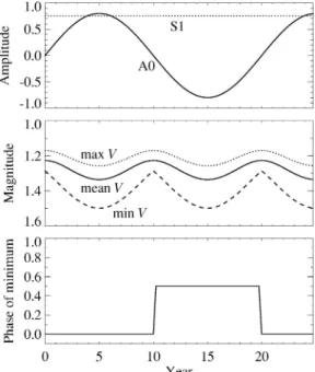
The first mechanism is based on the sign-change of an axisymmetric mode, in our example of a time dependent A0 mode. It is superposed with a constant non-axisymmetric mode S1 as plotted in the top panel of Figure 3, resulting in a tilted dipole with a periodically changing tilt angle. A similar configuration was obtained by Moss (2004) who computed a stable dynamo model with an almost constant non-axisymmetric field of mixed polarity and an oscillating axisymmetric field in which both parity and energy are strongly time-dependent.
Using the magnetic field distribution and assuming an inclination of the stel-lar rotation axis of 60◦ we compute a time series of light curves as explained in Section 2. The middle panel of Figure 3 shows the time evolution of the maximum, mean, and minimum magnitude of the light curves. They exhibit time variations with half the periodicity of the A0 mode. The maximum and minimum magni-tudes increase and decrease simultaneously, with the minimum showing stronger variations.
In this setup flip-flops occur in a natural way. The crucial point is that the A0 mode changes its sign periodically (every 10 years in our example). By changing the sign of the A0 mode, the active longitudes in both hemispheres shift suddenly by 180◦, which is nothing else than a flip-flop. If we recall that we see primarily
Figure 3. First flip-flop mechanism due to a sign-change of the axisymmetric mode A0. Input is the
time dependence of the two dynamo modes A0 and S1 (top panel). Of the resulting light curves we show the maximum, mean, and minimum value of the magnitude (middle panel). The phase of the minimum of the light curves (bottom panel) switches by 0.5 whenever the A0 mode changes the sign. We assumed an inclination of the stellar rotation axis of 60◦.
the northern hemisphere due to the inclination, it becomes obvious that the phase of the minimum of the light curve (bottom panel of Figure 3) shifts by 0.5 at the moment, when a sign-change of the A0 mode occurs. Accordingly, flip-flops and A0 sign-changes have the same frequencies, and the full flip-flop cycle has the same length as the A0 cycle. Note that at the moment of the flip-flop the light curve shows equal minima separated by 0.5 in phase due to the S1 mode. Then, spots preferably occur near the equator and the active longitudes are of opposite polarity.
In principle, we would also obtain flip-flops by keeping the A0 mode constant and by varying the sign and amplitude of the S1 mode. However, in alpha–omega dynamos, it is expected that the axisymmetric field will oscillate, whereas non-axisymmetric fields are more generally believed to be steady in some rotating frame. 3.2. ALTERNATING NON-AXISYMMETRIC MODES
In the second flip-flop mechanism we assume a superposition of dynamo modes as given in the top panel of Figure 4. The axisymmetric modes A0 and S0 remain constant while the non-axisymmetric modes A1 and S1 vary in antiphase with a period of 10 years. None of the modes ever changes its sign.
Figure 4. Second flip-flop mechanism due to varying non-axisymmetric modes in antiphase. The
three panels show the same quantities as in Figure 3. Again, we have assumed an inclination of 60◦. Flip-flops (see bottom panel) occur when different non-axisymmetric modes start to dominate.
The light curves show a completely different behavior as compared to the pre-vious example. Now, the maximum of the brightness increases when the minimum decreases and vice versa, while the mean brightness varies only slightly. Whenever the two non-axisymmetric modes A1 and S1 are of comparable strength, the light curve is almost flat. In contrast to the first mechanism, the cycle length is now in general equal to the one of the A1 and S1 modes with a strong first harmonic.
Flip-flops (see bottom panel of Figure 4) occur when the A1 and S1 modes are of equal strength. Therefore, the time between two flip-flops is not always identical and could be further modified by changing the relative strength of the A1 and S1 modes. Note that flip-flops occur without any sign-change in the dynamo modes. A more careful examination shows that this combination of dynamo modes results in polar and equatorial spots with opposite polarity, a situation often found in Doppler images. In general either the polar or equatorial spots dominate, a role which is exchanged when a flip-flop occurs. Note however that with current mean field dynamos it is seems harder to achieve this mechanism than the one discussed in Section 3.1.
4. Discussion of Activity Patterns
The long-term variations of light curves discussed in Section 3 (cf. middle panels of Figures 3 and 4) are typical for many active stars. Henry, Eaton, and Hamer
(1995) have studied active binaries and identified two types of activity patterns based on photometric data, which agree exactly with the two examples discussed in the previous section. Out of a sample of 11 active binaries he found three stars that show activity patterns corresponding to the mechanism involving an oscillating axisymmetric mode (Figure 3). More common is the second type (8 out of 11 stars) which corresponds to the pattern obtained with alternatively oscillating non-axisymmetric modes (Figure 4). This qualitative agreement shows that our method is able to reproduce realistic global activity patterns. A subsequent quantitative analysis of stellar data can result in estimates of parameters of the involved dynamo modes. This is a subject of a forthcoming paper.
It is not excluded that different combinations of dynamo modes yield similar long-term patterns of the light curves. However, our method produces many addi-tional observable quantities, such as flip-flops, polarity of the magnetic field, and the longitude and latitude of major spot concentrations. When fitting observed data, all these observables together will help to identify the magnetic field configuration.
5. Conclusions
We have introduced a new method that allows us to interpret activity patterns observed on cool stars in terms of dynamo modes and compare computed dynamo solutions with observations.
In this paper we followed the direct approach, i.e., we started from magnetic field distributions and calculated intensity maps and light curves. The method results in many observables, such as light curves, flip-flops, and the polarity and distribution of spots. We discussed two configurations of dynamo modes that reproduce two types of activity patterns commonly observed in active stars. These two config-urations naturally lead to the occurrence of flip-flops. In particular we found the possibility to get flip-flops without sign-changes in the dynamo modes. More com-plex, multi-cyclic behavior of stellar activity could for example be reproduced with a combination of the two configurations.
In the future, we intend to proceed also in the inverse direction, starting from observed light curves and inferring the intensity and magnetic field distributions. This will allow to collect quantitative information on long-term activity cycles and on the underlying superposition of dipole and quadrupole dynamo modes of many individual stars.
Acknowledgements
We thank the referee David Moss for his constructive comments helping to improve the manuscript. S.V. Berdyugina acknowledges the support by the Academy of Finland, grant No. 43039.