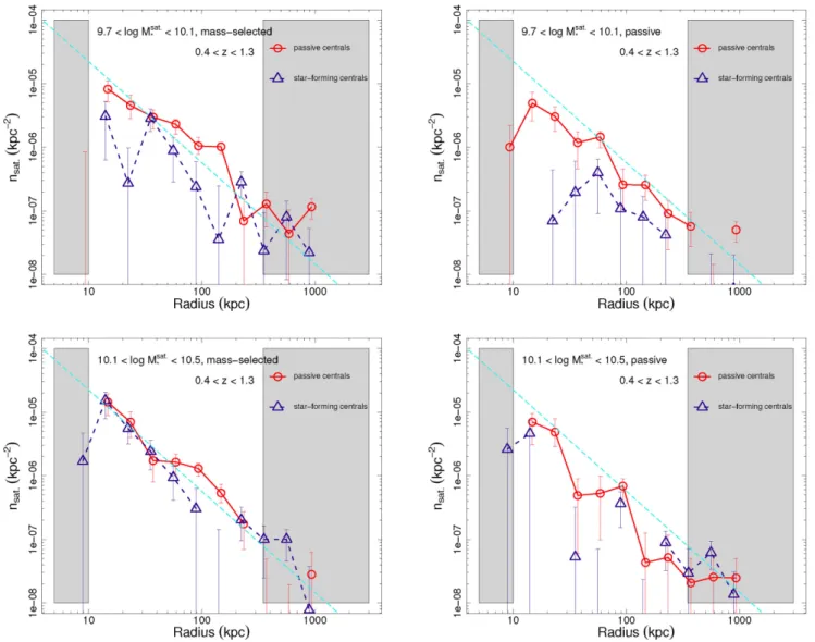
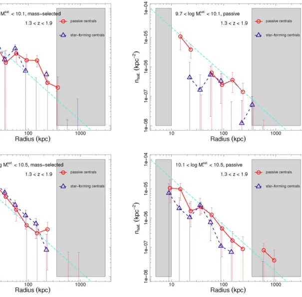
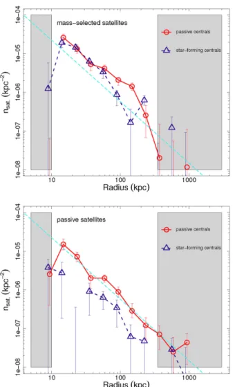
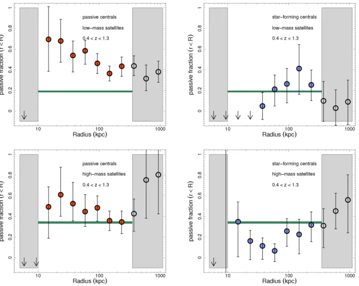
Galactic conformity and central/satellite quenching, from the satellite profiles of M* galaxies at 0.4 Hartley, W. G. ; Conselice, C. J. ; Mortlock, A. ; Foucaud, S. ; Simpson, C. In: Monthly Notices of the Royal Astronomical So

If an abstract graph G admits an edge-inserting com- binatorial decomposition, then the reconstruction of the graph from the atomic decomposition produces a set of equations and

Consequently, we try the upwind diffusive scheme associated to (1) and (7), and explain how we can obtain a good numerical approximation of the duality solution to the

Our result is also applied in order to describe the equilibrium configuration of a martensitic multistructure consisting of a wire upon a thin film with contact at the origin (see

Stochastic iterated function system, local contractivity, recurrence, invariant measure, ergodicity, random Lipschitz mappings, reflected affine stochastic recursion.. The first

Iwasawa invariants, real quadratic fields, unit groups, computation.. c 1996 American Mathematical

Then, with this Lyapunov function and some a priori estimates, we prove that the quenching rate is self-similar which is the same as the problem without the nonlocal term, except

Although the proposed LALM and LADMs are not necessarily always the fastest (again, for matrix completion problems with small sample ratios relative to rank(X ∗ ), the APGL

This result improves the previous one obtained in [44], which gave the convergence rate O(N −1/2 ) assuming i.i.d. Introduction and main results. Sample covariance matrices