Combating fake news with adversarial domain adaptation and neural models

Combating Fake News with Adversarial Domain

Adaptation and Neural Models

by

Brian Xu

B.S., Massachusetts Institute of Technology (2018)

Submitted to the Department of Electrical Engineering and Computer

Science

in partial fulfillment of the requirements for the degree of

Master of Computer Science and Engineering

at the

MASSACHUSETTS INSTITUTE OF TECHNOLOGY

February 2019

c

○ Massachusetts Institute of Technology 2019. All rights reserved.

Author . . . .

Department of Electrical Engineering and Computer Science

February 1, 2019

Certified by . . . .

James R. Glass

Senior Research Scientist

Thesis Supervisor

Certified by . . . .

Mitra Mohtarami

Research Scientist

Thesis Supervisor

Accepted by . . . .

Katrina LaCurts

Chair, Master of Engineering Thesis Committee

Combating Fake News with Adversarial Domain Adaptation

and Neural Models

by

Brian Xu

Submitted to the Department of Electrical Engineering and Computer Science on February 1, 2019, in partial fulfillment of the

requirements for the degree of

Master of Computer Science and Engineering

Abstract

Factually incorrect claims on the web and in social media can cause considerable damage to individuals and societies by misleading them. As we enter an era where it is easier than ever to disseminate “fake news” and other dubious claims, automatic fact checking becomes an essential tool to help people discern fact from fiction. In this thesis, we focus on two main tasks: fact checking which involves classifying an input claim with respect to its veracity, and stance detection which involves determining the perspective of a document with respect to a claim. For the fact checking task, we present Bidirectional Long Short Term Memory (Bi-LSTM) and Convolutional Neural Network (CNN) based models and conduct our experiments on the LIAR dataset [Wang, 2017], a recently released fact checking task. Our model outperforms the state of the art baseline on this dataset. For the stance detection task, we present bag of words (BOW) and CNN based models in hierarchy schemes. These architec-tures are then supplemented with an adversarial domain adaptation technique, which helps the models overcome dataset size limitations. We test the performance of these models by using the Fake News Challenge (FNC) [Pomerleau and Rao, 2017], the Fact Extraction and VERification (FEVER) [Thorne et al., 2018], and the Stanford Natural Language Inference (SNLI) [Bowman et al., 2015] datasets. Our experiments yielded a model which has state of the art performance on FNC target data by using FEVER source data coupled with adversarial domain adaptation [Xu et al., 2018].

Thesis Supervisor: James R. Glass Title: Senior Research Scientist Thesis Supervisor: Mitra Mohtarami Title: Research Scientist

Acknowledgments

I would like to thank my thesis advisors Mitra Mohtarami and James Glass for their efforts in guiding and assisting with my research. Without their efforts, my thesis would not have been possible. I would also like to thank all of my friends and family for their unwavering love and support throughout my academic journey.

Contents

2.3 Adversarial Domain Adaptation . . . 26

3 The Fact Checking Problem 29 3.1 Dataset Description . . . 29

3.2 Method . . . 32

3.2.1 CNN Architecture . . . 32

3.2.2 Bi-LSTM Architecture . . . 33

3.2.3 Stacked LSTM and CNN Model Architecture . . . 33

3.2.4 Evaluation Metrics . . . 34

3.3 Experiments . . . 35

3.3.1 CNN Experiments . . . 36

3.3.2 Bidirectional LSTM Experiments . . . 37

3.3.3 Stacked Bidirectional LSTM and CNN Experiments . . . 37

3.5 Discussion . . . 39

3.6 Summary . . . 40

4 Stance Detection using Adversarial Domain Adaptation 41 4.1 Datasets . . . 41

4.1.1 Fake News Challenge . . . 42

4.1.2 Fact Extraction and VERification . . . 43

4.1.3 Stanford Natural Language Inference . . . 45

4.2 Method . . . 46

4.2.1 Feature Extraction Component . . . 47

4.2.2 Label Prediction Component . . . 48

4.2.3 Domain Adaptation Component . . . 48

4.2.4 Model Parameters and Training Procedure . . . 49

4.3 Experiments . . . 50

4.3.1 Baselines . . . 50

4.3.2 Evaluation Metrics . . . 51

4.3.3 Model Configurations . . . 52

4.4 Results and Analysis . . . 54

4.4.1 Performance Analysis: FEVER → FNC . . . 54

4.4.2 Performance Analysis: SNLI → FNC . . . 55

4.4.3 Performance Analysis: SNLI → FEVER . . . 59

4.4.4 Performance Analysis: FNC → FEVER . . . 61

4.4.5 Training Loss Trends . . . 61

4.5 Summary . . . 62

5 Stance Detection Demonstration 65 5.1 Demonstration System Design . . . 65

5.2 An Example through the Demonstration System . . . 66

5.3 Technologies . . . 71

5.4 Extensibility . . . 71

6 Conclusion 73 6.1 Summary . . . 73 6.2 Future Work . . . 74

List of Figures

3-1 Model of a generic CNN as presented in [Kim, 2014]. The input sen-tence is first converted into a matrix of word vectors. Then, kernels of filter size 2 and 3 are applied, with multiple filters per filter size. The vectors are then pooled and the results are fully connected to a hidden layer. . . 32 3-2 Model of a generic LSTM cell as presented by Chen [Chen, 2016].

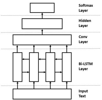
LSTM cells contain a input and output gates of a LSTM cell control information flow to and from the memory unit. Additionally, LSTM cells have a forget gate, which can be used to remove information from the memory cell. . . 34 3-3 Diagram of Bi-LSTM and CNN model. The input layer is first fed into

the Bi-LSTM layer. The features extracted from the Bi-LSTM layer are then fed into the convolutional layer. Finally, the output from the convolutional layer is fed into a fully connected hidden layer before undergoing classification via a final softmax layer. . . 35

4-1 The architecture of our model for stance detection which uses adver-sarial domain adaptation. . . 47 4-2 Exploring learning with adversarial domain adaptation across

differ-ent domains (SNLI, FEVER, and FNC datasets) and tasks (stance detection and textual inference tasks). . . 50

4-3 The classification and domain adaptation losses on validation data across training epochs for our best FEVER→FNC model; BOW + CNN + DA with the hierarchy scheme. . . 62 5-1 The high level design of the demonstration system. The client sends a

claim-document pair to the server to be analyzed. Upon receiving the request, the server processes the input texts, gives them through our pretrained stance detection model, and then returns the results. The client receives these results and displays them to the user. . . 66 5-2 The input page of the demonstration system. The user can enter two

text inputs as claim and document. Then, the inputs are processed by the demonstration system after clicking the submit button. . . 67 5-3 The first part of the results page contains a color key and statistics of

our model predictions for the input claim-document pair at a holistic level. The sentences in the document that support the predictions are highlighted. . . 68 5-4 The second part of the results page contains model predictions specific

to each sentence in the document. In particular, the specific sentence along with the claim is passed to the model and the model predictions are displayed. . . 69 5-5 This figure is in continuous of the previous part of the system outputs

List of Tables

1.1 Examples of data used for the fact checking task. . . 18

1.2 Examples of data used for the stance detection task. . . 19

3.1 Examples of claim, label pairs from the LIAR dataset. . . 30

3.2 Label frequency distribution for the LIAR dataset. . . 31

3.3 Party affiliation frequency distribution for the LIAR dataset. . . 31

3.4 Model Accuracy Results. The ’Wang’ prefix denotes results from orig-inal LIAR paper [Wang, 2017]. Suffixes subject, party, credit, and all indicate that the corresponding pieces of metadata were used. Best model was picked by choosing the highest validation accuracy model out of 10 trained. Avg indicates average accuracy over 10 trained models. 39 4.1 Randomly chosen examples of claim-document pairs and their labels from the FNC dataset. The relevant snippet from each document is displayed. . . 42

4.2 Label frequency distribution for the FNC dataset. . . 43

4.3 Randomly chosen examples of data from the FEVER dataset. The name of each document associated with the claim is given in italics, followed by the relevant snippet from the document. . . 44

4.4 Label frequency distribution for the FEVER dataset. . . 44

4.5 Randomly chosen examples of data from the SNLI dataset. The premise-hypothesis pairs are considered as the claim-document pairs. . . 45

4.7 FEVER → FNC. Results on the FNC test data for models trained using FNC training data and FEVER data. BOW, CNN and DA refer to our model when it uses bag of words features, convolutional features, and domain adaptation, respectively. When DA is present, square brackets indicate which features are passed to the domain adaptation component. The hierarchy in parentheses refers to our model with two level prediction scheme as explained in section 4.3.3. We show the results of the models based on the smallest loss for validation set across 5 independent runs. . . 53

4.8 SNLI → FNC. Results on the FNC test data for models trained using FNC training data and SNLI data. BOW, CNN and DA refer to our model when it uses bag of words features, convolutional features, and domain adaptation, respectively. When DA is present, square brackets indicate which features are passed to the domain adaptation compo-nent. The hierarchy in parentheses refers to our model with two level prediction scheme as explained in section 4.3.3. We show the results of the models based on the smallest loss for validation set across 5 independent runs. . . 56

4.9 SNLI → FEVER. Results on the FEVER test data for models trained using FEVER training data and SNLI data. BOW, CNN and DA refer to our model when it uses bag of words features, convolutional features, and domain adaptation, respectively. When DA is present, square brackets indicate which features are passed to the domain adaptation component. The hierarchy in parentheses refers to our model with two level prediction scheme as explained in 4.3.3. We show the results of the models based on the smallest loss for validation set across 5 independent runs. . . 58

4.10 FNC → FEVER. Results on the FEVER test data for models trained using FEVER training data and FNC data. BOW, CNN and DA refer to our model when it uses bag of words features, convolutional features, and domain adaptation, respectively. When DA is present, square brackets indicate which features are passed to the domain adaptation component. We show the results of the models based on the smallest loss for validation set across 5 independent runs. . . 60

Chapter 1

Introduction

1.1

Motivation

The problem of false or misleading news articles, sometimes referred to as “fake news”, is not a new phenomena. Even more than a century ago, fake news, under the alias “yellow journalism”, had already been exerting massive influence on important global events, such as U.S. foreign policy.1 _{Prior to the internet, though, fake news could}

be contained fairly well because the only effective method of effectively spreading written information was through the newspaper. Almost all newspaper articles were fairly well vetted as they were generally written by professional journalists and peer reviewed by professional editors. Publishing fake news was strongly discouraged, as such an article could easily cost a journalist or editor their job and their reputation.2 Now, the rapid rise of social media and other internet media allows anyone to write anything about anything, often in an anonymous manner. Since publishing fake news via this medium is much easier and without significant risk, fake news has seen a resurgence which continues to this day. This rise has prompted increasing awareness of the negative influence of fake news and how it can unfairly influence public opinion on various events and policies [Mihaylov et al., 2015, Mihaylov and Nakov, 2016, Vosoughi et al., 2018]. Today, the fake news problem has, without a

1

https://history.state.gov/milestones/1866-1898/yellow-journalism

2

Label Claim

pants-fire In the case of a catastrophic event, the Atlanta-area offices of the Centers for Disease Control and Prevention will self-destruct. half-true However, it took $19.5 million in Oregon Lottery funds for the Port

of Newport to eventually land the new NOAA Marine Operations Center-Pacific.

true The Chicago Bears have had more starting quarterbacks in the last 10 years than the total number of tenured (UW) faculty fired during the last two decades.

Table 1.1: Examples of data used for the fact checking task.

doubt, made its way into the public limelight, most notably during the recent 2016 US Presidential Election.3

Currently, all credible fact checking has to be done manually and the process is very labor intensive. Given a claim, a human fact checker needs to look up different credible sources and discern their stances on the issue. Then, the fact checker must decide, based on that information, whether the claim is true or not. Due to the sheer amount of fact check worthy claims that are posted to the internet every day, it is simply not feasible to have human fact checkers confirm or refute each claim. In order to prevent fake news from misleading readers, a fast, automated mechanism to check the veracity of news claims is necessary. Figuring out how to create such an model is a field of active research which this thesis contributes to. In the next section, we discuss the specific research problems covered in this work.

1.2

Problem Descriptions

First, we work on the fact checking problem by framing it as a single classification problem. In particular, given a claim 𝑐 we aim to determine how factual 𝑐 is on some predetermined scale of veracity. For this task, we work mainly on the LIAR dataset [Wang, 2017]. This dataset provides a large number of claims and factuality

3

Claim Robert Plant Ripped up $800M Led Zeppelin Reunion Contract. Label Document

agree . . . Led Zeppelin’s Robert Plant turned down £500 MILLION to reform supergroup. . . .

disagree . . . Robert Plant’s publicist has described as “rubbish” a Daily Mir-ror report that he rejected a £500m Led Zeppelin reunion. . . . discuss . . . Robert Plant reportedly tore up an $800 million Led Zeppelin

reunion deal. . . .

unrelated . . . Richard Branson’s Virgin Galactic is set to launch Space-ShipTwo today. . . .

Table 1.2: Examples of data used for the stance detection task.

labels scraped from Politifact4, a reputable fact checking media source. The factuality labels provided for each claim range from true, to barely-true, to pants-fire. Each of the provided claims further comes with some associated metadata, such as the speaker and the subject of the claim. Some examples of LIAR data are displayed in Table 1.1. Next, we also work on a problem known as the stance detection task which is a critical subtask for commonly proposed automatic fact checking processes. The fact checking problem is often postulated to consist of a multistage process involving the following steps [Vlachos and Riedel, 2014]:

1. Retrieve potentially relevant documents as evidence for the claim [Mihaylova et al., 2018, Karadzhov et al., 2017b].

2. Predict the stance of each document with respect to the claim [Mohtarami et al., 2018, Baly et al., 2018].

3. Estimate the trustworthiness of the documents (e.g. in the Web context, the site of a Web document could be an important indicator of its trustworthiness).

4. Finally, make a decision based on the aggregation of (2) and (3) for all docu-ments from (1) [Mihaylova et al., 2018].

4

Stance detection is step (2) of this process. Formally, given a claim 𝑐 and a document 𝑑, we aim to determine the stance of 𝑑 relative to 𝑐. Stances can be defined one of the following: agree, disagree, discuss, unrelated, where a stance of agree indicates that a given document 𝑑 agrees with the corresponding claim 𝑐. An example for each label is shown in Table 1.2. In this thesis, we present neural based models to address this task and evaluate the models on a publicly available dataset, the Fake News Challenge [Pomerleau and Rao, 2017]. The dataset contains a large number of (claim, document) pairs along with the stance label relating each pair. We also conduct experiments which use the Fact Extraction and VERification dataset [Thorne et al., 2018] and Stanford Natural Language Inference dataset [Bowman et al., 2015] for this task.

1.3

Contributions

Our contributions to the previously discussed research problems can be summarized as:

1. We construct neural based models for the fact checking task that can outperform existing baselines for the LIAR dataset.

2. We are the first to apply adversarial domain adaptation for the stance detection task. In particular, we evaluate the relationships between the Fake News Chal-lenge dataset, the Fact Extraction and VERification dataset, and the Stanford Natural Language Inference dataset for this task through adversarial domain adaptation.

3. By leveraging adversarial domain adaptation, we create a stance detection model that can outperform existing state of the art models for the Fake News Challenge dataset.

Each of these contributions will be discussed in detail in the remainder of this thesis. The next section provides an outline of the following chapters.

1.4

Outline

Next in Chapter 2, we will discuss previous work related to the fact checking and stance detection problems. Then, in Chapter 3, we will detail our experiments on the fact checking problem evaluated on the LIAR dataset. After, in Chapter 4, we will describe our experiments where we apply adversarial domain adaptation on models for the stance detection task. Following that, in Chapter 5, we explain the design and implementation of a demonstration system for our state of the art stance detection model. Finally, in Chapter 6, we summarize our work and discuss possibilities for future work.

Chapter 2

Related Work

In this chapter, we will examine previous work for the fact checking problem and the stance detection problem. For both of these problems, we will survey popular datasets and discuss notable models and results. Also, we will discuss work related to adversarial domain adaptation, a technique we use for the stance detection task. In particular, we will examine its relationship to other domain adaptation methods and notable usages.

2.1

Fact Checking

Much of the existing research for the fact checking problem chooses to apply neural methods [Wang, 2017, Karadzhov et al., 2017c, Karadzhov et al., 2017a] such as con-volutional neural networks (CNNs) and long short term memory (LSTMs) to solve the problem. In general, text input is converted into high dimensional word embedding vectors, such as pretrained Word2Vec [Mikolov et al., 2013a] or GloVe [Pennington et al., 2014] vectors, before being consumed by those architectures. The word em-bedding assigned to each word represents that word’s meaning in relation to other words.

A large amount of previous work also focuses on extracting a wide variety of other features to help models predict labels. For example, one paper [Karadzhov et al., 2017a] extracts a great variety of features from training data including

TF-IDF features [Ramos et al., 2003], part of speech frequencies and pointwise mutual information (PMI) [Bouma, 2009]. After these features are extracted, classifiers such as a support vector machine (SVM) [Cortes and Vapnik, 1995] can then be used on those features to produce an overall classification.

Other research in the task has focused on extracting information from sources outside the provided training data [Karadzhov et al., 2017c, Ciampaglia et al., 2015]. This is a logical step, because in order for a person to determine the veracity of a claim, he or she would likely start establishing a ground truth by looking at other credible sources. One approach to acquiring useful outside information is through internet search engines. In [Karadzhov et al., 2017c], the proposed model utilizes several search engines including Google, Bing, etc. and retrieves a relevant snippet from each relative to the claim being analyzed. In order to gauge the credibility of the search results found, they compiled a domain blacklist by manually examining the domains of the top 100 most frequently used domains. If a search result comes from a domain on the blacklist, information from that result will not be used. While this filtering is by no means foolproof, as credible domains can still have bad information, authors believe this method provided sufficient information for the task. After applying a series of LSTMs on the representations of the retrieved information, the model is able to use SVMs and multilayer perceptrons to predict the veracity of the original claim. Another approach taken to solve the fake news problem is to extract features from existing knowledge graphs such as DBpedia [Bizer et al., 2009]. These knowledge graphs are constructed in an attempt to relate the information on the web; DBpedia in particular uses data from Wikimedia and contains information on more than 4.5 million structured content. After defining the concept of semantic proximity and tying a truthfulness metric to the knowledge graph, one paper [Ciampaglia et al., 2015] leverages DBpedia by creating a model which finds the maximal semantic proximity of a claim in question. Based on the truthfulness measure corresponding to the relevant maximal semantic proximity path, the model can then predict whether the claim is true or false. While this approach seems effective for fairly simple fact checking statements (such as “x is married to y”), they noted that the model struggled with

more complex claims.

2.2

Stance Detection

The stance detection task is currently a very active area of research. There have been several datasets created for the purpose of stance detection including the Fake News Challenge [Pomerleau and Rao, 2017], SemEval-2016 Task 6 [Mohammad et al., 2016], Emergent [Ferreira and Vlachos, 2016], and most recently the Fact Extraction and VERification dataset [Thorne et al., 2018]. A variety of models have been used to achieve top performing results on these datasets.

One common approach which achieved a top result on the FNC dataset is the multilayer perceptron model [Riedel et al., 2017]. In this model, TF and TF-IDF features are used to represent the input. After passing the input vector through a hidden layer, the model predicts the input article’s stance using a softmax layer. Despite the simplicity of this model, it yields one of the top results for the task.

Next, the best performing model for the FNC dataset effectively applied a com-bination of a decision tree model and a deep CNN model [Baird et al., 2017]. The decision tree model involves first extracting many features from the given claim and document, including count features, sentiment features, etc. Then, a gradient boosted decision tree model is applied on these features to produce a classification. The CNN model is implemented by applying convolutions to the word embedding representa-tion of the data, a common text classificarepresenta-tion technique [Kim, 2014]. The outputs of the convolutional layers are then fed to a series of fully connected layers before being fed into a final softmax layer for classification. The logits produced from these two models are then combined to make a final prediction.

Another relatively simple but effective method for stance detection is a LSTM model approach. This method was used by MITRE [Zarrella and Marsh, 2016] and produced the top score on SemEval-2016 Task 6 Task A. After converting the text input into a matrix of word vectors, their model fed that matrix into a LSTM model (one word at a time) along with some metadata on the subject of the input text. The

final LSTM output was then fed into a hidden layer which was then used to predict the stance label of the input text. Their results demonstrate the predictive power of LSTMs on short to medium length text inputs.

The bidirectional variant of the LSTM architecture, in which the input text is passed both forwards and in reverse, has also been successfully used to achieve state of the art results on the same dataset [Augenstein et al., 2016]. The model first processes the subject of a claim through a bidirectional LSTM. Then, the output is fed in as metadata to a separate bidirectional LSTM which processes the actual claim. In this way, the model is able to to pay specific attention to subjects.

Finally, the recently proposed memory network architecture [Sukhbaatar et al., 2015] has been successfully used for the stance detection task [Mohtarami et al., 2018]. Memory networks were designed to remember past information, and have been shown to perform better than traditional architectures such as RNNs in many applications. This is because memory networks are better suited to handle semantic relationships with entire paragraphs of text, which can be useful for tasks such as stance detection.

2.3

Adversarial Domain Adaptation

The purpose of domain adaptation is to configure data that is useful in the source domain for use in a different target domain. This technique is especially useful when the source domain has plentiful labeled data, but the target domain has little to no labeled data. When using data from a different domain, it is usually necessary modify it to fit the target domain as there are usually differences in data distributions. There have been a large variety of ideas on how to conduct domain adaptation; we will highlight several of these approaches next. This problem is still an area of active research.

Of the many possible ways to conduct domain adaptation, we are particularly interested in the approaches which require minimal dataset specific alterations. One possible approach to accomplish this is to sample data from a carefully selected source domain which is similar to the target domain [Gong et al., 2013]. Known as

land-marks, these similar pieces of data can be automatically identified. After identifi-cation, landmarks can then be used to effectively relate the source domain and the target domain, allowing for provably easier domain adaptation tasks.

Another approach is to conduct a feature space transformation of the source data so that it is closer to that of the target data by using a method such as transfer com-ponent analysis [Pan et al., 2011]. The transfer comcom-ponent analysis method attempts to find transfer components across domains in a Reproducing Kernel Hilbert Space using Minimum Mean Discrepancy to measure of distance between distributions. The transfer components are selected so that the subspace spanned by these components contains data from different domains which are similar in distribution to each other. So, in theory, data from one domain from this space can then be used in a different domain without concerns about distribution related discrepancies.

Adversarial domain adaption differs from previous approaches in that it is able to directly minimize the difference in feature space distributions [Ganin and Lempitsky, 2014]. This method works by training an adversary that tries to predict, given the features produced by the model, the domain from which the features came from. If the adversary can accurately predict the original domain, then it was able to identify distribution related differences in the features produced from the different domains. Because the model tries to maximize the adversary’s loss, the model is incentivized to learn to choose features which ensure that the adversary performs poorly. So, the features produced by a fully trained model should be very similar among different domains in terms of their distribution. By utilizing the recently proposed backprop-agation architecture to implement adversarial domain adaptation [Ganin and Lem-pitsky, 2014], both the model and the adversary can be trained jointly. We note that previous implementations of this idea involved a multistep process training process; one step for the classifier and one step for the adversary.

So far, adversarial domain adaptation has seen success on popular computer vision datasets such as MNIST [Ganin and Lempitsky, 2014] and the idea has been used with limited success on the natural language processing tasks such as text classification [Liu et al., 2017] and speech recognition [Sun et al., 2017]. As part of this thesis, we

will explore the novel idea of applying adversarial domain adaptation to the stance detection problem. To the best of our knowledge, this technique has never been applied to the stance detection task or any of the datasets used in this thesis.

Chapter 3

The Fact Checking Problem

In this chapter, we will discuss our work on the fact checking problem. As discussed earlier in Section 1.2, this problem involves classifying an input claim 𝑐 based on the veracity of that claim. To compare the effectiveness of our ideas on this task to other techniques, we evaluate models on the LIAR dataset [Wang, 2017]. We will begin by examining the dataset before explaining our experiments and results.

3.1

Dataset Description

The LIAR dataset contains claims, their labels, and some metadata for each claim including information about the speaker, subject, party affiliation, and credit history. At the time of these experiments, this was a new and relatively unexplored dataset whose size is more than an order magnitude larger than any other similar dataset available at the time. The dataset is very balanced in terms of label classes and the data is drawn from PolitiFact1_{, generally known as a reputable source.}

First, we will examine some basic properties of the LIAR dataset. The average number of words for each of these claims is 18.0. Each of the claims are labeled by one of the six following labels in order of least true to most true: pants-fire, false, barely-true, half-true, mostly-true, and true. Examples of claims corresponding to each label can be found in Table 3.1. The distribution of labels is fairly balanced as

Label Claim

pants-fire Says that in a hearing, Rep. Gabrielle Giffords suggested to Gen. David Petraeus that the Army put more emphasis on less environ-mentally damaging methods, like stabbing or clubbing enemy forces in order to minimize the carbon output.

false Under the Cash for Clunkers program, all we’ve got to do is ... go to a local junkyard, all you’ve got to do is tow it to your house. And you’re going to get $4,500.

barely-true Says Rush Limbaugh made it clear hed rather see the country fail than President Barack Obama succeed.

half-true The Social Security trust fund is sound. Without anything being done, it would function well into 2038; and even after that time with no changes, we could pay 80 percent of the benefits that people have earned.

mostly-true High school students arrested on campus are twice as likely not to graduate and four times less likely to graduate if they’ve appeared in court.

true Says George LeMieux was one of two Republicans who voted for President Barack Obama’s jobs bill.

Table 3.1: Examples of claim, label pairs from the LIAR dataset.

shown in Table 3.2, with the exception of the pants-fire label which has significantly fewer occurrences. Between the train, valid, and test partitions, the distributions are also fairly similar.

According to the metadata available in the dataset, there are 144 distinct subjects covered by the claims in the LIAR dataset, with the top five most common ones being ’economy’, ’health-care’, ’taxes’, ’federal-budget’, and ’education.’ Claims may have multiple different subjects associated with them if appropriate. Each subject occurs an average of 193 times overall in the dataset.

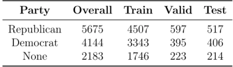
There are 3, 312 distinct speakers in the LIAR dataset with the top five most common ones being ’barack-obama’, ’donald-trump’, ’hillary-clinton’, ’mitt-romney’, and ’john-mccain’. Each distinct speaker has an average of 3.9 claims in the dataset. The claims also have a fairly even distribution of party affiliation between Democrat and Republican parties throughout the train, validation, and test data set as shown in Figure 3.3.

Label Overall Train Valid Test pants-fire 1049 841 116 92 false 2508 1996 263 249 barely-true 2106 1657 237 212 half-true 2632 2119 248 265 mostly-true 2458 1966 251 241 true 2059 1682 69 208

Table 3.2: Label frequency distribution for the LIAR dataset.

There is also credit history metadata for each claim. This metadata contains total counts of pants-fire, false, barely-true, half-true, and mostly-true for each speaker. It is important to note that the true label counts are missing; the reason for this is unclear. As mentioned in the original LIAR paper [Wang, 2017], the label corresponding to the claim being examined must be removed from these counts before using the credit metadata. Otherwise, because many speakers have only one or a few total claims, the credit metadata would act as almost a direct mapping to the label of the claim.

Party Overall Train Valid Test Republican 5675 4507 597 517

Democrat 4144 3343 395 406

None 2183 1746 223 214

Table 3.3: Party affiliation frequency distribution for the LIAR dataset.

To illustrate, if the current label is not removed from the credit metadata, then a naive maximum likelihood model using the credit metadata will result in accura-cies of 43.03%, 45.48%, 43.09% for the training data, validation data, and test data respectively. This is a significantly better performance than any baseline model can perform. If the label of the current statement is removed from the credit metadata, the same maximum likelihood model yields 21.87%, 24.61%, 23.67% accuracy for the training, validation, and test datasets. This is much more reasonable. After this mod-ification, the credit metadata can be used without being unrealistically predictive of the label.

Figure 3-1: Model of a generic CNN as presented in [Kim, 2014]. The input sentence is first converted into a matrix of word vectors. Then, kernels of filter size 2 and 3 are applied, with multiple filters per filter size. The vectors are then pooled and the results are fully connected to a hidden layer.

3.2

Method

For our experiments, we used the Convolutional Neural Network (CNN) architecture, Bidirectional Long Short Term Memory (Bi-LSTM) architecture, and a stacked bidi-rectional LSTM and CNN architecture (Bi-LSTM+CNN). These are similar to the models that were implemented in the original LIAR paper [Wang, 2017], which we use as baselines for comparison.

3.2.1

CNN Architecture

Originally created to be used for image processing problems, CNNs have found ef-fective application in various NLP applications when applied to word embedding matrices [Kim, 2014]. Generally speaking, CNNs contain at least one convolutional layer which takes the input and convolves it over a kernel.

If we define 𝑛 to be the size of the word vector, the convolution kernels are generally of dimensions 𝑖 by 𝑛, where 𝑖 is a positive integer, which produce outputs representing 𝑖-gram models. For example, if the size of the word vector is 300, and the kernel size is 2 by 300, the convolution will convolve two word vectors at a time and output

information corresponding to every consecutive pair of words. In other words, it captures bigram information. Often, more than one kernel size will be used to capture dependencies amongst different numbers of consecutive words.

After convolving the input, a simple but powerful architecture involves connecting the output of the convolutional layer to a hidden layer which is then connected to an output layer. A diagram of such a model, borrowed from previous work [Kim, 2014], is shown in Figure 3-1.

3.2.2

Bi-LSTM Architecture

An older, but equally effective approach to classifying textual content is to use a Long Short-Term Memory (LSTM) model [Hochreiter and Schmidhuber, 1997]. A LSTM is similar to the Recurrent Neural Network (RNN) in that it leverages information from previous inputs for processing the current input. In general for natural language applications, individual words are passed in one at a time to RNNs and the recurrent structure allows each word to utilize information about the previous words. However, RNNs struggle to handle longer sequences of inputs as the information from previous inputs are lost quickly. LSTMs counteract this information loss by using memory units, which can selectively save input information within the cell itself. An example diagram of a LSTM cell can be found in Figure 3-2.

Bidirectional LSTMs are an extension of LSTMs and involve using two LSTMs at once; one which takes sentence input in forward order and the other in backwards order [Graves and Schmidhuber, 2005]. This way, for each input, the model gets sequential information for inputs before and after it. With this extra information, bidirectional LSTMs are able to outperform LSTMs for many tasks [Graves and Schmidhuber, 2005].

3.2.3

Stacked LSTM and CNN Model Architecture

Although the bidirectional LSTM model is capable of remembering information over a long sequence of inputs, it’s not able to capitalize on the n-gram coherence of the

Figure 3-2: Model of a generic LSTM cell as presented by Chen [Chen, 2016]. LSTM cells contain a input and output gates of a LSTM cell control information flow to and from the memory unit. Additionally, LSTM cells have a forget gate, which can be used to remove information from the memory cell.

CNN model. In order to take advantage of the strengths of both models, a stacked bidirectional LSTM and CNN model can be used. The model is created by modifying the previous bidirectional LSTM model to process the input through a bidirectional LSTM layer followed by a CNN layer before being fully connected to a hidden layer. It’s been found that for some applications, using this combination of layers pro-duces better results than using just one. For example, for the problem of question answer matching [Tan et al., 2016], the stacked LSTM and CNN model outperforms both the LSTM only model and the CNN only model. For our work, we will expand on this model by using a bidirectional LSTM rather than just a LSTM as we believe that the extra sequential information will benefit the model. An example of a stacked LSTM and CNN architecture is shown in Figure 3-3.

3.2.4

Evaluation Metrics

Figure 3-3: Diagram of Bi-LSTM and CNN model. The input layer is first fed into the Bi-LSTM layer. The features extracted from the Bi-LSTM layer are then fed into the convolutional layer. Finally, the output from the convolutional layer is fed into a fully connected hidden layer before undergoing classification via a final softmax layer.

(i) Average Accuracy: The accuracy of models averaged over multiple trainings. Accuracy is defined as the number of correctly classified examples divided by their total number of examples.

(ii) Best Accuracy: The accuracy of the trained model with highest validation accuracy. This metric is to allow direct comparison to the results of the original LIAR paper.

3.3

Experiments

For the LIAR task, we optimized baseline models using CNN and bidirectional LSTM architectures in combination with the given metadata. We also experimented with the novel idea of applying the stacked bidirectional LSTM (Bi-LSTM) and CNN model to this task. After tuning some hyperparameters, each of these models exceeds the original LIAR paper significantly in terms of accuracy. Each of the models described

next in this section were implemented using the Keras deep learning library.

3.3.1

CNN Experiments

For our models involving CNNs, we imitated and improved upon the basic construc-tion described in the original LIAR paper [Wang, 2017] with several improvements to improve performance. That construction was inspired by a recently proposed model for using CNNs on text classification problems [Kim, 2014] as discussed in Section 3.2.1.

First, our model converted the input claim into a matrix of word vectors. Although the original paper used Word2Vec [Mikolov et al., 2013a] vectors trained on Google News2_{, we discovered that GloVe [Pennington et al., 2014] vectors performed better}

for the task, particularly the pretrained 840B token common crawl set.3 That matrix of embeddings was then subject to a Keras embedding layer with embedding training enabled. This trained the embeddings to be more specialized for the LIAR dataset, slightly improving the overall performance.

Then, the model convolves the input matrix on filter sizes of 2, 3, and 4 with 128 filters for each filter size. This effectively extracts bigram, trigram and quadgram information about the input claim. Alternative filter amounts and sizes were tried, but no arrangement found improved upon the current setting. A ReLU activation is used for the convolution. After, the convolution output is subject to average pooling. The original construction employed max pooling but we found that average pooling gives much better results. After these operations, a single value is output from each filter.

The model then concatenates all of the output values together into a single vector. That vector is then subject to dropout at a rate of 0.2. If any metadata is used, it is then concatenated to the resulting vector. Finally, the model connects the vector to a fully connected hidden layer with 100 neurons. That layer is then fed into a softmax layer which predicts the claim label. Both the dropout rate and hidden layer

2_{https://github.com/mmihaltz/word2vec-GoogleNews-vectors} 3_{https://nlp.stanford.edu/projects/glove/}

size chosen as a result of tuning.

We trained each model with 20 epochs using the Adam optimizer rather than the traditional Stochastic Gradient Descent which the paper originally used. Using Adam allowed us to use much fewer training epochs and actually allowed training to converge onto better models. The model with lowest validation loss was chosen from training. The model almost always started overfitting to the training data by epoch 5, so fewer training epochs could have been used. The accuracy results for our models and the original reported results can be found in Figure 3.4. Using a TITAN X GPU, each model took less than 5 minutes to train.

3.3.2

Bidirectional LSTM Experiments

For the bidirectional LSTM model (Bi-LSTM), we also converted the input claim into GloVe word vectors and passed the matrix into a Keras embedding layer. The output was then subject to a bidirectional LSTM layer. After tuning, we decided that input and recurrent dropout rates of 0.4 and an output dimension of 64 for the LSTM were approximately optimal. Note that because the LSTM was bidirectional, the actual output dimension was 64 * 2 = 128.

The output vectors after every word was processed through the LSTM were saved and concatenated into one large vector, which was then subject to a dropout at a rate of 0.2. Similar to the CNN model, any metadata was concatenated at this step and the result was fully connected to a 100 neuron hidden layer. That hidden layer is then connected to a softmax layer which predicts the label of the input claim. As before, this model was trained with 20 epochs using the Adam optimizer. Using a TITAN X GPU, each model took less than 15 minutes to train.

3.3.3

Stacked Bidirectional LSTM and CNN Experiments

The Stacked Bidirectional LSTM and CNN model (Bi-LSTM+CNN) takes the matrix of word embeddings from the Keras embedding layer and first processes it through a Bidirectional LSTM layer. After tuning, the same set of parameters for the

Bidirec-tional LSTM also had good results for the combined model; the dropout rates were set to 0.4 and the output dimension was set to 64 for one direction of the LSTM.

Then, the output of the LSTM was passed into the convolutional layer. Again, it turns out that the same parameters for the convolutional layer as the CNN model produced strong results. To reiterate, the filter sizes chosen were 2, 3, and 4 and each filter size had 128 filters. The dropout rate was 0.2 in the convolutional step and average pooling was used. The output of the convolutional layer along with any metadata is then passed through a dropout layer of rate 0.2 and then fully connected to a hidden layer of size 100. Finally, the hidden layer is connected to the softmax layer which predicts the labels. The model was trained with 20 epochs with the Adam optimizer. Using a TITAN X GPU, each model took less than 15 minutes to train.

3.4

Analysis

The results of our experiments are shown in Table 3.4. Our CNN model with any subset of metadata outperformed the original reported results by 1% to 5% across the board in terms of validation accuracy. This lead to a higher test accuracies in general. Furthermore, these results are in line with those reported before, indicating that the model produces consistent results. Next, for the Bi-LSTM model, our models outperformed the previously reported accuracies by more than 5% each. Our results show that the Bi-LSTM model is actually comparable to the CNN models, despite the results that the original paper indicating otherwise. Finally, our stacked Bi-LSTM and CNN model generally performed similarly to the CNN model. This makes sense since the CNN layer was the last layer before the multilayer perceptron used for label prediction. It indicates that the LSTM layer prior to that CNN layer did not provide any additional useful information.

Model Best Val Best Test Avg Val Avg Test

1. Wang-CNN 26.0 27.0 N/A N/A

2. Wang-CNN+subject 26.3 23.5 N/A N/A

3. Wang-CNN+party 25.9 24.8 N/A N/A

4. Wang-CNN+credit 24.6 24.1 N/A N/A

5. Wang-CNN+all 24.7 27.4 N/A N/A

6. Wang-Bi-LSTM 22.3 23.3 N/A N/A

7. CNN 28.0 27.4 27.0 26.3 8. CNN+subject 27.8 26.9 26.3 26.8 9. CNN+party 30.4 27.9 28.3 27.0 10. CNN+credit 29.0 27.5 27.4 27.8 11. CNN+all 30.0 28.6 28.8 28.2 12. Bi-LSTM 27.5 24.6 26.4 25.8 13. Bi-LSTM+subject 27.3 26.8 26.1 25.8 14. Bi-LSTM+party 28.8 26.8 26.6 26.2 15. Bi-LSTM+credit 27.2 25.8 26.0 26.7 16. Bi-LSTM+all 28.3 26.0 26.8 26.3 17. Bi-LSTM+CNN 28.0 28.0 27.0 26.8 18. Bi-LSTM+CNN+subject 27.7 27.0 26.8 27.2 19. Bi-LSTM+CNN+party 29.9 26.3 28.5 26.6 20. Bi-LSTM+CNN+credit 28.8 28.4 27.7 27.6 21. Bi-LSTM+CNN+all 31.0 27.6 28.9 28.1

Table 3.4: Model Accuracy Results. The ’Wang’ prefix denotes results from original LIAR paper [Wang, 2017]. Suffixes subject, party, credit, and all indicate that the corresponding pieces of metadata were used. Best model was picked by choosing the highest validation accuracy model out of 10 trained. Avg indicates average accuracy over 10 trained models.

3.5

Discussion

In addition to the provided metadata, we also experimented with using other meta-data such as part of speech frequency. However, we did not see any significant im-provements with this metadata; in fact performance decreased when it was used. We also tried other model constructions, such as a parallel rather than a stacked Bi-LSTM and CNN model and a stacked CNN Bi-LSTM model in which the CNN layer came first. Both of these models did not improve the performance.

effective way for this task, we believe that even a fully optimized model using these techniques will not significantly exceed the results we presented here. Part of the problem is that the problem space is simply too large for the amount of data provided by the LIAR dataset. Possible approaches to resolve this issue include using additional data or innovating new models which can better utilize existing information. Another possible approach is to break down the fact checking problem into multiple smaller tasks, each with a smaller problem space following a breakdown mentioned in Section 1.2. Then, existing data might be better leveraged to solve these tasks with smaller problem spaces before being combined to create a fact checking system.

In addition, a particular issue with this data is about lack of clarity on how the data labels are defined; the line between adjacent label classes such as barely-true and half-true are especially unclear even for humans. So, it will also be hard for a machine trained on LIAR data to make this distinction as well. Likely, a disambiguation of the label classes will allow for better performance.

Because we could not overcome these challenges for the LIAR task, we pivoted to focus our work on a smaller subproblem of fact checking known as stance detection. This problem has the advantage of having a much small problem space as well as a larger set of available data. We will discuss our experiments regarding stance detection in the next chapter.

3.6

Summary

We presented CNN and bidirectional LSTM (Bi-LSTM) based models for the LIAR dataset which significantly exceeded previous baselines. These results show that both neural models have similar potential in the task, contrary to what previous results showed. Also, we presented other model ideas we tried, such as the stacked CNN and Bi-LSTM model, though these more complex models did not see any significant performance gain.

Chapter 4

Stance Detection using Adversarial

Domain Adaptation

In this chapter, we discuss our work on the stance detection problem. As discussed earlier in Section 1.2, this problem involves automatically determining the perspective of a document relative to a claim. Here, we focus our experiments on the novel idea of applying adversarial domain adaptation to address this problem, particularly when the labeled data is limited.1 _{The upcoming sections will discuss our datasets}

(Sec-tion 4.1), method (Sec(Sec-tion 4.2), experiments (Sec(Sec-tion 4.3) and findings (Sec(Sec-tion 4.4).

4.1

Datasets

For the stance detection problem, we primarily focus on using the Fake News Chal-lenge (FNC) dataset [Pomerleau and Rao, 2017], a publicly available stance detection dataset, to evaluate our models. Since the dataset has very limited labeled data for some label classes, we supplement it with data from the Fact Extraction and VER-ification (FEVER) [Thorne et al., 2018] dataset, an independent stance detection dataset (see Section 4.1.2), and with data from the Stanford Natural Language In-ference (SNLI) [Bowman et al., 2015] dataset, which was created for a related task

1_{Results from a portion of these experiments were published in the 2018 NIPS Continual Learning}

Label Claim Document agree Hundreds of Palestinians

flee floods in Gaza as Israel opens dams

Hundreds of Palestinians were evacu-ated from their homes Sunday morning after Israeli authorities opened a num-ber of dams near the border . . .

disagree Spider burrowed through tourist’s stomach and up into his chest

Fear not arachnophobes, the story of Bunbury’s “spiderman” might not be all it seemed. Perth scientists have cast doubt over claims that a spider bur-rowed into a man’s body during his first trip to Bali . . .

discuss Soon Marijuana May Lead to Ticket, Not Arrest, in New York

Law-enforcement officials tell the New York Times that soon the NYPD may issue tickets for low-level marijuana possession rather than making arrests . . .

unrelated N. Korea’s Kim has leg in-jury but in control

You want a gold Apple Watch, you say? Then it’s going to cost you... a lot. The vanilla variant of Apple’s newest wrist-worn wearable device only costs $349 . . .

Table 4.1: Randomly chosen examples of claim-document pairs and their labels from the FNC dataset. The relevant snippet from each document is displayed.

(i.e., textual inference problem; see Section 4.1.3). Next, we will discuss each of these datasets in depth.

4.1.1

Fake News Challenge

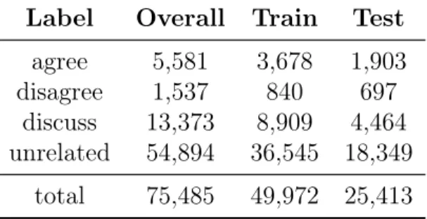
The FNC dataset contains claim-document pairs, with labels which explain the stance relationship between them. The possible labels are agree, disagree, discuss, and unre-lated. Randomly selected samples from the FNC dataset are displayed in Table 4.1. The dataset is partitioned into train and test sets. Combined, there are about 75k claims in total, and the train set has approximately twice as many claims as the test set. Each claim is on average about 11 words long, and each corresponding document is about 360 words long. As shown in Table 4.2, there is a significant imbalance of the frequency of each label class. In particular, the agree and disagree classes have

Label Overall Train Test agree 5,581 3,678 1,903 disagree 1,537 840 697 discuss 13,373 8,909 4,464 unrelated 54,894 36,545 18,349 total 75,485 49,972 25,413

Table 4.2: Label frequency distribution for the FNC dataset.

relatively few data points. Comparing the train and test sets, the label distributions are approximately the same. However, there is a slightly higher proportion of disagree labels in the test set.

4.1.2

Fact Extraction and VERification

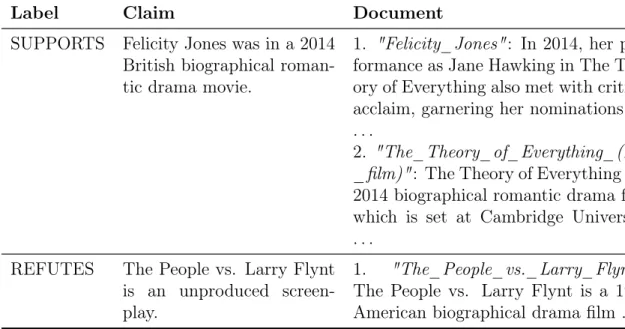
The Fact Extraction and VERification (FEVER) dataset is constructed such that a claim is associated with some number of related Wikipedia documents, each document is assigned as either SUPPORTS or REFUTES label based on its stance relationship to the claim. The claim is then assigned an overall label, either SUPPORTS or RE-FUTES based on its relationship to all of the associated evidence documents. If there are no associated documents, the claim is labeled as NOT ENOUGH INFO. Some randomly chosen examples from the FEVER dataset are displayed in Table 4.3. As shown in Table 4.4, there are about 80k SUPPORTS claims, 30k REFUTES claims, and 35k NOT ENOUGH INFO claims. Since there are no associated documents with NOT ENOUGH INFO claims, we end up not using these labels.

In our work, we use the FEVER dataset to supplement the FNC dataset using the domain adaptation technique by hypothesizing that FEVER SUPPORTS and REFUTES labels are similar to FNC agree and disagree labels respectively. However, we have to reformat the FEVER dataset slightly to make it similar to the format of the FNC dataset in which each example consists of a single document and a single claim. Thus, we break up any claim that is associated with more than a single document into multiple claim-document pairs. For example, the claim shown in the

Label Claim Document SUPPORTS Felicity Jones was in a 2014

British biographical roman-tic drama movie.

1. "Felicity_Jones": In 2014, her per-formance as Jane Hawking in The The-ory of Everything also met with critical acclaim, garnering her nominations for . . .

2. "The_Theory_of_Everything_(2014 _film)": The Theory of Everything is a 2014 biographical romantic drama film which is set at Cambridge University . . .

REFUTES The People vs. Larry Flynt is an unproduced screen-play.

1. "The_People_vs._Larry_Flynt": The People vs. Larry Flynt is a 1996 American biographical drama film . . .

Table 4.3: Randomly chosen examples of data from the FEVER dataset. The name of each document associated with the claim is given in italics, followed by the relevant snippet from the document.

Label Train Dev Test

SUPPORTS 80,035 3,333 3,333 REFUTES 29,775 3,333 3,333 NOT ENOUGH INFO 35,639 3,333 3,333 total 145,449 9,999 9,999

Table 4.4: Label frequency distribution for the FEVER dataset.

first row of Table 4.3 is associated with two documents, and is converted into two separate claim-document pairs. After this modification, we end up with more data points than officially reported by FEVER [Thorne et al., 2018] with around 102k SUPPORTS labels and around 37k REFUTES labels from the train dataset.2 _The

FEVER average claim and document lengths are respectively 8 and 313 words which is almost the same as FNC as explained in Section 4.1.1.

Note that, the FEVER dataset also contains some annotations at the sentence level for each document with respect to its corresponding claim. However, we use the

2_{As the FEVER development and test datasets had not been released at the time of these}

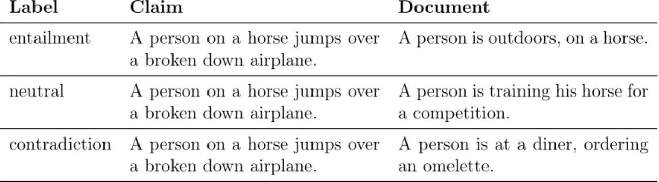
Label Claim Document entailment A person on a horse jumps over

a broken down airplane.

A person is outdoors, on a horse.

neutral A person on a horse jumps over a broken down airplane.

A person is training his horse for a competition.

contradiction A person on a horse jumps over a broken down airplane.

A person is at a diner, ordering an omelette.

Table 4.5: Randomly chosen examples of data from the SNLI dataset. The premise-hypothesis pairs are considered as the claim-document pairs.

Label Train Dev Test entailment 183,416 3,329 3,368 contradiction 183,187 3,278 3,237 neutral 182,764 3,237 3,219 total 549,367 9,844 9,824

Table 4.6: Label frequency distribution for the SNLI dataset.

entire document when we supplement the FNC dataset as the documents in FNC are long length. In contrast, we use the FEVER annotations at the sentence level with the SNLI dataset as the SNLI data consists of sentences (see Section 4.4).

4.1.3

Stanford Natural Language Inference

The Stanford Natural Language Inference (SNLI) dataset was created for the tex-tual inference problem and is significantly larger than either the FNC or FEVER datasets, with about 550k total data points. This dataset contains sentence-sentence pairs (premise-hypothesis pairs) with labels to show whether the two input sentences warrant an entailment, contradict, or neutral relationship to each other. Some ran-domly chosen examples of the SNLI dataset are displayed in Table 4.5. Also, as shown in Table 4.6, the dataset is well balanced with around 183k of data points for each label.

FNC and FEVER datasets (i.e., stance detection). However, the entailment and contradiction labels in SNLI can be considered as being similar to the agree and disagree labels in the FNC dataset and the SUPPORTS and REFUTES labels in the FEVER dataset. It’s also possible to interpret neutral label in SNLI to be similar to discuss in FNC, although the connection is not as strong. In this chapter, we also investigate the impact of using the SNLI dataset through a domain adaptation technique to supplement the FNC and FEVER datasets.

We consider the premise-hypothesis pairs in SNLI as the claim-document pairs. This means both the claim and the document in SNLI are only a single sentence. This results in a notable difference between the average length of the documents in SNLI, around 14 words, and the documents in the FNC and FEVER datasets, a couple hundred words, making it harder to leverage for domain adaptation. Ideally, though, our models can pick some features that are independent of the length of the documents, so that the SNLI data may be able to help improve these features.

4.2

Method

Previously proposed approaches for stance detection generally contain two compo-nents [Baird et al., 2017, Hanselowski et al., 2017, Riedel et al., 2017]: a feature extraction component followed by a class label prediction component. In this thesis, we present a model for stance detection that augments the traditional models with a third component: a domain adaptation component.

Our domain adaptation component uses adversarial learning [Ganin and Lempit-sky, 2014] to encourage the feature extraction component to select common, rather than domain specific, features when input data is from multiple different domains. This allows the model to better leverage source domain for better prediction on data from target domain.

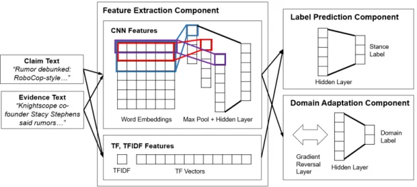
The general architecture of our model is shown in Figure 4-1. As illustrated, the inputs are first given to the “Feature Extraction Component ” to compute their fea-tures and representations. These feafea-tures are then passed to the “Label Prediction

Figure 4-1: The architecture of our model for stance detection which uses adversarial domain adaptation.

Component ” and then to the “Domain Adaptation Component.” In the model, while both latter components try to minimize their own losses, the feature extraction com-ponent attempts to maximize domain classification loss to encourage better mixture of examples from different domains. The components of the model are described in detail below.

4.2.1

Feature Extraction Component

This component takes the input claim 𝑐 and document 𝑑 and converts them to their semantic representations and features. To do this, we use bag of words (BOW) related features, essentially TF and TF-IDF weighted features. We select these BOW features as they are useful to filter documents with unrelated stance labels as we will show in Section 4.4. Furthermore, we also use a convolutional neural network (CNN) approach discussed in Section 3.2.1 for learning representations of claims and documents. To recap, we use a CNN because it can capture 𝑛-grams and long range dependencies [Yu et al., 2014], and can extract discriminative word sequences that are common in the training instances [Severyn and Moschitti, 2015]. These traits make CNNs useful for dealing with long documents [Mohtarami et al., 2016].

4.2.2

Label Prediction Component

The label prediction component uses a multilayer perceptron (MLP) with a fully connected hidden layer followed by a softmax layer which employs cross entropy loss as the cost function. This component will predict stance labels as agree, disagree, discuss, or unrelated for a given set of claim and document features.

4.2.3

Domain Adaptation Component

The domain adaptation component contains a domain classifier which includes a MLP followed by a softmax layer. Given a set of features for a claim-document pair, the domain classifier predicts which domain the features originated from.

The domain classifier acts as an adversary because the model is constructed to encourage the feature extraction component to maximize the domain classifier loss, while the domain adaptation component itself attempts to minimize that same loss. This is because a high domain classifier loss implies that the domain classifier is unable to accurately discern whether a set of features belongs to the source or the target domain. This implies that the features extracted from the input examples are common to both the source and target domains, which is the ultimate goal of the adversarial domain adaptation technique.

To achieve the desired adversarial behavior, the features from the feature extrac-tion component are passed to a gradient reversal layer before being passed to the domain classifier. The gradient reversal layer is a simple identity transform during forward propagation and multiplies the gradient by a negative constant (the gradient reversal constant 𝜆) during backpropagation [Ganin and Lempitsky, 2014]. In partic-ular, if we define the downstream domain loss to be 𝐿𝑑 and the upstream parameters

to be 𝜃𝑓, the gradient reversal layer essentially replaces the partial derivative 𝜕𝐿_𝜕𝜃𝑑

𝑓

with −𝜆𝜕𝐿𝑑

𝜕𝜃𝑓. Effectively, this encourages the upstream components to maximize 𝐿𝑑

while the downstream domain classifier tries to minimize 𝐿𝑑. The desired adversarial

training behavior can be achieved through normal model training.

is generally set to a schedule which starts small and increases steadily during training with:

𝜆𝑝 =

2

1 + 𝑒𝑥𝑝(−𝛾 × 𝑝) − 1 (4.1)

where 𝑝 represents the fraction of training epochs elapsed. This allows the domain classifier to train properly initially before being influenced by the gradient reversal layer. Meanwhile, the learning rate starts high and decays over time with:

𝜇𝑝 =

𝜇0

(1 + 𝛼 × 𝑝)𝛽 (4.2)

where 𝑝 represents the fraction of training epochs elapsed. The learning rate schedule has the dual purpose of encouraging conversion as well as allowing for strong initial domain classifier training. The specific settings for the parameters 𝛾 in domain adap-tation constant, and 𝛼 and 𝜇0 in learning rate formulas are described in Section 4.3.

4.2.4

Model Parameters and Training Procedure

For our CNN model, we use 300-dimensional word embeddings from Word2Vec [Mikolov et al., 2013b], which were trained on Google News, and 100 feature maps with filter width {2, 3, 4}. We set the maximum word lengths of the input claims and documents to be 50 and 500 respectively, where these values are close to the average length for claims and documents in the target train data. For the BOW model, we keep the hyperparameters and features to be the same as the baseline model [Riedel et al., 2017].

Our models are trained using the Adam optimizer, and 20% of the train data is set aside as validation data. In the models with domain adaptation (DA) component, equal amounts of both source and target data are randomly selected at each epoch during training. Finally, we fine tune all the hyperparameters of our models on validation data which contains equal amounts of source and target data.

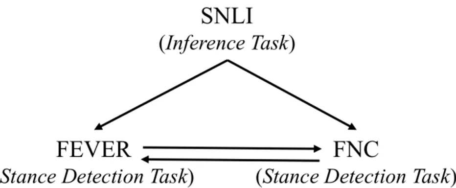
Figure 4-2: Exploring learning with adversarial domain adaptation across different domains (SNLI, FEVER, and FNC datasets) and tasks (stance detection and textual inference tasks).

To reduce domain classifier noise and promote convergence, the gradient reversal constant and learning rate are respectively defined as 𝜆𝑝 and 𝜇𝑝 in Formula 4.1 and

Formula 4.2 in Section 4.2.3. The parameters in the formulas are set to the values that used successfully by previous work [Ganin and Lempitsky, 2014] as 𝛾 = 10, 𝜇0 = 0.01, 𝛼 = 10, 𝛽 = 0.75.

4.3

Experiments

In this chapter, we aim to explore the effect of adversarial domain adaptation across different domains with both similar and dissimilar tasks. As Figure 4-2 shows, the similar tasks are based on stance detection where we consider FNC and FEVER datasets. The dissimilar tasks that we consider are stance detection (FNC or FEVER datasets) and textual inference (SNLI dataset) tasks. We first describe the baselines (Section 4.3.1), evaluation metrics (Section 4.3.2), our models with different config-urations (Section 4.3.3), and then we present our results and analysis across these datasets (Section 4.4).

4.3.1

Baselines

When we use FNC as the target domain, we compare our domain adaptation (DA) model to the following previous work that applied their models on FNC data as target

domain:

(i) Gradient Boosting, which is the Fake News Challenge baseline, and it trains a gradient boosting classifier using handcrafted features reflecting polarity, refute, similarity and overlap between documents and claims.3

(ii) TALOS [Baird et al., 2017], which was ranked first at FNC. It uses a weighted-average between gradient-boosted decision trees (TALOS-Tree) and a deep con-volutional neural network (TALOS-DNN).

(iii) UCL [Riedel et al., 2017], which was ranked third at FNC; this model trains a softmax layer using 𝑛-gram features (e.g., TF and TF-IDF). We compare with this model because our BOW model is similar to it and uses the same features.

Note that, since the FEVER data is a recently released dataset at the time of this work, there has not been any well known baselines available for the dataset. Thus, when we use FEVER data as the target domain, we only perform relative comparisons between our own models.

4.3.2

Evaluation Metrics

We use the following evaluation metrics to evaluate our models: (i) Macro-F1: The average of the 𝐹1 score for each class.

(ii) Accuracy: The number of correctly classified examples divided by their total number of examples.

(iii) Weighted-Accuracy: This metric is presented by Fake News Challenge4 _which

is a two level scoring scheme. It gives 0.25 weight to the correctly predicted examples as related or unrelated. It further gives 0.75 weights to the correctly predicted related examples as agree, disagree, or discuss.

3_{The source code of the FNC baseline is available at https://github.com/FakeNewsChallenge/}

fnc-1-baseline

4

4.3.3

Model Configurations

We present different variations of our models where each uses a subset of components and features shown in Figure 4-1. In particular, we try using different subsets of BOW features and CNN features during feature extraction and try both using and not using the domain adaptation component for each one. These variations help us to conduct ablation analysis on these information sources. The baseline and our models are trained to predict stance labels on target data; {agree, disagree, discuss, unrelated } for target FNC data and {SUPPORTED, REFUTED } for target FEVER data.

For the experiments with target FNC data, we further apply a two level hierarchy prediction scheme in our models, where the first level predicts whether the label is related or unrelated, and then the predicted related labels are passed to the second level to predict agree, disagree, and discuss labels. The reason of using this two level hierarchy scheme with target FNC data is that the current FNC models already perform well for the first level of the hierarchy scheme. For the first level, we use the BOW model which achieves an F1 performance of 97.7% for unrelated and 93.9% for

related labels. Then, the second level is trained with respect to the components and datasets used in the model.

We also conduct specific experiments for certain domain pairs (𝑠𝑜𝑢𝑟𝑐𝑒→𝑡𝑎𝑟𝑔𝑒𝑡): (𝑖) For SNLI→FNC, we map the SNLI neutral labels to the FNC discuss labels to investigate if there is an impact. (𝑖𝑖) For SNLI→FEVER and FNC→FEVER, we balance the label distribution of the data over classes during training and (𝑖𝑖𝑖) we use the annotated sentences of a document that are specified as being relevant to the claim, rather than using the entire document.