HAL Id: hal-00976768
https://hal.inria.fr/hal-00976768v2
Submitted on 27 Dec 2014HAL is a multi-disciplinary open access
archive for the deposit and dissemination of sci-entific research documents, whether they are pub-lished or not. The documents may come from teaching and research institutions in France or
L’archive ouverte pluridisciplinaire HAL, est destinée au dépôt et à la diffusion de documents scientifiques de niveau recherche, publiés ou non, émanant des établissements d’enseignement et de recherche français ou étrangers, des laboratoires
Weak CCP bisimilarity with strong procedures
Luis Pino, Andres Aristizabal, Filippo Bonchi, Frank Valencia
To cite this version:
Luis Pino, Andres Aristizabal, Filippo Bonchi, Frank Valencia. Weak CCP bisimilarity with strong procedures. Science of Computer Programming, Elsevier, 2015, 100, pp.84-104. �10.1016/j.scico.2014.09.007�. �hal-00976768v2�
Weak CCP Bisimilarity with Strong Procedures
✩ Luis F. PinoINRIA/DGA and LIX (UMR 7161 X-CNRS), ´Ecole Polytechnique, 91128 Palaiseau Cedex, France
Andr´es Aristiz´abal
Pontificia Universidad Javeriana Cali
Filippo Bonchi
ENS Lyon, Universit´e de Lyon, LIP (UMR 5668 CNRS ENS Lyon UCBL INRIA), 46 All´ee d’Italie, 69364 Lyon, France
Frank Valencia
CNRS and LIX (UMR 7161 X-CNRS), ´Ecole Polytechnique, 91128 Palaiseau Cedex, France
Abstract
Concurrent constraint programming (CCP) is a well-established model for con-currency that singles out the fundamental aspects of asynchronous systems whose agents (or processes) evolve by posting and querying (partial) information in a global medium. Bisimilarity is a standard behavioral equivalence in concurrency theory. However, only recently a well-behaved notion of bisimilarity for CCP, and a CCP partition refinement algorithm for deciding the strong version of this equivalence have been proposed. Weak bisimilarity is a central behavioral equiv-alence in process calculi and it is obtained from the strong case by taking into account only the actions that are observable in the system. Typically, the standard partition refinement can also be used for deciding weak bisimilarity simply by
us-✩This work has been partially supported by the projects ANR-09-BLAN-0345 CPP, ANR
12IS02001 PACE and ANR-09-BLAN-0169-01 PANDA; and by the French Defense procurement agency (DGA) with a PhD grant.
Email addresses: [email protected](Luis F. Pino), [email protected](Andr´es Aristiz´abal),
[email protected](Filippo Bonchi),
ing Milner’s reduction from weak to strong bisimilarity; a technique referred to as
saturation. In this paper we demonstrate that, because of its involved labeled tran-sitions, the above-mentioned saturation technique does not work for CCP. We give an alternative reduction from weak CCP bisimilarity to the strong one that allows us to use the CCP partition refinement algorithm for deciding this equivalence.
Keywords: Concurrent Constraint Programming, Weak bisimilarity, Partition refinement
1. Introduction
Since the introduction of process calculi, one of the richest sources of foun-dational investigations stemmed from the analysis of behavioral equivalences: in any formal process language, systems which are syntactically different may de-note the same process, i.e., they have the same observable behavior.
A major dichotomy among behavioral equivalences concerns strong and weak equivalences. In strong equivalences, all the transitions performed by a system are deemed observable. In weak equivalences, instead, internal transitions (usually
denoted by τ ) are unobservable. On the one hand, weak equivalences are more
abstract (and thus closer to the intuitive notion of behavior); on the other hand, strong equivalences are usually much easier to be checked (for instance, in [1] a strong equivalence is introduced which is computable for a Turing complete formalism).
Strong bisimilarityis one of the most studied behavioral equivalence and many algorithms (e.g., [2, 3, 4]) have been developed to check whether two systems are equivalent up to strong bisimilarity. Among these, the partition refinement
algo-rithm[5, 6] is one of the best known: first it generates the state space of a labeled transition system (LTS), i.e., the set of states reachable through the transitions; then, it creates a partition equating all states and afterwards, iteratively, refines these partitions by splitting non equivalent states. At the end, the resulting parti-tion equates all and only bisimilar states.
Weak bisimilaritycan be computed by reducing it to strong bisimilarity. Given
a (strong) LTS−→ labeled with actions a, b, τ, . . . one can build a (weak) LTS =⇒
using the following inference rules:
P −→ Qa P =⇒ Qa P =⇒ Pτ P =⇒ Pτ 1 a =⇒ Q1 τ =⇒ Q P =⇒ Qa
Since weak bisimilarity on −→ coincides with strong bisimilarity ona =⇒, thena one can check weak bisimilarity with the algorithms for strong bisimilarity on the
new LTS=⇒.a
Concurrent Constraint Programming(CCP) [7] is a formalism that combines the traditional algebraic and operational view of process calculi with a declarative one based on first-order logic. In CCP, processes (agents or programs) interact by adding (or telling) and asking information (namely, constraints) in a medium (the store). Inspired by [8, 9], the authors introduced in [10] both strong and weak bisimilarity for CCP and showed that the weak equivalence is fully abstract with respect to the standard observational equivalence of [11]. Moreover, a variant of the partition refinement algorithm is given in [12] for checking strong bisimilarity on (the finite fragment of) concurrent constraint programming.
In this paper, first we show that the standard method for reducing weak to strong bisimilarity does not work for CCP and then we provide a way out of the impasse. Our solution can be readily explained by observing that the labels in the LTS of a CCP agent are constraints (actually, they are “the minimal constraints” that the store should satisfy in order to make the agent progress). These constraints
form a lattice where the least upper bound (denoted by⊔) intuitively corresponds
to conjunction and the bottom element is the constrainttrue. (As expected,
tran-sitions labeled by true are internal transitions, corresponding to the τ moves in
standard process calculi). Now, rather than closing the transitions just with respect
to true, we need to close them w.r.t. all the constraints. Formally we build the
new LTS with the following rules.
P −→ Qa
P =⇒ Qa P =⇒ Ptrue
P =⇒ Qa =⇒ Rb
P =⇒ Ra⊔b
The above construction can also be done for CCS [13] by taking sequences
of actions a; b rather than a ⊔ b. Nevertheless, the resulting transition system
may be infinite-branching and hence not amenable to automatic verification using standard algorithms such as partition refinement. In the case of CCP instead, since
⊔ is idempotent, if the original LTS−→ has finitely many transitions, then alsoa
a
=⇒ is finite. This allows us to use the algorithm in [12] to check weak bisimilarity on (the finite fragment) of concurrent constraint programming.
We have developed a tool in which this procedure is implemented. To the best of our knowledge, it is the first tool for checking weak bisimilarity for CCP. It can be found at: http://www.lix.polytechnique.fr/˜andresaristi/ checkers/
Contributions. This paper is an extended version of [14]. In this version we give all the details and proofs omitted in [14]. We generalize some notions, add new examples and extend the intuitions from [14] to improve the clarity of the paper. Furthermore, in Section 3.1.3 we illustrate why our technique would not work for CCS-like process calculi in which two labels cannot be joined into a single one like in CCP. We also add a new section, Section 4, that includes the specification of the algorithm for observational equivalence in CCP, as well as its proof of correctness and complexity. This new section also includes some experiments comparing the strong and weak bisimilarity procedures.
Related Work. CCP is not the only formalism where weak bisimilarity can-not be naively reduced to the strong one. Probably the first case in literature can be found in [2] that introduces an algorithm for checking weak open bisimilarity
ofπ-calculus. This algorithm is rather different from ours, since it is on-the-fly [3]
and thus it checks the equivalence of only two given states (while our algorithm, and more generally all algorithms based on partition refinement, check the equiv-alence of all the states of a given LTS). These algorithms have a polynomial upper bound time complexity. The present algorithm has an exponential time complex-ity. However, they deal with very different formalisms. Also [15] defines weak labeled transitions following the above-mentioned standard method which does not work in the CCP case.
Analogous problems to the one discussed in this paper arise in Petri nets [16, 17], in tile transition systems [18, 19] and, more generally, in the theory of reactive systems [20, 21, 22] (the interested reader is referred to [23] for an overview). In all these cases, labels form a monoid where the neutral element is the label of internal transitions. In the case of CCS, the fact that a system may
perform a transition with a composed labela; b means that it may perform first a
transition witha and then a transition with b. This property, which in tile systems
[18, 19] is known as vertical decomposition, does not hold for CCP and for the other formalisms mentioned above. As a consequence of this fact, when reducing from weak to strong bisimilarity, one needs to close the transitions with respect to the composition of the monoid (and not only with respect to the neutral ele-ment). However, usually, labels composition is not idempotent (as it is for CCP) and thus a finite LTS might be transformed into an infinite one. For this reason, this procedure applied to the afore mentioned cases is not effective for automatic verification.
The result presented in this paper, and more generally our research on CCP, has been largely inspired by the theory of reactive systems by Leifer and Milner [24]: in our operational semantics of CCP, labels represent the “minimal” constraints
that the store should satisfy for executing some transitions, while in [24], labels are the “minimal” contexts.
Structure of the paper. In Section 2 we recall the partition refinement method and the standard reduction from weak to strong bisimilarity. We also recall the CCP formalism, its equivalences, and the CCP partition refinement algorithm. We then show why the standard reduction does not work for CCP. In Section 3 we present our reduction and show its correctness. Finally in Section 4 discuss the decision procedure for observational equivalence in CCP.
2. From Weak to Strong Bisimilarity: Saturation Approach
We start this section by recalling the notion of labeled transition system (LTS), partition and the graph induced by an LTS. Then we present the standard parti-tion refinement algorithm for checking strong bisimilarity, and also how to use it to verify weak bisimilarity. Next we introduce concurrent constraint program-ming (CCP) including the partition refinement algorithm for CCP. Finally, we shall show that the standard reduction from weak to strong bisimilarity does not work for CCP.
Labeled Transition System. A labeled transition system (LTS) is a triple(S, L, )
where S is a set of states, L a set of labels and ⊆ S × L × S a transition
relation. We shall use s a r to denote the transition (s, a, r) ∈ . Given a
transition t = (s, a, r) we define the source, the target and the label as follows
src(t) = s, tar (t) = r and lab(t) = a. We assume the reader to be familiar with the standard notion of bisimilarity [13].
Partition. Given a set S, a partition P of S is a set of non-empty blocks, i.e.,
subsets ofS, that are all disjoint and whose union is S. We write {B1} . . . {Bn}
to denote a partition consisting of (non-empty) blocks B1, . . . , Bn. A partition
represents an equivalence relation where equivalent elements belong to the same
block. We writesPr to mean that s and r are equivalent in the partition P.
LTSs and Graphs. Given a LTS(S, L, ), we write LTS for the directed graph
whose vertices are the states inS and edges are the transitions in . Given a set
of initial states IS ⊆ S, we write LTS (IS ) for the subgraph of LTS rechable
from IS . Given a graph G we write V(G) and E(G) for the set of vertices and
s a s′ a s′′
s, s′, s′′ s, s′ s′′ s s′ s′′
P F (P) F (F (P))
Figure 1: An example of the use of F (P) from Equation 1
2.1. Partition Refinement
We recall the partition refinement algorithm [5] for checking bisimilarity over
the states of an LTS(S, L, ).
Given a set of initial states IS ⊆ S, the partition refinement algorithm (see
Algorithm 1) checks bisimilarity on IS as follows. First, it computes IS⋆ , that
is the set of all states that are reachable from IS using . Then it creates the
partition P0 where all the elements of IS⋆ belong to the same block (i.e., they
are all equivalent). After the initialization, it iteratively refines the partitions by
employing the function on partitions F (−), defined as follows: for a partition
P, sF (P)r iff
ifs a s′ then existsr′ s.t. r a r′ ands′Pr′. (1)
See Figure 1 for an example of F (P). Algorithm 1 terminates whenever
two consecutive partitions are equivalent. In such a partition two states (reachable from IS ) belong to the same block iff they are bisimilar (using the standard notion of bisimilarity [13]).
Algorithm 1 pr(IS , ) Initialization
1. IS⋆ is the set of all states reachable from IS using ,
2. P0 := IS⋆ ,
IterationPn+1 := F (Pn) as in Equation 1
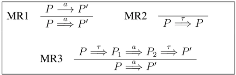
MR1 P a −→ P′ P =⇒ Pa ′ MR2 P =⇒ Pτ MR3 P τ =⇒ P1 a =⇒ P2 τ =⇒ P′ P =⇒ Pa ′
Table 1: Milner’s Saturation Method
Standard reduction from weak to strong bisimilarity. As pointed out in the liter-ature (Chapter 3 in [25]), in order to compute weak bisimilarity, we can use the above-mentioned partition refinement. The idea is to start from the LTS gener-ated using the operational semantics (−→) and then saturate it using the rules
described in Table 1. Now the problem whether two states s and s′ are weakly
bisimilar can be reduced to checking whether they are strongly bisimilar w.r.t.
=⇒. Formally, we can call pr({s, s′}, =⇒) to check whether s and s′are weakly
bisimilar. Henceforth, we shall refer to this as Milner’s saturation method. As we will show later on, this approach does not work in a formalism like CCP. We shall see that the problem is related to the fact that the transitions in CCP are labeled with constraints, thus they can be arbitrary combined (using the least upper bound operator) to form a new label. Notice that this is not the case for the transitions in CCS-like process calculi. Therefore we will need to define a different saturation method to be able to use the saturation approach for verifying weak bisimilarity in CCP. Namely, we will modify the rules in Table 1 so we can still use the standard strategy for deciding observational equivalence in CCP.
2.2. Concurrent Constraint Programming (CCP)
We shall now recall CCP and the adaptation of the partition refinement algo-rithm to compute bisimilarity in CCP [12].
2.2.1. Constraint Systems
The CCP model is parametric in a constraint system (cs) specifying the struc-ture and interdependencies of the information that processes can ask or and add to a central shared store. This information is represented as assertions tradition-ally referred to as constraints. Following [26, 27] we regard a cs as a complete
algebraic lattice in which the ordering⊑ is the reverse of an entailment relation:
element false represents inconsistency, the bottom element true is the empty
con-straint, and the least upper bound (lub)⊔ is the join of information.
Definition 1 (cs). A constraint system (cs) C = (Con, Con0, ⊑, ⊔, true, false)
is a complete algebraic lattice where Con, the set of constraints, is a partially
ordered set wrt ⊑, Con0 is the subset of compact elements of Con,⊔ is the lub
operation defined on all subsets, and true, false are the least and greatest ele-ments of Con, respectively.
Recall that C is a complete lattice if every subset of Con has a least upper
bound in Con. An elementc ∈ Con is finite if for any directed subset D of Con,
c ⊑F D implies c ⊑ d for some d ∈ D. C is algebraic if each element c ∈ Con
is the least upper bound of the finite elements belowc.
In order to model hiding of local variables and parameter passing, in [11] the notion of constraint system is enriched with cylindrification operators and
diagonal elements, concepts borrowed from the theory of cylindric algebras (see [28]).
Let us consider a (denumerable) set of variables Var with typical elements
x, y, z, . . . Define ∃Var as the family of operators∃Var = {∃x | x ∈ Var }
(cylin-dric operators) and DVar as the set DVar = {dxy | x, y ∈ Var } (diagonal
ele-ments).
A cylindric constraint system over a set of variables Var is a constraint system
whose underlying support set Con ⊇ DVar is closed under the cylindric operators
∃Var and quotiented by AxiomsC1 − C4, and whose ordering ⊑ satisfies Axioms
C5 − C7 :
C1. ∃x∃yc = ∃y∃xc C2. dxx = true
C3. if z 6= x, y then dxy = ∃z(dxz ⊔ dzy) C4. ∃x(c ⊔ ∃xd) = ∃xc ⊔ ∃xd
C5. ∃xc ⊑ c C6. if c ⊑ d then ∃xc ⊑ ∃xd
C7. if x 6= y then c ⊑ dxy⊔ ∃x(c ⊔ dxy)
where c, ci, d indicate finite constraints, and ∃xc ⊔ d stands for (∃xc) ⊔ d. For
our purposes, it is enough to think the operator∃xas existential quantifier and the
constraintdxy as the equalityx = y.
Cylindrification and diagonal elements allow us to model the variable
renam-ing of a formulaφ; in fact, by the aforementioned axioms, we have that the
for-mula∃x(dxy⊔ φ) = true can be depicted as the formula φ[y/x], i.e., the formula
obtained fromφ by replacing all free occurrences of x by y.
We assume notions of free variable and of substitution that satisfy the
and fv(c) is the set of free variables of c: (1) if y /∈ fv (c) then (c[y/x])[x/y] = c;
(2)(c⊔d)[y/x] = c[y/x]⊔d[y/x]; (3) x /∈ fv (c[y/x]); (4) fv (c⊔d) = fv (c)∪fv (d).
Example 1 (A Constraint System of Linear Order Arithmetic). Consider the
fol-lowing syntax:
φ, ψ . . . := t = t′ | t > t′| φ ∨ ψ | ¬φ
where the termst, t′can be elements of a set of variables Var , or constant symbols
0, 1, . . .. Assume an underlying first-order structure of linear-order arithmetic
with the obvious interpretation in the natural numbersω of =, > and the constant
symbols.
A variable assignment is a functionµ : Var −→ ω. We use A to denote the
set of all assignments; P(X) to denote the powerset of a set X, ∅ the empty set
and∩ the intersection of sets. We use M(φ) to denote the set of all assignments
thatsatisfy the formulaφ, where the definition of satisfaction is as expected.
We can now introduce a constraint system as follows: the set of constraints
is P(A), and define c ⊑ d iff c ⊇ d. The constraint false is ∅, while true is A.
Given two constraints c and d, c ⊔ d is the intersection c ∩ d. By abusing the
notation, we will often use a formula φ to denote the corresponding constraint,
i.e., the set of all assignments satisfyingφ. E.g. we use x > 1 ⊑ x > 5 to mean M(x > 1) ⊑ M(x > 5). For this constraint system one can show that e is
a compact constraint (i.e., e is in Con0) iff e is a co-finite set in A (i.e., iff the
complement ofe in A is a finite set). For example, x > 10 ∧ y > 42 is a compact
constraint for Var = {x, y}.
From this structure, let us now define the cylindric constraint system S as
follows. We say that an assignmentµ′isanx-variant of µ if ∀y 6= x, µ(y) = µ′(y).
Givenx ∈ Var and c ∈ P(A), the constraint ∃xc is the set of assignments µ such
that existsµ′ ∈ c that is an x-variant of µ. The diagonal element d
xy isx = y.
Remark 1. We shall assume that the constraint system is well-founded and, for
practical reasons, that its ordering⊑ is decidable.
2.2.2. Processes
We now recall the basic CCP process constructions.
Syntax. Let us presuppose a constraint system C= (Con, Con0, ⊑, ⊔, true, false).
The CCP processes are given by the following syntax:
P, Q ::= stop | tell(c) | ask(c) → P | P k Q | P + Q | ∃xP
Finite processes. Intuitively, stop represents termination, the tell process tell(c)
addsc to the global store. This addition is performed regardless of the generation
of inconsistent information. The ask process ask(c) → P may execute P if c is
entailed by the information in the store. The processesP k Q and P + Q stand,
respectively, for the parallel execution and non-deterministic choice ofP and Q;
∃x is a hiding operator, namely it indicates that in∃xP the variable x is local to
P . The occurrences of x in ∃xP are said to be bound. The bound variables of P ,
bv(P ), are those with a bound occurrence in P , and its free variables, fv (P ), are
those with an unbound occurrence1.
Remark 2. In this paper we restrict the CCP syntax to finite processes, since
we shall deal with infinite-state transition system. Typically, to specify infinite behavior, CCP provides parametric process definitions. A processp(~z) is said to
be a procedure call with identifierp and actual parameters ~z. For each procedure
callp(z1. . . zm) there exists a unique (possibly recursive) procedure definition of
the formp(x1. . . xm) def
= P where fv (P ) ⊆ {x1, . . . , xm}. Furthermore recursion
is required to beguarded, i.e., each procedure call withinP must occur within an
ask process. The behavior ofp(z1. . . zm) is that of P [z1. . . zm/x1. . . xm], i.e., P
with eachxireplaced withzi (applyingα-conversion to avoid clashes).
2.2.3. Reduction Semantics
The operational semantics of CCP is given by an unlabeled transition relation
between configurations. A configuration is a pairhP, di representing a state of a
system; d is a constraint representing the global store, and P is a process, i.e., a
term of the syntax. We use Conf with typical elementsγ, γ′, . . . to denote the set
of configurations. A transitionγ −→ γ′ intuitively means that the configurationγ
can reduce toγ′. We call these kind of unlabeled transitions reductions and we use
−→∗to denote the reflexive and transitive closure of−→. Formally, the reduction
semantics of CCP is given by the relation−→ defined in Table 2.
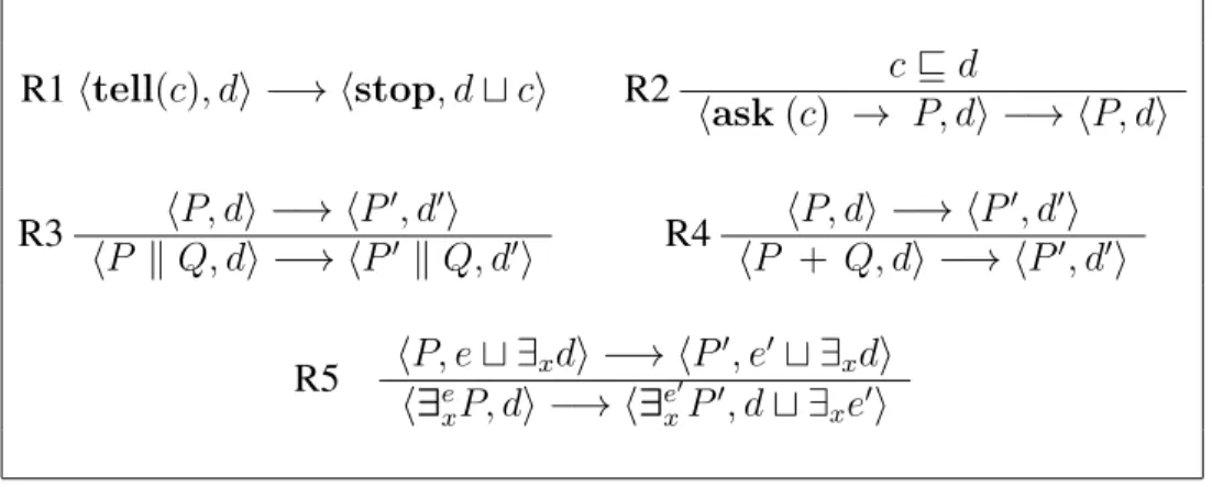
Rules R1, R3 and R4 are easily seen to realize the intuitions described in Section 2.2.2. Rule R2 states that ask(c) → P can evolve to P whenever the
global store d entails c. Rule R5 is somewhat more involved. Intuitively, ∃exP
behaves likeP , except that the variable x possibly present in P must be considered
local, and that the information present in e has to be taken into account. 2 It is
1Notice that we also defined fv(.) on constraints in the previous section. 2Notice that in the syntax we have
∃xP which refers to ∃ e
xP when e = true, namely a local
R1htell(c), di −→ hstop, d ⊔ ci R2 c ⊑ d hask (c) → P, di −→ hP, di R3 hP, di −→ hP ′, d′i hP k Q, di −→ hP′ k Q, d′i R4 hP, di −→ hP′, d′i hP + Q, di −→ hP′, d′i R5 hP, e ⊔ ∃xdi −→ hP ′, e′⊔ ∃ xdi h∃e xP, di −→ h∃e ′ xP′, d ⊔ ∃xe′i
Table 2: Reduction semantics for CCP (symmetric rules for R3 and R4 are omit-ted).
convenient to distinguish between the external and the internal points of view.
From the internal point of view, the variable x, possibly occurring in the global
stored, is hidden. This corresponds to the usual scoping rules: the x in d is global,
hence “covered” by the localx. Therefore, P has no access to the information on
x in d, and this is achieved by filtering d with ∃x. Furthermore, P can use the
information (which may also concern the localx) that has been produced locally
and accumulated ine. In conclusion, if the visible store at the external level is d,
then the store that is visible internally byP is e ⊔ ∃xd. Now, if P is able to make
a step, thus reducing to P′ and transforming the local store intoe′, what we see
from the external point of view is that the process is transformed into∃ex′P′, and
that the information ∃xe present in the global store is transformed into ∃xe′. To
show how this works we show an instructive example.
Example 2. Consider the constraint system from Example 1 and let Var = {x}.
LetP = ∃ex(ask (x > 10) → Q) with local store e = x > 42, and global store
d = x > 2. R2 R5 (x > 10) ⊑ e ⊔ ∃xd = (x > 42 ⊔ ∃x(x > 2)) hask (x > 10) → Q, e ⊔ ∃xdi −→ hQ, e ⊔ ∃xdi hP, di −→ h∃e xQ, d ⊔ ∃xei
Note that the x in d is hidden, by using existential quantification in the
one bound by the local process. Otherwise the ask process ask(x > 10) → Q
would not be executed since the guard is not entailed by the global store d. Rule
R2 applies since(x > 10) ⊑ e ⊔ ∃xd. Note that the free x in e ⊔ ∃xd is hidden in
the global store, i.e. d ⊔ ∃xe, to indicate that is different from the global x.
Remark 3. Observe that any transition is generated either by a process tell(c)
or by a process ask (c) → Q. We say that a process P is active in a transition
t = γ −→ γ′ if it generates such transition; i.e if there exist a derivation of t
where R1 or R2 are used to produce a transition of the formhP, di −→ γ′′.
Barbed Semantics.The authors in [10] introduced a barbed semantics for CCP. Barbed equivalences have been introduced in [29] for CCS, and have become the standard behavioral equivalences for formalisms equipped with unlabeled reduc-tion semantics. Intuitively, barbs are basic observareduc-tions (predicates) on the states
of a system. In the case of CCP, barbs are taken from the underlying set Con0 of
the constraint system.
Definition 2 (Barbs). A configuration γ = hP, di is said to satisfy the barb c
(γ ↓c) iffc ⊑ d. Similarly, γ satisfies a weak barb c (γ ⇓c) iff there exist γ′ s.t.
γ −→∗ γ′ ↓c.
To explain this notion consider the following example.
Example 3. Consider the constraint system from Example 1 and let Var = {x}.
Let γ = hask (x > 10) → tell(x > 42), x > 10i. We have γ ↓x>5 since
(x > 5) ⊑ (x > 10) and γ ⇓x>42 since γ −→ htell(x > 42), x > 10i −→
hstop, (x > 42)i ↓x>42.
In this context, the equivalence proposed is the saturated bisimilarity [8, 9]. Intuitively, in order for two states to be saturated bisimilar, then (i) they should expose the same barbs, (ii) whenever one of them moves then the other should reply and arrive at an equivalent state (i.e. follow the bisimulation game), (iii) they should be equivalent under all the possible contexts of the language. In the case of CCP, it is enough to require that bisimulations are upward closed as in condition (iii) below.
Definition 3 (Saturated Barbed Bisimilarity). A saturated barbed bisimulation
is a symmetric relation R on configurations s.t. whenever (γ1, γ2) ∈ R with
γ1 = hP, ci and γ2 = hQ, di implies that:
(ii) ifγ1 −→ γ1′ then there existsγ2′ s.t.γ2 −→ γ2′ and(γ1′, γ2′) ∈ R,
(iii) for everya ∈ Con0,(hP, c ⊔ ai, hQ, d ⊔ ai) ∈ R.
We say thatγ1 andγ2 are saturated barbed bisimilar (γ1 ∼˙sb γ2) if there exists a
saturated barbed bisimulationR s.t. (γ1, γ2) ∈ R.
We use the term “saturated” to be consistent with the original idea in [8, 9]. However, “saturated” in this context has nothing to do with the Milner’s “satura-tion” for weak bisimilarity. In the following, we will continue to use “saturated” and “saturation” to denote these two different concepts.
Example 4. Consider the constraint system from Example 1 and let Var = {x}.
Take P = ask (x > 5) → stop and Q = ask (x > 7) → stop. One
can check that P 6 ˙∼sb Q since hP, x > 5i −→, while hQ, x > 5i 6−→. Then
considerhP + Q, truei and observe that hP + Q, truei ˙∼sbhP, truei. Indeed, for
all constraints e, s.t. x > 5 ⊑ e, both the configurations evolve into hstop, ei,
while for alle s.t. x > 5 6⊑ e, both configurations cannot proceed. Since x > 5 ⊑ x > 7, the behavior of Q is somehow absorbed by the behavior of P .
As we mentioned before, we are interested in deciding the weak version of the
notion above. Then, weak saturated barbed bisimilarity ( ˙≈sb) is obtained from
Definition 3 by replacing the strong barbs in condition (i) for its weak version (⇓) and the transitions in condition (ii) for the reflexive and transitive closure of the
transition relation (−→∗). Formally,
Definition 4 (Weak Saturated Barbed Bisimilarity). A weak saturated barbed
bisimulation is a symmetric relationR on configurations s.t. whenever (γ1, γ2) ∈
R with γ1 = hP, ci and γ2 = hQ, di implies that:
(i) ifγ1 ⇓ethenγ2 ⇓e,
(ii) ifγ1 −→∗ γ1′ then there existsγ2′ s.t.γ2 −→∗ γ2′ and(γ1′, γ2′) ∈ R,
(iii) for everya ∈ Con0,(hP, c ⊔ ai, hQ, d ⊔ ai) ∈ R.
We say that γ1 and γ2 are weak saturated barbed bisimilar (γ1 ≈˙sb γ2) if there
exists a weak saturated barbed bisimulationR s.t. (γ1, γ2) ∈ R.
LR1htell(c), di −→ hstop, d ⊔ citrue LR2 α ∈ min{a ∈ Con0| c ⊑ d ⊔ a } hask (c) → P, di−→ hP, d ⊔ αiα LR3 hP, di α −→ hP′, d′i hP k Q, di−→ hPα ′ k Q, d′i LR4 hP, di−→ hPα ′, d′i hP + Q, di−→ hPα ′, d′i LR5 hP [z/x], e[z/x] ⊔ di α −→ hP′, e′⊔ d ⊔ αi h∃e xP, di α −→ h∃ex′[x/z]P′[x/z], ∃x(e′[x/z]) ⊔ d ⊔ αi with x 6∈ fv (e′), z 6∈ fv (P ) ∪ fv (e ⊔ d ⊔ α)
Table 3: Labeled semantics for CCP (symmetric rules for LR3 and LR4 are omit-ted).
Example 5. Consider P and Q as in Example 4. We shall prove that P ˙≈sbQ.
First notice that hP, truei 6−→ and also hQ, truei 6−→. Moreover, since none
of the processes has the ability of adding information to the store, then for all
a ∈ Con0,hP, ai ⇓e iffe ⊑ a iff hQ, ai ⇓e. Recall from Example 4 thatP 6 ˙∼sbQ
since an observer can plugP into x > 5 and observe a reduction, which cannot
be observed with Q. Instead P ˙≈sbQ since, intuitively, the discriminating power
of ˙≈sbcannot observe any reductions.
2.2.4. Labeled Semantics
As explained in [10], in a transition of the formhP, di−→ hPα ′, d′i the label α
represents a minimal information (from the environment) that needs to be added
to the store d to evolve from hP, di into hP′, d′i, i.e., hP, d ⊔ αi −→ hP′, d′i.
As a consequence, the transitions labeled with the constraint true are in one to one correspondence with the reductions defined in the previous section. For this
reason, hereafter we will sometimes write −→ to mean −→. Before formallytrue
introducing the labeled semantics, we fix some notation.
Notation 1. We will use to denote a generic transition relation on the state
space Conf and labels Con0. Also in this case mean true
initial configurations IS , we shall use Config (IS ) to denote the set of reachable
configurations3using , i.e.:
Config (IS ) = {γ′ | ∃γ ∈ IS s.t. γ α1 . . . αn γ′for somen ≥ 0}
The LTS(Conf , Con0, −→) is defined by the rules in Table 3. The rule LR2,
for example, says that hask (c) → P, di can evolve to hP, d ⊔ αi if the
en-vironment provides a minimal constraint α that added to the store d entails c,
i.e., α ∈ min{a ∈ Con0| c ⊑ d ⊔ a}. Note that assuming that (Con, ⊑)
is well-founded (Remark 1) is necessary to guarantee that α exists whenever
{a ∈ Con0| c ⊑ d ⊔ a} is not empty. The rule LR5 in Table 3 uses in the
antecedent derivation a fresh variable z that acts as a substitute for the free
oc-currences ofx in P and its local store e. (Recall that T [z/x] represents T with x
replaced withz). This way we identify with z the free occurrences of x in P and e
and avoid clashes with those inα and d. The other rules are easily seen to realize
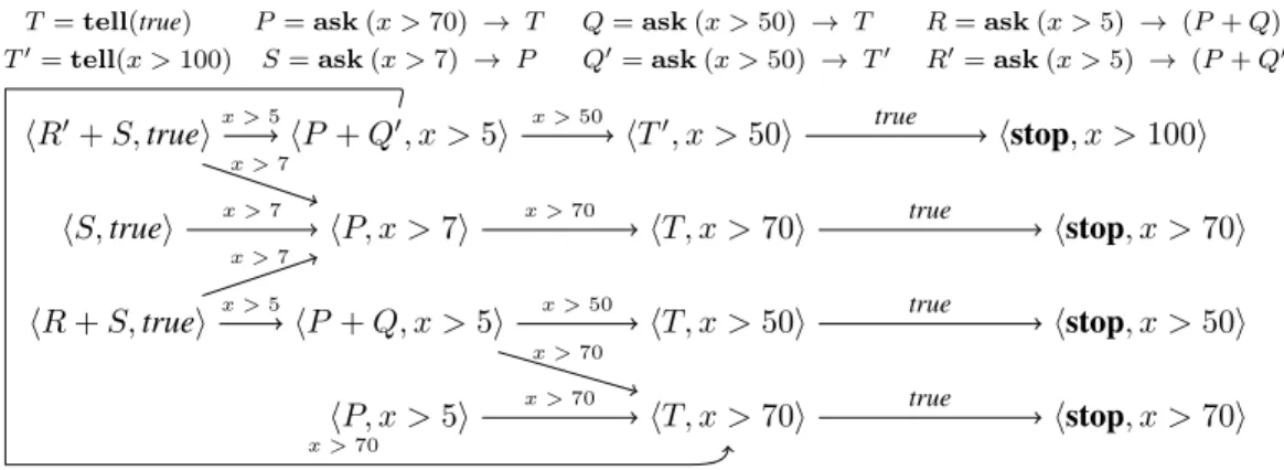
the intuition given in Section 2.2.2. Figure 2 illustrates the LTSs of our running example.
To better understand the labeled semantics consider the following example.
Example 6. Letγ1 = htell(true), truei and γ2 = hask (c) → tell(d), truei.
We can show that γ1 ≈˙sb γ2 when d ⊑ c. Intuitively, this corresponds to the
fact that the implication c ⇒ d is equivalent to true when c entails d. Note
that LTS−→(γ1) and LTS−→(γ2) are the following: γ1 −→ hstop, truei and
γ2 c
−→ htell(d), ci −→ hstop, ci. Consider now the relation R as follows:
R = {(γ2, γ1), (γ2, hstop, truei), (htell(d), ci, hstop, ci), (hstop, ci, hstop, ci)}
One can verify that the symmetric closure ofR is a weak saturated barbed
bisim-ulation as in Definition 3.
The labeled semantics is sound and complete w.r.t. the unlabeled one.
Sound-ness states thathP, di−→ hPα ′, d′i corresponds to our intuition that if α is added
to d, P can reach hP′, d′i. Completeness states that if we add a to (the store in)
hP, di and reduce to hP′, d′i, it exists a minimal information α ⊑ a such that
hP, di−→ hPα ′, d′′i with d′′ ⊑ d′.
The following lemma is an extension of the one in [10] which considers non-deterministic CCP.
3
Notice that when IS⋆
denotes the set of reachable configurations then Config (IS ) = IS⋆
T = tell(true) T′ = tell(x > 100) P = ask (x > 70) → T S = ask (x > 7) → P Q = ask (x > 50) → T Q′ = ask (x > 50) → T′ R = ask (x > 5) → (P + Q) R′ = ask (x > 5) → (P + Q′ ) hR + S, truei hS, truei hR′+ S, truei hP + Q′, x >5i hP, x > 7i hP + Q, x > 5i hP, x > 5i hT′, x >50i hT, x > 70i hT, x > 50i hT, x > 70i hstop, x > 100i hstop, x > 70i hstop, x > 50i hstop, x > 70i x > 70 x > 5 x > 7 x > 7 x > 5 x > 7 x > 50 x > 70 x > 50 x > 70 x > 70 true true true true
Figure 2: LTS−→({hR′+ S, truei, hS, truei, hR + S, truei, hP, x > 5i}).
Lemma 1 (Correctness of−→).
(Soundness) IfhP, ci−→ hPα ′, c′i then hP, c ⊔ αi −→ hP′, c′i.
(Completeness) If hP, c ⊔ ai −→ hP′, c′i then there exist α and b such that
hP, ci−→ hPα ′, c′′i where α ⊔ b = a and c′′⊔ b = c′.
Proof. (Soundness) By induction on (the depth) of the inference of hP, di −→α
hP′, d′i. Here we consider only the additional case for the non-deterministic choice.
• Using Rule LR4 (Table 3), take P = Q + R and P′ = Q′ then we have
hQ, di −→ hQα ′, d′i by a shorter inference. By appeal to induction then
hQ, d ⊔ αi −→ hQ′, d′i. Applying Rule R4 (Table 2) to the previous
reduc-tion we gethQ + R, d ⊔ αi −→ hQ′, d′i.
(Completeness) The proof proceeds by induction on (the depth) of the inference of
hP, d⊔ai −→ hP′, d′i. Again, we consider only the case for the non-deterministic
choice.
• Using Rule R4 (Table 2), take P = Q + R and P′ = Q′ then we have
hQ, d ⊔ ai −→ hQ′, d′i by a shorter inference. Note that the active process
generating the transition could be either an ask or a tell (See Remark 3).
Let suppose that the constraint that has been either asked or told is c. If
it is generated by an ask then d′ = d ⊔ a and c ⊑ d ⊔ a. Note that a ∈
{a′ ∈ C on
0|c ⊑ d ⊔ a′}, and then by Remark 1 there exists α ∈ min({a′ ∈
Con0|c ⊑ d ⊔ a′}) such that α ⊑ a. If it is generated by a tell then d′ =
by induction hypothesis we have that there existα and b such that:
hQ, di−→ hQα ′, d′′i
witha = α⊔b and d′ = d′′⊔b. As said formerly the active process generating
this transition could be either an ask or a tell. If it is generated by an ask
thend′′ = d ⊔ α and if it is generated by a tell then α = true and d′′ = d ⊔ c.
Hence in both cases is safe to assume that d′′ = d ⊔ c. Now by Rule LR4
we have that
hQ + R, di−→ hQα ′, d′′i
sinced′′ = d⊔c we say that a = b and that d′ = d⊔a⊔c = d⊔b⊔c = d′′⊔b.
The above lemma is central for deciding bisimilarity in CCP. In fact, we will show later that, for the weak (saturated) semantics, the completeness direction does not hold. From this we will show that the standard reduction from weak to strong does not work.
2.3. Deciding strong bisimilarity for CCP
In this section we recall how to check∼˙sb with a modified version of partition
refinement introduced in [12]. Henceforth, we shall refer to this algorithm as CCP
partition refinement.
2.3.1. Equivalences: Saturated Barbed, Irredundant and Symbolic Bisimilarity
The main problem with checking∼˙sb is the quantification over all contexts.
This problem is addressed in [12] following the abstract approach in [30]. More
precisely, we use an equivalent notion, namely irredundant bisimilarity∼˙I, which
can be verified with CCP partition refinement. As its name suggests,∼˙I only takes
into account those transitions deemed irredundant. However, technically
speak-ing, going from ∼˙sb to ∼˙I requires one intermediate notion, so-called symbolic
bisimilarity. These three notions are shown to be equivalent,∼˙sb = ˙∼sym = ˙∼I.
In the following we recall all of them.
Let us first give some auxiliary definitions. Unlike for the standard partition refinement, we need to consider a particular kind of transitions, so-called
irredun-dant transitions. These are those transitions that are not dominated by others, in a given partition, in the sense defined below.
Definition 5 (Transition Derivation). Let t and t′ be two transitions of the form
t = (γ, α, hP′, c′i) and t′ = (γ, β, hP′, c′′i). We say that t derives t′, written
t ⊢D t′, iffα ⊑ β and c′′ = c′⊔ β.
The intuition is that the transitiont dominates t′ iff t requires less (or equal)
information from the environment thant′ does (henceα ⊑ β), and they end up in
configurations which differ only by the additional information inβ not present in
α (hence c′′= c′⊔ β). To better explain this notion let us give an example.
Example 7. Consider the following process:
P = (ask (x > 10) → tell(x > 42)) + (ask (x > 15) → tell(x > 42))
and letγ = hP, truei. Now let t1andt2 be transitions defined as:
t1 = γ
x>10
−→ htell(x > 42), x > 10i and t2 = γ
x>15
−→ htell(x > 42), x > 15i
One can check that t1 ⊢D t2 since (x > 10) ⊑ (x > 15) and also (x > 15) =
((x > 15) ⊔ (x > 10)).
Notice that in the definition above t and t′ end up in configurations whose
processes are syntactically identical (i.e.,P′). The following notion parameterizes
the notion of dominance w.r.t. a relation on configurationsR (rather than fixing it
to the identity on configurations).
Definition 6 (Transition Derivation w.r.t. R). We say that the transition t derives
a transitiont′ w.r.t a relation on configurationsR, written t ⊢
R t′, iff there exists
t′′such thatt ⊢
D t′′, lab(t′′) = lab(t′) and tar (t′′)R tar (t′).4
To better understand this definition consider the following example. Example 8. Consider the following processes:
Q1 = (ask (b) → (ask (c) → tell(d))) and Q2 = (ask (a) → stop)
Now let P = Q1 + Q2 where d ⊑ c and a ⊏ b. Then take γ = hP, truei and
consider the transitionst and t′ as:
t = γ −→ hstop, ai and ta ′ = γ −→ hask (c) → tell(d), bib
4Recall that for a given transition t= (s, a, r) the source, the target and the label are src(t) =
Finally, let R = ˙≈sb and take t′′ = (γ, b, hstop, bi) which is constructed
us-ing the target process in t and the label in t′. One can check that t ⊢ R t′
as in Definition 8. Firstly, t ⊢D t′′ follows from a ⊏ b. Secondly, we know
tar(t′′)R tar (t′) from Example 6, i.e. hstop, bi ˙≈
sbhask (c) → tell(d), bi since
hstop, truei ˙≈sbhask (c) → tell(d), truei.
Now we introduce the concept of domination, which consists in strengthening the notion of derivation by requiring labels to be different.
Definition 7 (Transition Domination). Let t and t′ be two transitions of the form
t = (γ, α, hP′, c′i) and t′ = (γ, β, hP′, c′′i). We say that t dominates t′, written
t ≻D t′, ifft ⊢D t′andα 6= β.
As we did for derivation, we now parameterize the notion of domination as follows.
Definition 8 (Transition Domination w.r.t. R and Irredundant Transition w.r.t. R).
We say that the transition t dominates a transition t′ w.r.t a relation on
configu-rationsR, written t ≻R t′, iff there existst′′ such thatt ≻D t′′, lab(t′′) = lab(t′)
and tar(t′′)R tar (t′). A transition is said to be redundant w.r.t. to R when it is
dominated by another w.r.t. R, otherwise it is said to be irredundant w.r.t. to R. We are now able to introduce symbolic bisimilarity. Intuitively, two
configu-rations γ1 and γ2 are symbolic bisimilar iff (i) they have the same barbs and (ii)
whenever there is a transition fromγ1
α
−→ γ′
1, then we require thatγ2 must reply
with a similar transitionγ2
α
−→ γ′
2 (whereγ1′ andγ2′ are now equivalent) or some
other transition that derives it. In other words, the move from the defender does not need to use exactly the same label, but a transition that is “stronger” (in terms
of derivation⊢D) could also do the job. Formally we have the definition below.
Definition 9 (Symbolic Bisimilarity). A symbolic bisimulation is a symmetric
re-lation R on configurations s.t. whenever (γ1, γ2) ∈ R with γ1 = hP, ci and
γ2 = hQ, di implies that:
(i) ifγ1 ↓ethenγ2 ↓e,
(ii) ifhP, ci −→ hPα ′, c′i then there exists a transition t = hQ, di −→ hQβ ′, d′′i
and a stored′s.t. t ⊢
D hQ, di
α
hQ′, d′i and hP′, c′iRhQ′, d′i.
We say thatγ1 andγ2 are symbolic bisimilar (γ1 ∼˙sym γ2) if there exists a
Let us illustrate the definition above by using the process in Figure 2. Example 9. Consider the following processes:
T = tell(true), P = ask (x > 5) → T and Q = ask (x > 7) → T
We provide a symbolic bisimulation
R = {(hP + Q, truei, hP, truei)} ∪ id
to prove hP + Q, truei ˙∼symhP, truei. Take the pair (hP + Q, truei, hP, truei).
The first condition in Definition 9 is trivial. As for the second one, let us take the transitionhP + Q, truei −→ hT, x > 7i. We have to check that hP, truei isx>7
able to reply with a stronger transition. Thus consider the transitionst and t′ as
follows:
t = hP, truei−→ hT, x > 5i and tx>5 ′ = hP, trueix>7hT, x > 7i
Then we can observe that t ⊢D t′ and hT, x > 7iRhT, x > 7i. The remaining
pairs are trivially verified.
And finally, the irredundant version, which follows the standard bisimulation game where labels need to be matched, however only those so-called irredundant transitions must be considered.
Definition 10 (Irredundant Bisimilarity). An irredundant bisimulation is a
sym-metric relationR on configurations s.t. whenever (γ1, γ2) ∈ R implies that:
(i) ifγ1 ↓ethenγ2 ↓e,
(ii) ifγ1 α
−→ γ′
1and it is irredundant inR then there exists γ2′ s.t.γ2 α
−→ γ′
2and
(γ′
1, γ2′) ∈ R.
We say that γ1 and γ2 are irredundant bisimilar (γ1 ∼˙I γ2) if there exists an
irredundant bisimulationR s.t. (γ1, γ2) ∈ R.
Example 10. LetT , P and Q as in Example 9. We can verify that the relation R in
Example 9 is an irredundant bisimulation to show thathP + Q, truei ˙∼IhP, truei.
We take the pair (hP + Q, truei, hP, truei). The first item in Definition 10 is
obvious. Notice now that hP + Q, truei −→ hT, x > 5i is irredundant (Defi-x>5
hP, truei −→ hT, x > 5i and then hT, x > 5iRhT, x > 5i. The other pairs arex>5
trivially verified. Notice that
hP + Q, truei−→ hT, x > 5i ≻x>5 RhP + Q, truei
x>7
−→ hT, x > 7i
hence hP + Q, truei −→ hT, x > 7i is redundant since (x > 5) ⊏ (x > 7),x>7
therefore it does not need to be matched byhP, truei.
As we said at the beginning, the above-defined equivalences coincide with
saturated barbed bisimilarity (∼˙sb, Definition 3). The proof, given in [12], strongly
relies on Lemma 1.
Theorem 1 ([12]). hP, ci ˙∼IhQ, di iff hP, ci ˙∼symhQ, di iff hP, ci ˙∼sbhQ, di
Using this theorem we can define a modified partition refinement, that consider
only the irredundant transitions, in order to compute∼˙sbas we shall see in the next
section.
2.3.2. Partition Refinement for CCP
In [12] we adapted the standard partition refinement procedure to decide strong
bisimilarity for CCP (∼˙sb). As we did for the standard partition refinement, we
start with Config−→(IS ), that is the set of all states that are reachable from the
set of initial state IS using −→. However, in the case of CCP some other states
must be added to IS⋆ in order to verify∼˙sbas we will explain later on.
First, since configurations satisfying different barbs are surely different, the algorithm can be safely started with a partition that equates each state satisfying
the same barbs. Hence, as initial partition of IS⋆ , we takeP0 = {B
1} . . . {Bm},
whereγ and γ′are inB
i iff they satisfy the same barbs.
We now explain briefly how to compute IS⋆ using the Rules in Table 4. Rules
(ISIS) and (RSIS) say that all the reachable states using the transition relation
from the set of initial states should be included, i.e., Config (IS ) ⊆ IS⋆ .
The rule(RDIS) adds the additional states needed to check redundancy.
Con-sider the transitions t1 = γ
α hP1, c1i and t2 = γ β hP2, c2i with α ⊏ β and c2 = c1 ⊔ β in Rule (RD IS
). Suppose that at some iteration of the
parti-tion refinement algorithm the current partiparti-tion is P and that hP2, c2iPhP1, c2i.
Then, according to Definition 8 the transitionst1 would dominatet2 w.r.tP. This
makes t2 redundant w.r.tP. Since hP1, c2i may allow us to witness a potential
(ISIS) γ ∈ IS γ ∈ IS⋆ (RS IS ) γ ∈ IS ⋆ γ α γ′ γ′∈ IS⋆ (RDIS) γ ∈IS⋆ t1= γ α hP1, c1i t2= γ β hP2, c2i α ⊏ β c2 = c1⊔ β hP1, c2i ∈ IS⋆
Table 4: Rules for generating the states used in the partition refinement for ccp
partitionP0, also in the block ofP0wherehP
2, c2i is). See [12] for further details
about the computation of IS⋆ .
Finally, instead of using the function F (P) of Algorithm 1, the partitions are
refined by employing the function IR (P) defined as follows:
Definition 11. (Refinement function for CCP) Given a partition P we define
IR (P) as follows: γ1IR (P) γ2iff
ifγ1 α
γ1′ is irredundant w.r.t. P then there exists γ′ 2 s.t.γ2
α
γ2′ andγ1′ Pγ′ 2
Using this function, the partition refinement algorithm for CCP is defined as follows:
Algorithm 2 pr-ccp(IS , ) Initialization
1. Compute IS⋆ with the rules(ISIS), (RSIS), (RDIS) defined in Table 4,
2. P0 = {B
1} . . . {Bm} is a partition of IS⋆ whereγ and γ′ are inBiiff they
satisfy the same barbs (↓c),
IterationPn+1 := IR (Pn) as in Definition 11
Termination IfPn = Pn+1then returnPn.
Algorithm 2 can be used to decide∼˙sb with exponential time whenever the set
of reachable states is finite. (Recall that Config−→(IS ) represents the set of states
Theorem 2. ([12]) Let γ and γ′ be two CCP configurations. Let IS = {γ, γ′}
and letP be the output of pr-ccp(IS , −→) in Algorithm 2. If Config−→(IS ) is
finite then:
• γ P γ′ iffγ ˙∼
sbγ′.
• pr-ccp(IS , −→) may take exponential time in the size of Config−→(IS ).
The exponential time is due to construction of the set IS⋆−→ (Algorithm 2, step 1)
whose size is exponential in|Config−→(IS )|.
2.4. Incompleteness of Milner’s saturation method in CCP
As mentioned at the beginning of this section, the standard approach for de-ciding weak equivalences is to add some transitions to the original processes, so-called saturation, and then check for the strong equivalence. In calculi like CCS, such saturation consists in forgetting about the internal actions that make part of a sequence containing one observable action (Table 5). However, for CCP this method does not work. The problem is that the transition relation proposed by Milner is not complete for CCP, hence the relation among the saturated, sym-bolic and irredundant equivalences is broken. In the next section we will provide a stronger saturation, which is complete, and allows us to use the CCP partition
refinement to compute ˙≈sb.
Let us show why Milner’s approach does not work. First, we need to introduce formally the concept of completeness for a given transition relation.
Definition 12 (Completeness). We say that is complete if and only if whenever
hP, c ⊔ ai hP′, c′i then there exist α, b ∈ Con
0 s.t. hP, ci
α
hP′, c′′i where
α ⊔ b = a and c′′⊔ b = c′.
Notice that −→ (i.e the reduction semantics, see Table 2) is complete, and
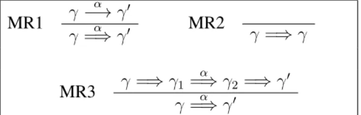
it corresponds to the second item of Lemma 1. Now Milner’s method defines a
MR1 γ α −→ γ′ γ =⇒ γα ′ MR2 γ =⇒ γ MR3 γ =⇒ γ1 α =⇒ γ2 =⇒ γ′ γ =⇒ γα ′
hask α → (ask β → stop), α ⊔ βi
hask β → stop, α ⊔ βi
hstop, α ⊔ βi
hask α → (ask β → stop), truei
hask β → stop, αi
hstop, α ⊔ βi
α
β missing
α ⊔ β
Figure 3: Counterexample for completeness using Milner’s saturation method (cy-cles from MR2 omitted). Both graphs are obtained using Table 5.
new transition relation =⇒ using the rules in Table 5, but it turns out not to be
complete.
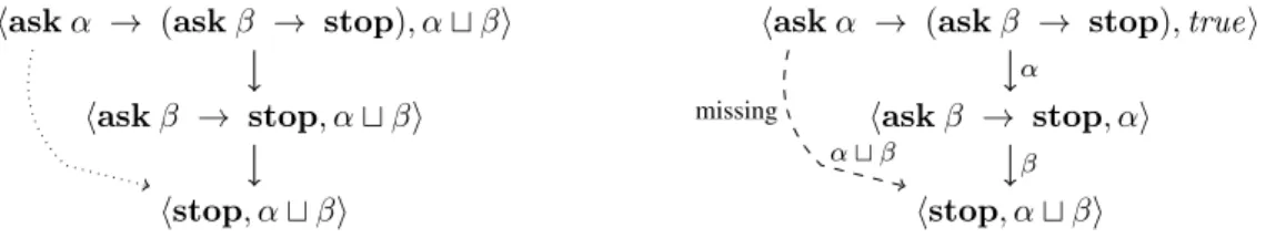
Proposition 1. The relation=⇒ defined in Table 5 is not complete.
Proof. We will show a counter-example where the completeness for=⇒ does not
hold. Let P = ask α → (ask β → stop) and d = α ⊔ β. Now consider the
transitionhP, di =⇒ hstop, di and let us apply the completeness lemma, we can
takec = true and a = α ⊔ β, therefore by completeness there must exist b and
λ s.t. hP, truei =⇒ hstop, cλ ′′i where λ ⊔ b = α ⊔ β and c′′⊔ b = d. However,
notice that the only transition possible is hP, truei =⇒ h(ask β → stop), αi,α
hence completeness does not hold since there is no transition from hP, truei to
hstop, c′′i for some c′′. Figure 3 illustrates the problem.
We can now use this fact to see why the method does not work for computing ˙
≈sb using CCP partition refinement. First, let us redefine some concepts using
the new transition relation =⇒. Because of condition (i) in ˙≈sb, we need a new
definition of barbs, namely weak barbs w.r.t. =⇒.
Definition 13. We sayγ satisfies a weak barb e w.r.t. =⇒, written γ e, if and only
ifγ =⇒∗ γ′ ↓ e.
We shall see later on that coincides with⇓. Using this notion, we introduce
symbolic and irredundant bisimilarity w.r.t. =⇒, denoted by ˙∼=⇒sym and ∼˙=⇒I
re-spectively. They are defined as in Definition 9 and 10 where in condition (i) weak barbs (⇓) are replaced with and in condition (ii) the transition relation is now =⇒. More precisely:
Definition 14 (Symbolic Bisimilarity over =⇒). A symbolic bisimulation over
=⇒ is a symmetric relation R on configurations s.t. whenever (γ1, γ2) ∈ R with
(i) ifγ1 ethenγ2 e,
(ii) ifhP, ci =⇒ hPα ′, c′i then there exists a transition t = hQ, di =⇒ hQβ ′, d′′i
s.t.t ⊢D hQ, di
α
hQ′, d′i and hP′, c′iRhQ′, d′i
We say that γ1 and γ2 are symbolic bisimilar over =⇒, written γ1 ∼˙=⇒sym γ2, if
there exists a symbolic bisimulation over=⇒ s.t. (γ1, γ2) ∈ R.
Definition 15 (Irredundant Bisimilarity over =⇒). An irredundant bisimulation
over=⇒ is a symmetric relation R on configurations s.t. whenever (γ1, γ2) ∈ R:
(i) ifγ1 ethenγ2 e,
(ii) ifγ1 α
=⇒ γ′
1and it is irredundant inR then there exists γ2′ s.t.γ2 α
=⇒ γ′
2and
(γ′
1, γ2′) ∈ R.
We say that γ1 andγ2 are irredundant bisimilar over=⇒, written γ1 ∼˙=⇒I γ2, if
there exists an irredundant bisimulation over=⇒ s.t. (γ1, γ2) ∈ R.
One would expect that since∼˙sb = ˙∼sym = ˙∼I then it is the case that ˙≈sb =
˙
∼=⇒sym = ˙∼=⇒I , given that these new notions are supposed to be the weak versions
of the former ones when using the saturation method. However, completeness is
necessary for proving∼˙sb = ˙∼sym = ˙∼I, and from Proposition 1 we know that
=⇒ is not complete hence we might expect that ˙≈sb does not imply ∼˙=⇒sym nor
˙
∼=⇒
I . In fact, the following counter-example proves this.
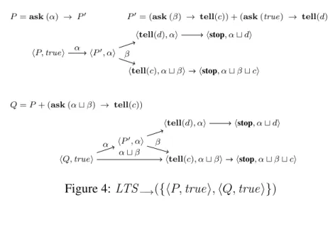
Example 11. LetP, P′andQ as in Figure 4 and 5. Let IS = {hP, truei, hQ, truei}
Figure 4 shows LTS−→(IS ). Figure 5 presents LTS=⇒(IS ) where =⇒ is defined
in Table 5 (Milner’s saturation method).
First, notice thathP, truei ˙≈sb hQ, truei, since there exists a saturated weak
barbed bisimulation:
R = {(hP, truei, hQ, truei)} ∪ id
However, hP, truei 6 ˙∼=⇒
I hQ, truei. To prove that, we need to pick an
irredun-dant transition fromhP, truei or hQ, truei (after saturation) s.t. the other cannot
match. Thus, takehQ, truei−→ htell(c), α ⊔ βi which is irredundant and givenα⊔β
thathP, truei does not have a transition labeled with α ⊔ β then we know that we
cannot find an irredundant bisimulation containing (hP, truei, hQ, truei)
there-fore hP, truei 6 ˙∼=⇒
I hQ, truei. Using the same reasoning we can also show that
˙
P = ask (α) → P′
P′
= (ask (β) → tell(c)) + (ask (true) → tell(d))
hP, truei hP′
, αi
htell(d), αi
htell(c), α ⊔ βi hstop, α ⊔ β ⊔ ci hstop, α ⊔ di α β Q = P + (ask (α ⊔ β) → tell(c)) hQ, truei hP′ , αi htell(d), αi
htell(c), α ⊔ βi hstop, α ⊔ β ⊔ ci hstop, α ⊔ di
α β
α ⊔ β
Figure 4: LTS−→({hP, truei, hQ, truei})
3. Reducing weak bisimilarity to Strong in CCP
In this section we shall provide a method for deciding weak bisimilarity in CCP. As shown in Section 2.4, the usual method for deciding weak bisimilarity (introduced in Section 2.1) does not work for CCP. We shall proceed by redefining =⇒ in such a way that it is sound and complete for CCP. Then we prove that, w.r.t.
=⇒, symbolic and irredundant bisimilarity coincide with ˙≈sb, i.e. ˙≈sb = ˙∼=⇒sym=
˙
∼=⇒
I . We therefore conclude that the partition refinement algorithm in [12] can
be used to verify ˙≈sb w.r.t. =⇒.
3.1. Defining a new saturation method for CCP
If we analyze the counter-example to completeness (see Figure 3), one can see that the problem arises because of the nature of the labels in CCP, namely using
this method hask α → (ask β → stop), truei does not have a transition
withα ⊔ β to hstop, α ⊔ βi, hence that fact can be exploited to break the relation
among the weak equivalences. Following this reasoning, instead of only forgetting about the silent actions we also take into account that labels in CCP can be added together. Thus we have a new rule that creates a new transition for each two consecutive ones, whose label is the lub of the labels in them. This method can also be thought as the reflexive and transitive closure of the labeled transition
relation −→. Such transition relation turns out to be sound and complete and itα
can be used to decide ˙≈sb.
The remaining part of this section is structured as follows. First we define a new saturation method and we proceed to prove that the weak barbs resulting
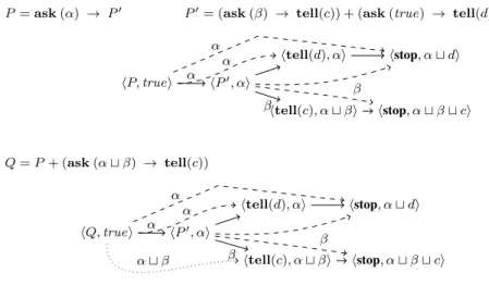
P = ask (α) → P′
P′
= (ask (β) → tell(c)) + (ask (true) → tell(d))
hP, truei hP′
, αi
htell(d), αi
htell(c), α ⊔ βi hstop, α ⊔ β ⊔ ci hstop, α ⊔ di α β α α β Q = P + (ask (α ⊔ β) → tell(c)) hQ, truei hP′ , αi htell(d), αi
htell(c), α ⊔ βi hstop, α ⊔ β ⊔ ci hstop, α ⊔ di α β α ⊔ β α α β
Figure 5: LTS=⇒({hP, truei, hQ, truei}) where =⇒ is defined in Table 5
(Mil-ner’s saturation method). The cycles from rule MR2 are omitted. The dashed transitions are those added by the rules in Table 5. The dotted transition is the
(irredundant) one that hQ, truei can take but hP, truei cannot match, therefore
showing thathP, truei 6˙∼=⇒
I hQ, truei
from such method are consistent with that of CCP (as in Definition 2). Then
under the assumption that −→ is finitely branching we prove that =⇒ is also
finitely branching. Moreover, we follow by showing how this method would be inaccurate in CCS-like formalisms since it could turn a finitely branching LTS into be infinitely branching one. With these elements we can prove soundness and
completeness, which can be finally used to prove the correspondence among ˙≈sb,
˙
∼=⇒
symand∼˙=⇒I .
3.1.1. A new saturation method
Formally, our new transition relation=⇒ is defined by the rules in Table 6.
Remark 4. For simplicity, we shall use the same notation (=⇒) we used for
Milner’s method (Table 5) to denote the new saturation method (Table 6).Con-sequently the definitions of weak barbs, symbolic and irredundant bisimilarity are now interpreted w.r.t. the new=⇒ as in Table 6 ( , ˙∼=⇒symand∼˙=⇒I respectively).
R-Tau γ =⇒ γ R-Label γ−→ γα ′ γ=⇒ γα ′ R-Add γ =⇒ γα ′=⇒ γβ ′′ γ =⇒ γα⊔β ′′
Table 6: New saturation method.
First we show that coincides with⇓ since a transition in =⇒ corresponds to
a sequence of reductions.5
Lemma 2. γ −→∗ γ′iffγ =⇒ γ′.
Proof. (⇒) We can decompose γ −→∗ γ′ as follows γ −→ γ
1 −→ . . . −→
γi −→ γ′, now we proceed by induction oni. The base case is i = 0, then
γ −→ γ′ and by rule R-Label we have γ =⇒ γ′. For the inductive step,
first we have by induction hypothesis thatγ −→i γi impliesγ =⇒ γi (1),
on the other hand, by rule R-Label on γi −→ γ′ we can deduceγi =⇒ γ′
(2). Finally by R-Add on (1) and (2)γ =⇒ γ′.
(⇐) We proceed by induction on the depth of the inference of γ =⇒ γ′. First,
using R-Tau, we can directly concludeγ −→∗ γ. Secondly, using R-Label,
γ =⇒ γ′ implies thatγ −→ γ′. Finally, using R-Add and sinceα ⊔ β =
true implies α = β = true, we get γ =⇒ γ′′ =⇒ γ′ and by induction
hypothesis this means thatγ −→∗ γ′′ −→∗ γ′ thereforeγ −→∗ γ′.
Using this lemma, it is straightforward to see that the notions of weak barbs
coincide.6
Lemma 3. γ ⇓e iffγ e.
Proof. First, let us assume thatγ ⇓e then by definition γ −→∗ γ′ ↓e, and from
Lemma 2 we know thatγ =⇒ γ′ ↓
e, henceγ e. On the other hand, ifγ ethen by
definitionγ =⇒∗ γ′ ↓
e, if we decompose these transitions thenγ =⇒ . . . =⇒ γ′,
and from Lemma 2γ −→∗ . . . −→∗ γ′, thereforeγ −→∗ γ′ ↓
e, finallyγ ⇓e.
As we shall see later on, the lemma above will be used to prove the
correspon-dence between ˙≈sband∼˙=⇒I .
5Notice that Lemma 2 also holds for the Milner’s saturation method (Table 5)
6Notice that Lemma 3 also holds for the Milner’s saturation method (Table 5) because of
3.1.2. The new saturation method is finitely branching
An important property that the labeled transition system defined by the new
relation =⇒ must fulfill is that it must be finitely branching, given that −→ is
also finitely branching. We prove this next but first let us introduce some useful notation.
The set Reach(γ, ), defined below, represents the set of configurations which
results after performing one step starting from a given configurationγ and using
a relation . Such set contains pairs of the form [γ′, α] in which the first item
(γ′) is the configuration reached and the second one (α) is the label used for that
purpose. Formally we have:
Definition 16 (Single-step Reachable Pairs). The set of Single-step reachable
pairs is defined as Reach(γ, ) = {[γ′, α] | γ α γ′}.
We can extend this definition to consider more than one step at a time. We will
call this new set Reach∗(γ, ) and it is defined below.
Definition 17 (Reachable Pairs). The set of reachable pairs is defined as follows:
Reach∗(γ, ) = {[γ′, α] | ∃α 1, . . . , αn. γ α1 . . . αn γ′∧ α = α n}.
Using the notation defined above, we shall define formally what we mean by finitely branching as follows.
Definition 18. We say that a transition relation is finitely branching if for all γ we have |Reach(γ, )| < ∞.
Remark 5. It is worth noticing that even though we have restricted the syntax
of ccp to finite processes, for some constraint systems −→ may be
infinitely-branching due to Rule LR2 in Table 3; i.e., there may be infinitely many mini-mal labels allowing the transition. For this reason we shall sometimes explicitly assume that −→ is defined in constraint systems that do not cause −→ to be
infinitely-branching.
For convenience, in order to project the first or the second item of the
reach-able pairs we will define the functions C and L which, respectively, extract the
configuration and the label respectively (hence the name).
Definition 19. The functionsC and L are defined as follows, C([γ, α]) = {γ} and
L([γ, α]) = {α}. They extend to set of pairs as expected, namely given a set of