en fr

(1)

HAL Id: tel-01897446

https://tel.archives-ouvertes.fr/tel-01897446

Submitted on 17 Oct 2018

HAL is a multi-disciplinary open access

archive for the deposit and dissemination of sci-entific research documents, whether they are pub-lished or not. The documents may come from teaching and research institutions in France or abroad, or from public or private research centers.

L’archive ouverte pluridisciplinaire HAL, est destinée au dépôt et à la diffusion de documents scientifiques de niveau recherche, publiés ou non, émanant des établissements d’enseignement et de recherche français ou étrangers, des laboratoires publics ou privés.

An ordinal generative model of Bayesian inference for

human decision-making in continuous reward

environments

Gabriel Sulem

To cite this version:

Gabriel Sulem. An ordinal generative model of Bayesian inference for human decision-making in continuous reward environments. Cognitive Sciences. Université Pierre et Marie Curie - Paris VI, 2017. English. �NNT : 2017PA066556�. �tel-01897446�

(2)

Université Pierre et Marie Curie

Ecole doctorale Cerveau, Cognition, Comportement

Laboratoire de Neurosciences Cognitives, INSERM U960 / Fonctions du lobe frontal

An ordinal generative model of Bayesian inference for

Human decision-making in continuous reward

environments

Par Gabriel Sulem

Thèse de doctorat de Sciences Cognitives

Dirigée par Etienne Koechlin

Présentée et soutenue publiquement le 14 Septembre 2017

Devant un jury composé de :

Pr. Mathias PESSIGLIONE

Président du Jury

Pr. Peter DAYAN

Rapporteur

Pr. Pierre-Yves OUDEYER

Rapporteur

Dr. Mehdi KHAMASSI

Examinateur

Pr. Etienne KOECHLIN

Directeur de Thèse

(3)

2

Abstract

Our thesis aims at understanding how human behavior adapts to an environment where rewards are continuous. Many works have studied environments with binary rewards (win/lose) and have shown that human behavior could be accounted for by Bayesian inference algorithms. Bayesian inference is very efficient when there are a discrete number of possible environmental states to identify and when the events to be classified (here rewards) are also discrete.

A general Bayesian algorithm works in a continuous environment provided that it is based on a “generative” model of the environment, which is a structural assumption about environmental contingencies which limits the number of possible interpretations of observations and structures the aggregation of data across time. By contrast reinforcement learning algorithms remain efficient with continuous reward scales by efficiently adapting and building value expectations and selecting best options.

The issue we address in this thesis is to characterize which kind of generative model of continuous rewards characterizes human decision-making within a Bayesian inference framework.

One putative hypothesis is to consider that each action attributes rewards as noisy samples of the true action value, typically distributed as a Gaussian distribution. Statistics based on a few samples enable to infer the relevant information (mean and standard deviation) for subsequent choices. We propose instead a general generative model using assumptions about the relationship between the values of the different actions available and the existence of a reliable ordering of action values. This structural assumption enables to simulate mentally counterfactual rewards and to learn

simultaneously reward distributions associated with all actions. This limits the need for exploratory choices and changes in environmental contingencies are detected when obtained rewards depart from learned distributions.

To validate our model, we ran three behavioral experiments on healthy subjects in a setting where reward distributions associated with actions were continuous and changed across time. Our

proposed model described correctly participants’ behavior in all three tasks, while other competitive models, including especially Gaussian models failed.

Our results extend the implementation of Bayesian algorithms to continuous rewards which are frequent in everyday environments. Our proposed model establishes which rewards are “good” and desirable according to the current context. Additionally, it selects actions according to the probability that it is better than the others rather than following actions’ expected values. Lastly, our model answers evolutionary constraints by adapting quickly, while performing correctly in many different settings including the ones in which the assumptions of the generative model are not met.

(7)

6

Introduction

1. Reward

Most of us are familiar with the concept of reward. In many cultural representations of the Wild West, dangerous criminals are wanted, and a reward is offered for their capture. Alternatively, we are supposed to be rewarded for our “good” actions, “good” here either means something positive for society (helping a blind person to cross the street), or qualifies the action as particularly well realized (sales performances). In all these cases a reward is supposed to increase the motivation to perform an action.

It is also a central concept in psychology as a factor in understanding human behavior. It actually has two different origins, which eventually converged (White, 1989). One originates from the writings of Epicurean philosophers which posit that individual behavior is driven by looking for pleasure and avoiding pain. By extension, in a modern psychological view, anything which attracts individuals or animals is a reward; anything which repulses is a punishment or a negative reward (Young, 1959).

The second origin comes from the field of memory creation (today named, learning). The idea of George Ramsay (Ramsay, 1857), later developed experimentally by Thorndike was that a connection between two events (either two stimuli, or a stimuli and an action) is better remembered if it is associated with or followed by a “satisfying state of affairs” (Thorndike, 1911). Because of its effect on the association of the two events, this “satisfying state of affairs” was later named a reinforcer. Rewards are particularly good reinforcers (Skinner, 1938), and these two terms are now used almost equivalently in the literature.

In this chapter we will successively review reward as a drive for behavior, then as a memory reinforcer and describe theories accounting for both.

1.1 Reward as an elementary drive for behavior

For thousands of years people have tried to understand human behavior. Several disciplines, such as philosophy, economics, cognitive sciences, and more, have developed concepts and theories to explain actions and choices.

In psychology, a central concept is reward. Reward is the cause of approach behavior, and is only defined behaviorally. It has been observed and is understood in evolutionary terms as anything that contributes to maintaining homeostasis (for example food), reproduction, or survival (avoiding pain) is rewarding. In a recent review, Wolfram Schultz defines the function of the brain as recognizing and getting rewards in the environment (Schultz, 2015).

Reward is a subjective notion, as different individuals are attracted towards different things, and can vary across time. Rewards also have a magnitude so that prospective rewards can be compared to drive a choice (Samuelson, 1938).

Several approaches have been proposed to measure experimentally the subjective magnitude of reward. For example, the motivation (Berridge, 2004), or effort (Pessiglione et al., 2007) displayed by an animal or human to get something. This variable can be measured in different ways: conscious

(8)

7

reporting, behavioral choices, or physiological measures, and be used as a proxy for reward. Similarly others have tried to measure the “hedonic” pleasure felt during consumption of a good (Plassmann et al., 2008), (Kahneman et al., 1997). Of course nothing guarantees to get the same value scale when different measures are used.

The field of economics is also very interested in human behavior, particularly through

neuro-economics which is a recent subfield aiming at explaining physiological data with economic concepts (Rangel et al., 2008). The central paradigm of economics is the trade-off between cost and gains. Economics postulates the existence of a common scale on which costs and gains can be compared. In particular, all actions have a cost: it can be a physical cost like fatigue, but also an opportunity cost as an action is selected over other potential actions. On the other side, actions have also an expected return in terms of pleasure, survival, money, social prestige, etc. If the return is superior to the cost, the action is performed.

The notion of a personal scale of value on which anything can be compared was first introduced by Bernouilli who spoke of “moral value” (Bernoulli, 1738), and the name “utility” which is still used today in economics was first introduced by Bentham (Bentham, 1781).

Utility is central to explain a choice between several alternatives but there is also no generic way to compute its magnitude. In microeconomics, there are attempts to get a theoretical value. Intuitively, the utility of an umbrella is higher on a rainy day. As a restaurant owner, given some variables (prestige of the restaurant, expected salary, etc.), it could be possible to evaluate the utility of the raw products to buy. But ahead of simple market considerations, these theoretical values are essentially valid to describe the average behavior of a population and there is no real economic model to compute subjective individual “liking” of options. For example, one can generally like red over white wine independent of the relative value of both in the present context (e.g. does it come with meat or cheese?, etc.).

To go further on utility estimation, one can imagine asking people directly to evaluate how much they like or value several items and use their answers as a measure of utility. In behavioral

economics, a common measurement procedure consists of attributing an equivalent monetary value to all things. The “willingness to pay” for a good/service is measured through an auction procedure, which converges to an equivalent value in euros. This value is then used as a proxy for utility (Becker et al., 1964). The prediction is, if the measure is valid, that subsequent choices should follow

predicted utility.

Are reward and utility similar concepts? We discussed above aspects on which reward and utility are similar. A central difference sits in the summation between positive and negative magnitudes. It is experimentally shown that punishments are not equivalent to the inverse of rewards (D’Ardenne et al., 2008). It has been proposed that rewards and punishments are represented on different scales (Fiorillo, 2013), (Frank et al., 2004), and are encoded by different neurotransmitters.

This difference was first pointed out by economists who spotted non-symmetric behavior between losses and gains (Kahneman and Tversky, 1979). However utilities on their side can be added, so that the sum of an equally positive and negative event is theoretically similar to a neutral event.

(9)

8

The framework of utility is very practical to model costs as they can be discounted from the expected utility. However, there is no equivalent operation for physiological rewards. Therefore, even

neurophysiologists are now using the economical concept in their description of biological data: the word “reward” names a positive event which has a “value”. Reward values correspond to subjective utility and can be manipulated as the economic notion. For example Camillo Padoa Schioppa and John Assad claim that the brain encodes the economic value of rewards (Padoa-Schioppa and Assad, 2006).

One of the difficulties of the economic approach is the need to put a value on everything, including friendship, physical integrity, reading a book. If one accepts to have an arm broken for €10 billion, does it mean that this is the actual utility of one’s arm?

To solve this issue, another school of thought in the field of economics has refused to compute cardinal scales to value everything. Instead, they claim that preferences can only be ordered without a notion of absolute distance between the different possibilities. This order can be inferred through choices (Pareto, 1906). Intuitively, if I prefer A to B, then A will be ranked before B. One of the problems is that human or monkey choices can be non-transitive, A can be preferred to B, B to C, but also C to A. In sane humans, the proportion of non-transitive choice is around 3% (Fellows and Farah, 2007). This invalidates the existence of an absolute order in human minds, but it is a sufficiently low proportion, so that absolute order can be used as an approximation.

Economics and psychology explain choices by a comparison of value. Where and how these values are encoded in the brain?

1.1.1 Representation of rewards in the brain

The rewarding dimension of an object is independent of its sensory properties. We have external receptors like eyes and ears to evaluate different sensory properties of objects, but is there something like a reward receptor in charge of encoding reward value?

A large brain network has been identified as the “reward system”. It is defined as brain structures activated when a reward is obtained. The reward system principally includes fronto-basal ganglia loops and thalamo-cortical loops. It has been initially characterized with the technique of

(10)

9

Figure 1: From Schultz 2015

In particular, dopamine neurons of the Substantia Nigra Compacta (SNc) and of the ventral tegmental area (VTA) were found to scale to the magnitude of the anticipated reward prior to a choice(Morris et al., 2006). These neurons project to the striatum in which the “expected” action-value of all possible options was found to be encoded (Samejima et al., 2005). This same result was also showed in rats (Roesch et al., 2009). Therefore the striatum receives value of all possible options, can pick up the most rewarded and trigger action to obtain it. Importantly, the response of dopamine neurons is independent of the modality of the reward, but depends only on its “expected” value (Ljungberg et al., 1992).

In the cortex, the Orbitofrontal Cortex (OFC) which is particularly well connected to the striatum is known to code the brain equivalent of the utility function (Montague and Berns, 2002). Neurons encoding value have been found in animal OFC by intracranial electrophysiology studies, from the early works of the 1980s (Thorpe et al., 1983). The development of a precise methodology to measure subjective value (from animals’ point of view) by Camillo Padoa-Schioppa and John Assad (Padoa-Schioppa and Assad, 2006) enabled to link their activity to utility in the sense that it is independent of its nature, position, or the action necessary to get it (Padoa-Schioppa, 2011). This result was reproduced in other labs (O’Neill and Schultz, 2010).

(11)

10

In humans, functional-MRI studies have confirmed this result in finding correlations between the activity of OFC and its neighbor, the ventromedial prefrontal cortex, and the “value” of a choice. But the difficulty to define “value” objectively led authors to use close but still different definitions of value. Indeed, Kringelbach & colleagues asked participants explicit pleasantness ratings and used them as “values” that they saw coded in the OFC (Kringelbach et al., 2003). Hilke Plassman et al. have used an economic procedure to measure the “willingness to pay” for a good (Plassmann et al., 2007). Jan Peters et al. worked with real money and fitted a model of temporal discounting to use expected value (Peters and Buchel, 2009). In each study, the activity of OFC was correlated with what was defined as value. The study of Maël Lebreton et al. did not use food or money but different categories of objects, and showed that brain activations (in particular in the OFC) reflected choice procedure by consistent and automatic valuation of items (Lebreton et al., 2009).

Values of reward are encoded in the brain but how are they computed? Are they innate or do they depend upon prior experience? Is it possible for an external observer to anticipate the subjective value of a subject?

1.1.2 Construction of reward value

Approach behavior has been characterized in all species as sensibility to reward. Trees grow their roots where there are the most nutrients, or bacteria follow nutrient gradient by chemotaxis to find food sources (Stocker et al., 2008). According to the behavioral definition of rewards, this

corresponds to a sensitivity to rewards.

We mentioned earlier that to favor gene transmission, rewards could have been tuned by evolution towards survival and breeding. This brings the distinction between primary and secondary rewards. Rewards are primary when they directly contribute to help gene reproduction. Following Wolfram Schultz’s recent review, we can put in this category:

-Eating and drinking when needed. This is part of the homeostasis system.

-Behavior associated with reproduction and parental care to transmit genes appropriately.

-Avoidance of “punishments” which could affect survival and future reproduction (Schultz, 2015).

But we have all experienced desire and motivation for things which are not in this list. For humans, primary among them is money. Similarly, it is easy to have animals approaching a-priori neutral objects when these objects have been frequently paired to a primary reward. Frederic Skinner developed a set-up where hungry animals would be put in a chamber (“Skinner Box”) and get food after pressing a lever. A lever is neutral and initially rats are not particularly approaching the lever. But the box is not that big so as they go all around, they eventually press the lever and get food. Skinner observes that these animals will come back to the lever and their pressing frequency will increase as they learn the association between food and the lever. Therefore, animals become motivated to press the lever. This is named operant conditioning or Skinner conditioning (Skinner, 1938). Money or lever pressing are secondary rewards in the sense that it has been learned that they predict the future obtaining of primary rewards.

The same signal can be recorded after similar primary and secondary rewards in the brain (Schultz et al., 1997), even if some areas are specific to the sensory properties of some (primary) rewards (Sescousse et al., 2013).

(12)

11

1.1.3 Reward magnitude

As we explained earlier, approach is the behavioral definition of a reward, and avoidance is the behavioral definition of a punishment (which is different from a negative reward). The rewarding, punishing or neutral status of a stimulus can be very easily determined by observing behavior. However to perform choices, individuals also have a sensitivity to the magnitude of the reward, and are able to choose the greater of two. Importantly, this comparison of magnitude happens when choosing between different quantities of the same good (2 apples are better than 1 apple), but also between goods of different nature (apple or orange?).

It is well known that there is no linear relation between quantities of a good and the magnitude of its reward value. The first introduction of the notion of utility was indeed to introduce a concave

relationship between quantity and utility, so that the marginal utility decreases with quantity. This sensitivity is an individual parameter (Lauriola and Levin, 2001).

There is another way to vary reward magnitude of a good: to change the frequency of its delivery. Pascal defined what an optimal choice in this context is, with the notion of expected value. Expected value multiplies the magnitude of a potential gain with the probability to obtain it. In terms of expected value it is equivalent to obtain €10 for sure and €20 with 50% chances (Huygens, 1657). However, the decreasing marginal utility predicts that people are risk averse and prefer the sure option. This means that the value of the reward associated with the sure option has a higher magnitude.

In economics, the framework of expected values has been extensively discussed. Considering the concavity of the utility function, Von Neumann and Morgenstern have made explicit the axioms that should follow an optimal decision maker computing expected utility instead of expected value (Von Neumann and Morgenstern, 1947). Failure to follow these axioms for example the Allais paradox (Allais, 1953) pushed Kahneman and Tversky to develop their prospect theory where they propose that humans have a distorted perception of probabilities (Kahneman and Tversky, 1979). They suggested a new way to compute the magnitude of stochastic rewards: multiplying these distorted probabilities to the utility of the potential gain.

In lab experiments, monetary rewards are often used on humans as we are used to manipulate them and it is easily possible to separately vary magnitudes and probabilities. The field of neuro-economics pushed for similar approaches on animals by varying the magnitude and probability of food or liquid rewards.

1.1.4 Binary vs. Continuous rewards

In the general case, rewards are evaluated on a continuous scale. For example, in the stock market, gains are unpredictable and can be defined with several decimal numbers (+22.47%). The precision is in all cases bounded by human capacities, either reward receptors, or memory limits. In some environments, rewards can only take a finite number of values. For example at a lottery or tombola the prices are defined in advance and only one of them can be obtained. There are also settings where rewards can only take two values. For example, you can have or miss your train. In this last case, we can say the rewards are binary.

There are interesting simplifications when rewards can be modeled as binary. First, when evaluating a choice the expected value combines the different reward values with the probability of obtaining

(13)

12

them. All this information, two numbers per possible reward, needs to be acquired and memorized. In the case of binary rewards, expected value directly reduced to the probability p of obtaining the reward. This is simpler in terms of memory load, and computational load as no summation across possible rewards is needed.

Also when rewards are discrete or continuous, magnitudes can vary on different orders. And obtaining a high magnitude reward (€1000) may justify the sacrifice of little rewards on the short term (€1). There are therefore trade-offs to operate in order to maximize the total received reward. These trade-offs can be complex as a standard result in economics is that the perception of reward value is not similar for delayed rewards than for immediate rewards (Green and Myerson, 2004). When rewards are binary, only the numbers of rewards need to be maximized without accounting for magnitudes.

Binary rewards also simplify choices in the context of uncertainty as values can only vary on the probability dimension. When magnitudes and probabilities vary independently, it is possible to be presented with a choice where 2 options have the same expected value but not the same

uncertainty: do you prefer €10 for sure or €100 with 10% chances? Individual human participants have different preferences for these choices (Harrison and Rutström, 2008), and the concept of risk-liking or risk-aversion is necessary to explain these differences. In the context of binary rewards, choices can be explained without these additional concepts.

Binary rewards are more than 1 or 0. When there is only one possible reward, whatever its

magnitude, it can be modeled as a binary reward. Interestingly, in this case, the response of neurons is also rescaled to a unique binary response independently of the true magnitude of the reward (Tobler et al., 2005). The problem with continuous rewards is that it is always possible to receive higher than expected magnitudes. For example your idea of what is the best food in the world might evolve across life while more and more restaurants are visited. The discovery of a new maximum reconfigures expectations and the definition of an average meal.

In the following chapters, we will often make a distinction between binary and continuous rewards as the treatment of continuity asks for more computational tools. In the following sections of this first chapter, we expose simple inference free decision making methods which apply as well to the continuous case as to the binary case. In the third chapter, we will mention complex inference algorithms which are, for the majority of them, designed for discrete rewards. Our PhD work is aimed at understanding how these algorithms can be extended to an environment presenting continuous rewards.

1.1.5 Critiques of neuro-economics

To conclude this part on reward and its motivational dimension, we would like to review critiques addressed to the use of economic paradigm to study animal and human behavior.

The field of neuro-economics developed on the postulate that natural animal behavior is a rational decision problem of utility maximization (Pearson et al., 2014). However, real life environments are usually open. It means that, contrary to laboratory tasks where choices are proposed between a limited numbers of well-defined options, the different real-life options are not always explicit. If we consider that resources (money, strength, etc.) are limited, getting something also means not getting other things. The choice is then between buying an object, being able to use it, and maybe not being

(14)

13

able to buy other objects. Or nor buying, not being able to use it, but being able to buy something else. Therefore, the theoretical comparison underlying the act of buying in the utility framework asks to consider an infinite number of possibilities (Köszegi and Rabin, 2007).

Also, experimenters have doubted that utility measures are always relevant to explain behavior. For example, a dissociation was shown in animals between how they “want” something to how they “like” it (Berridge, 1996). In particular, habits (Dickinson, 1985) or rules (Sanfey et al., 2003) can guide action away from (otherwise) preferred outcomes. Therefore, measuring reward values creates a pertinent subjective hierarchy between different goods or services, but which is not enough to explain choices in many common settings.

We will now analyze a completely different use of the reward signal which is not at all present in the concept of utility or in economics. In uncertain environments, rewards act as a reinforcer and drive learning.

1.2 Reward as a learning signal

In this section, we will explain the concept of reinforcement in behavioral psychology. Reinforcement names the effect of rewards on the future repetition of the behavior which enables to obtain them.

The goal of behavior is to maximize reward. When the current environment is well known and predictable, this consists of selecting the “best” action, the one with the highest expected reward. For example, in your favorite bakery you know exactly which bread is the best, and what is your second choice if the first choice is not available. In an unknown environment, what is the best strategy to both learn and maximize reward concomitantly? What is experimentally observed on animals and humans?

Learning experiments on animals have more than a century of history. Thorndike put cats in a puzzle box, and measured how fast they would find the trick to escape, knowing that food is available outside. He noticed that animals would at the beginning find the exit by chance, but once put again in the box, they would reliably be faster to exit until they eventually “learned” to do it immediately. Thorndike suggested that the reward obtained out of the box facilitates the memorization of the correct action (the one which allows getting out) (Thorndike, 1911).

By chance, while he was studying digestion mechanisms in dogs, Pavlov noticed that a neutral stimulus could become so predictive of a reward in animal’s mind, that their reaction to the stimulus would be the same as their reaction to the reward (Pavlov, 1927).

(15)

14

Figure 2: Classical conditioning, whistle sound is associated with food and cause the same response than food. From Beginning Psychology, Charles Stangor 2012

In Figure 2 the whistle sound is initially neutral, while food is a rewarding stimulus which causes salivation. After conditioning, the whistle sound by itself causes salivation. The presentation of reward has reinforced the predictive ability of the food by the sound. This is named Pavlovian or classical conditioning.

We already mentioned the work of Frederick Skinner. Interestingly, in operant or Skinner

conditioning, it is the action which is predictive of the reward and therefore animals are motivated to perform it. In an unknown environment, conditioning predicts that animals will repeat rewarded actions and avoid punished actions.

Is there a mathematical way to model this reward dependent learning? In particular, is it possible to predict the subjective value of an action, knowing the history of reward and punishment that were obtained after it was performed?

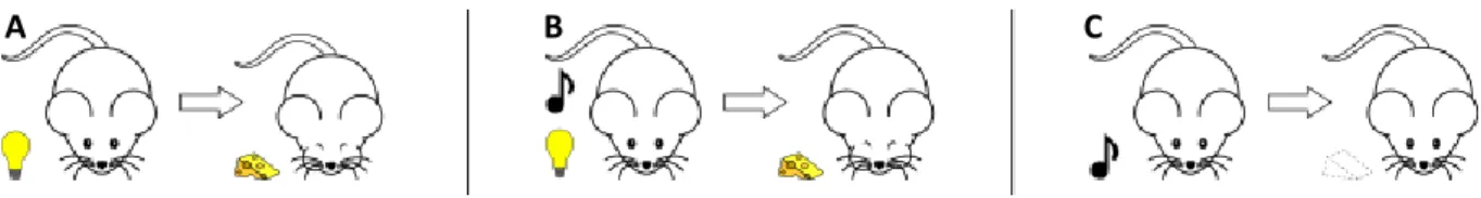
A particular observation was decisive in designing the Rescorla Wagner model which is still a reference today. Kamin describes rat experiments where after conditioning stimulus S1 to reward R (Figure 3 A), a new stimulus S2 is added to S1 and both are paired to R (Figure 3 B). After a new conditioning phase between S1+S2 and R, it is observed on animals that R is not conditioned to S2 alone (Figure 3 C). It means that animals do not look like expecting R when they are presented S2 (Kamin, 1969).

(16)

15

Figure 3: Blocking effect. (A) Light (S1) is associated with food. (B) In a following phase, light (S1) and sound (S2) together are associated with food. (C) Later sound (S2) alone is found not associated with food. From Nicolas Rougier, Blocking, Wikipedia

This result suggests that learning depends critically on the “prediction error”, the difference between what was predicted and what actually happened. Here since R is first conditioned to S1, there is no prediction error when S1+S2 are paired to R, and then S2 do not acquire any predictability of R.

To be comprehensive on this issue, a recent paper, while recognizing the existence and reliability of blocking, contested its universality as they failed to reproduce it in several experiments (Maes et al., 2016).

We will present in the next part the reinforcement model of Rescorla and Wagner.

1.2.1 Rescorla-Wagner model

Rescorla and Wagner published a model accounting for observations on animal learning in particular blocking (Rescorla & Wagner, 1972). It is based on the predictability of reward by an otherwise neutral stimulus, S. When S is repeatedly paired with a reward R, the prediction of R by S will grow until S fully predicts R. Formally it corresponds to a simple equation:

𝑉𝑇+1(𝑆) = 𝑉𝑇(𝑆) + 𝛼 ∗ (𝑅 − [𝑉𝑇(𝑆) + ∑ 𝑉𝑇(𝑂𝑡ℎ𝑒𝑟𝑠) 𝑂𝑡ℎ𝑒𝑟𝑠

]

with 𝑉𝑇(𝑆) the strength of the prediction of R by S at time T. R is the magnitude of the reward (the quantity of reward can vary and can also be zero in case of absence), α is a parameter stable across an experiment measuring the speed of learning, and we include in VT(Others) the possibility that

stimuli happening simultaneously and other than S predicting R, (like S2 in the blocking effect).

Importantly, when the prediction error (here 𝑅 − [𝑉𝑇(𝑆) + 𝑉𝑇(𝑂𝑡ℎ𝑒𝑟𝑠)]) is null 𝑉𝑇+1(𝑆) = 𝑉𝑇(𝑆) and no more learning happens. The prediction error can be seen as a measure of the quality of the prediction VT(S). It is a drive for learning as long as the prediction is not “perfect”.

The strength of the prediction of R by S is named V(S) and is also as stated by the model the

rewarding value acquired by S through learning. Therefore, after learning, animals will like and want S as much as they like and want R as long as the association is maintained.

Interestingly, the concept of prediction error has been biologically validated. A series of work by Wolfram Schultz in Fribourg recorded the response of the dopamine neurons in SNc and VTA. Their activity is qualitatively compatible with a prediction error: It is stronger than baseline in case of unexpected reward, on baseline in case of predicted reward, and under baseline in case the reward is expected but not present (Mirenowicz and Schultz, 1994), (Schultz et al., 1997) (Figure 4).

(17)

16

Figure 4: World famous experience, where midbrain dopamine neurons are recorded in an operant conditioning task. Response transfers from reward to its predictive cue. Absence of reward after learning is perceived as a punition. (Reproduced from (Schultz, Dayan, & Montague, 1997))

It is more difficult to show that this dopamine signal quantitatively match what would be expected by Rescorla Wagner model, as the experiment needs to be perfectly controlled to know precisely what the expected reward is. Experiments validating this idea are more recent but Hannah Bayer & Paul Glimcher showed that at least for positive prediction errors, the dopamine recorded signal

corresponds precisely to what Rescorla Wagner would predict (Bayer and Glimcher, 2005).

It is interesting to note that dopamine neurons are both implicated in the signaling of option values and on the quantification of prediction error. Several computational models of neural circuits in particular in the striatum have accounted for this dual role (Collins and Frank, 2014).

1.2.2 Limits of RW on modeling human data

We showed earlier that the Rescorla Wagner model (RW) explains many human and neuronal data in particular blocking. However, some data cannot be accounted for by RW (Miller et al., 1995). In particular, RW predicts that if after presenting always S and R together (conditioning), S is presented sufficiently alone (extinction), the association between S and R is unlearned and we should go back to the initial situation. However animals display evidence of spontaneous recovery (if extinction is recent, the pairing between S and R can re-emerge without relearning) (Pavlov, 1927), or facilitated relearning (if extinction is recent, re-learning happen faster than initial learning) (Frey and Ross, 1968). These two phenomena are not predicted by the Rescorla Wagner model.

(18)

17

Numerous models have tempted to complicate the RW model to vary the learning equation across time and account for all the limits of RW. To cite only few of them, Wagner itself described a

mechanism where he varied the update equation of the associative strength VT+1(A) in function of the

prior on the strength VT(A) (Wagner, 1981). Mackintosh(Mackintosh, 1975) proposed a model which

tries to identify among all presented stimuli which one is crucial for the reward. Pearce & Hall

introduced a new variable named “salience” applied to the stimulus to modulate learning(Pearce and Hall, 1980). However, due to its simplicity and operational easiness, Rescorla Wagner model is still a reference for the field.

1.2.3 Rescorla Wagner and machine learning

How to learn in a new environment is also major question in the field of machine learning.

Psychology and machine learning have inspired each other during the last decades. Indeed machine learning looks for new ideas in animal learning and computer simulations are an idealized learning environment where the properties of psychological models can be tested. While experimental constraints on animal or human testing prevent from going beyond simple problems like learning by trial and errors, in a virtual environment everything can be adjusted, controlled, repeated; and therefore more complex learning problems can be studied. Thus, algorithms evidenced

experimentally can be tested on more complex situations for generalization. On the converse it is interesting to test whether optimal and complex theoretical algorithms can explain experimental data.

As we saw above, rewards are desirable for a living organism and 2 different rewards can be

compared to each other and ranked by order of preference. Therefore, it is also possible to consider rewards as feedbacks evaluating the quality of the performance. Obtaining 2 apples is “better” than obtaining 1 apple, so it is sensible to bias future choices towards the action which leads to 2 apples. Unfortunately, the behavioral answer to these feedbacks is uncertain as one ignores whether receiving 2 apples is good: there might be an action enabling to win 10 apples!

Therefore, typical problems faced by humans lay between supervised (explicit feedback) and unsupervised (no feedback) learning. They are usually named “Reinforcement learning” problems (Sutton and Barto, 1998). These problems have been transposed in virtual environments, with artificial rewards: the algorithm is rewarded for its actions with points, and it has the instructed goal to maximize his earned points. Models similar to the one of Rescorla Wagner as they use critically the prediction error were developed from the 1950s in machine learning (Minsky and Lee, 1954).

In reinforcement learning problems, the environment is represented as states. In each state,

different actions can be performed. Performing an action can bring some reward, but it also changes the environment so that the following decision will be taken in another state. As an example, to study chess playing, all different configurations of the board can be represented as states. Thus, moving a piece changes the state. Other example, when moving physically from A to B, all positions in between can be considered as states where one can decide to go forward backward right or left.

While navigating the state space, the generic problem is to find the strategy maximizing the total reward received. In particular, some states can be poorly rewarded but lead to very highly rewarded states. This problem generalizes simple operant conditioning cases reported before. There, the credit of a reward was entirely credited to the action which immediately leads to it. Here the entire state-path towards a high reward needs to be credited (Minsky, 1961).

(19)

18

A strategy (or policy) is a probability distribution on the different proposed actions in each of the states. One or several strategies are in average better than the others, but usually all strategies cannot be tried one by one. Indeed if the problem is complex, many successive states are visited in a trial and there are, for example, far more possible chess games than atoms in the universe.

Therefore, reinforcement learning problems are solved by clever exploration methods able to converge in a reasonable time to the optimal strategy.

State of the art methods for reinforcement learning problems are using the concept of prediction error and are named temporal-difference learning (Sutton and Barto, 1981). These methods are particularly easy to implement while being guaranteed to converge to the optimal solution (Sutton and Barto, 1998, p.138).

The principle of these methods is to compute either the value of all states, V(s), either the value of all actions in all states, Q(s,a). V(s) represents the expected future gain when ‘s’ is visited; Q(s,a) the expected future gain when ‘s’ is visited and ‘a’ is performed. These values depend of course on the strategy used. Generally, these methods perform two successive steps in a loop. In a first step the strategy is set and for this strategy, V or Q are computed. In a second step V or Q are used to inform how to modify the strategy in order to increase the earned reward. This defines a new strategy and the first step can be performed once again.

For a given strategy V or Q are computed with a formula similar to the Rescorla Wagner rule. Let’s suppose we are in state S and following the current strategy, action A is performed. This brings a reward r and leads us to state S’. Then V(S) can be updated as,

𝑉_𝑇+1(𝑆) = 𝑉_𝑇(𝑆) + 𝛼 ∗ (𝑟 + 𝑉_𝑇(𝑆′_{) − 𝑉} 𝑇(𝑆))

In the second step, to improve the strategy, one can use directly action values Q(s,a) to increase in each state the probability to choose the action bringing the most reward. Alternatively, state values, V(s) can be used to increase the probability to visit highly rewarded states, but it asks the knowledge of a structural model of the environment: A structural model describes the transition probabilities between states conditioned to actions (p(S->S’|a). This model is independent of the strategy used, and can be learned gradually by experience.

The difference between methods using a structural model and others is central to a long standing debate in animal learning: can animal or human learn and use such a model of the environment? If yes they are said “model-based”, if not “model-free”?

There is an interest in knowing the structural model of the environment when different types of rewards are available and that their relative value varies according to current needs or to time. For example one will not search a house identically if he looks for jewels, or if he looks for the toilets. Without the use of a structural model, any modification in the desirability of rewards asks for the change of all the state-action values and computation of a new optimal policy. On the converse, knowing the structural model allows easy re-planning.

To study the difference between model-based and model-free behavior, a famous paradigm extensively studied in animal psychology is reward devaluation. An action, lever pressing is associated with a food reward (Operant conditioning) then through poisoning or satiety, the

(20)

19

subjective value of the reward is decreased. In a third phase, it is tested whether animals are able to inhibit lever pressing (Figure 5).

In a model free algorithm, the initial action has always been associated with a positive outcome, therefore it still have a high value and is not devaluated. A model based algorithm remembers the arrival state and thus the reward at stake. When the reward is devalued, it can reevaluate action values accordingly and therefore the response will be inhibited.

Figure 5: Usual reward devaluation paradigm: a lever is associated with a food item. This food item is then devaluated. Hypothesis 1: There is a model linking between lever pressing to the food item, then if it does not like the food it does not like also the lever. Hypothesis 2: In the learning phase it transfers the value of the food into the value of the associated lever. It likes the lever but does not “record” why. When the food is devaluated, it still like the lever. From B. Balleine

There are debates to understand whether model free or model based methods are more appropriate to describe human behavior and it seems that there is a part of both (Dayan and Berridge, 2014).

Usual problems in machine learning only use one type of reward, therefore model based and model free algorithms are equivalent. In particular, there is an algorithm able to infer the structural model of the environment from Q(s,a) values: the DYNA algorithm (Sutton, 1990).

Among the model-free algorithms solving reinforcement learning, some are even simpler than temporal difference methods mentioned above as they neither construct nor use a strategy to guide behavior in the different states. One of these algorithms is named Q-Learning and was developed by Watkins during his PhD (Watkins, 1989). This algorithm computes states’ action values Q(s,a) as TD Learning, but these values do not depend on a particular strategy. Instead, in each state the algorithm chooses with high probability the action with the highest value. It cannot always choose the action with the highest value as there is a mathematical constraint on the algorithm to guarantee its convergence to the optimal behavior: every action must be explored sufficiently (the number of times an action is chosen tends to infinity as the number of total trials tend to infinity) (Watkins and Dayan, 1992). Therefore, frequent sub-optimal choices have to be performed in Q-Learning.

In the results of our experimental work, we will compare Bayesian algorithms to model free algorithms and Q-Learning will be our reference.

1.2.4 Theoretical limits of TD LEARNING

TD Learning algorithms in general, Q Learning in particular do minimal hypothesis on the

(21)

20

action values (Watkins and Dayan, 1992). A fundamental limit of these algorithms appears when the environment changes across time. These changes may involve the transition between states (a new street is opened in a neighborhood which modifies itineraries) or the rewarding status of states (one’s favorite restaurant can move or change its cook). TD Learning reacts to a change in the environment by forgetting past Q values, and gradually readapting to the new ones. If a new

environmental change brings the environment back to the initial situation there is no way to retrieve past Q-values.

In particular, our usual environment is seasonal. Winters and summers are very different as the appropriate actions in the two seasons. However, most winters and most summers are similar so that a strategy developed one winter will work the following year. The prediction of TD Learning

algorithms is that Q values will always be relearned from scratch after each change, albeit it would be valuable to retrieve past Q values when the context in which they were valid comes back.

One can imagine that for the same state-action pair, several Q values are memorized in order to account for these different environmental contexts. However, how to decide which set of Q values to use? Which algorithm can manage this selection?

Another limit of TD Learning is its impossibility to generalize its knowledge. If the algorithm learned to play chess, it cannot infer how to play Draught (checkers in American English) and needs to restart its learning from scratch. Indeed a TD Learning algorithm makes no hypothesis on the transition or reward structure of the environment when it starts in a new setting. Yet there are general laws like physical gravity or societal codes which structure most of the situations we face. Therefore, one might expect an efficient learning algorithm to accumulate general information about natural environments which would constitute an a priori strategy when a new setting is encountered. The algorithm would presumably converge faster to the optimal strategy.

Bayesian inference algorithms are an answer to these problems and we will discuss their origin and implementation in the following part.

2. Bayesian Models: Optimal information treatment

2.1. Definition

Bayesian inference is a general statistical method aiming at finding the hidden causes that explain an observation. As an example, when listening at an English speaker (observation), one can guess where he is coming from (what constitutes the “hidden” cause of the accent). To do so, Bayesian inference uses probabilities in order to represent the “belief” or the “confidence” that a particular cause explains the observation. In our former example, the result of the Bayesian analysis can, for example, be that the speaker has 30% chance of being Spanish, 50% of being French and 20% of being Italian.

When they were introduced, Bayesian statistics were a new use of probabilities as probabilities were initially only used to represent known frequencies. The name “Bayesian” refers to Thomas Bayes who proposed a formula to compute the now called beta distribution: a distribution of the probability of success at a lottery given the number of successes so far (Bayes and Price, 1763). This approach was formalized and popularized later by Pierre-Simon Laplace who gave a formulation of what is now named Bayes Theorem (Laplace, 1774).

(22)

21

𝑝(𝑐𝑎𝑢𝑠𝑒_𝑖|𝑜𝑏𝑠) = 𝑝(𝑜𝑏𝑠|𝑐𝑎𝑢𝑠𝑒𝑖) ∗ 𝑝(𝑐𝑎𝑢𝑠𝑒𝑖) ∑ 𝑝(𝑜𝑏𝑠|𝑐𝑎𝑢𝑠𝑒𝑗 _𝑗) ∗ 𝑝(𝑐𝑎𝑢𝑠𝑒𝑗)

Therefore, given an observation, the probability that a cause (i) is responsible for the observation can be inferred from knowledge of how likely all possible causes (j) would generate this observation.

What is particularly interesting is the possibility to build up on it when a new independent observation (obs_new) is acquired.

𝑝(𝑐𝑎𝑢𝑠𝑒𝑖|𝑜𝑏𝑠, 𝑜𝑏𝑠_𝑛𝑒𝑤) =

𝑝(𝑜𝑏𝑠_𝑛𝑒𝑤|𝑐𝑎𝑢𝑠𝑒_𝑖) ∗ 𝑝(𝑐𝑎𝑢𝑠𝑒_𝑖|𝑜𝑏𝑠) ∑ 𝑝(𝑜𝑏𝑠_𝑛𝑒𝑤|𝑐𝑎𝑢𝑠𝑒𝑗 _𝑗) ∗ 𝑝(𝑐𝑎𝑢𝑠𝑒𝑗|𝑜𝑏𝑠)

The independence of the two observations, obs and obs_new enables to use the result of the former computation, 𝑝(𝑐𝑎𝑢𝑠𝑒𝑖|𝑜𝑏𝑠), as a prior for the latter, and this can go on as new information are added. This process makes this method particularly appropriate to data acquired sequentially, where intermediate decisions have to be taken in parallel to data acquisition.

Using probabilities to represent beliefs and combine them through Bayes theorem has been shown by Cox’s theorem to correspond to what one can expect from an optimal “logical” reasoning system (Cox, 1946), (Van Horn, 2003). Therefore, Bayesian inference refers as a good paradigm to reason in an uncertain environment, and consequently is a good hypothesis to explain how the brain could perform probabilistic learning (Tenenbaum et al., 2011).

2.2 Principles of Bayesian inference

Bayesian inference can be used to model almost everything. However, three elements need to be defined to use it properly:

- The ensemble of causes: A set of possible causes well identified must be defined. Causes represent “hidden states”, in the sense that they are not directly observable but that they still influence observations. It is the goal of the inference to find the hidden state that explains observations the best. In the previous example where one has to guess the origin of an English accent, causes can be nationalities, mother tongues, social origin, etc. However, it can also be the combination of several of them (one exemplar cause would then be: popular Brazilian with Hebrew as a mother tongue). The more causes there are, the more precise the result is (popular Brazilian is more precise than just Brazilian), but the more computations have to be performed to track the likelihood of all causes.

- A likelihood function for each of the causes: The definition of the ensemble of causes is crucial as for all possible causes “j”, and for all observations, it is necessary to know 𝑝(𝑜𝑏𝑠|𝑐𝑎𝑢𝑠𝑒𝑗): how likely is the observation knowing cause “j”. This knowledge allows for comparing the likelihood of an observation given different causes. In the example given above (determine the origin of someone according to his accent), the likelihood function allows generating English as spoken by all

nationalities considered as possible causes. The likelihood function integrates a huge quantity of information and learning it is usually a major difficulty which can prevent the use of Bayesian inference.

In the example of Thomas Bayes, the likelihood function is trivial. Indeed, for all p, the probability to win at a lottery which has a probability p is p. In machine learning applications, the likelihood

(23)

22

function is complex but will often be given to algorithms as an input. However, for behavioral

application, the key question is to understand how brains acquire and represent likelihood functions.

-The prior: The last key element for Bayesian inference is to have a prior probability distribution on the different causes: before seeing any observation, what is a priori the current hidden state? First, observations will be combined with the prior to give a posterior probability distribution on the causes, which will serve as a prior for later acquired observations. The prior can be freely chosen albeit using accurate priors is critical in particular when there is little information in observations. In the English accent example, the prior can be the probability to meet each of the possible nationalities in the present context. An alternative would be to compute priors through another inference on the visual look of the speaker. If no relevant information is available, the prior can also be defined as uniform on the different possible causes. In all cases the prior influences the final result: if one expects someone to be Spanish and not Italian, and that at the same time his accent is ambiguous, he will be classified as Spanish. And the converse if the speaker is expected to be Italian despite the observation is identical.

Thomas Bayes used a uniform prior on the probability of success at a lottery, what was a posteriori justified by Laplace as being the best prior to use when no information is available.

The combination of the likelihood function and the prior constitutes a generative model. It includes all the information about the environment. Thus, the generative model allows a complete simulation of the environment in particular the generation of fictive observations.

In its formula, Bayes theorem gives the same weight to both the prior and the likelihood function. Therefore, the posterior distribution is driven by the more precise of these two functions. Thus, if priors are non-informative (for example a uniform prior), then posteriors will follow the likelihood function, and if observations are non-informative according to the likelihood function (equally likely for every cause), then the posteriors will be aligned to priors. The Bayesian formula accounts for uncertainty and favors sure sources of information.

To illustrate the power of the approach, there are cases where a little observation is revealed through the generative model as crucial information. For example, if Australians have a specific way of pronouncing “y”, only hearing a single word with a “y” is sufficient to be sure that the speaker is Australian. Past information has been stored in the generative model (priors and likelihood function) and Bayesian inference uses this knowledge to interpret efficiently any new observation.

Bayesian inference has been proposed to be the solution used by the brain to deal with multiple uncertain sources of information (Pouget et al., 2013). In the next part, we will go through available evidence validating this hypothesis.

2.3 Bayesian inference and human behavior

2.3.1 Perception

Since the end of the 19th century, scientists have proposed that human perception can be described by Bayesian inference (Mach and Williams, 1897). Indeed Bayesian inference answers to a

fundamental problem of any perceptual system. Perception relies on receptors which sense information on dimensions which are not the one on which information will be eventually

(24)

23

relevant information is the image that they code. This poses an inverse problem: what is in the space of all possible images the most likely cause of the data coded by the receptor.

In particular, when information is compressed by the receptor, there will be several possible causes to the data and the inverse problem is underdetermined. To solve this issue, priors based on habitual scene structure or previous images will limit the number of possible interpretations of data and constrain interpretation towards the “good” one.

Bayesian algorithms have been developed in the 1980s to create an artificial visual system (Bolle and Cooper, 1984). These approaches were later demonstrated appropriate (Kersten, 1990) and

successful (Bülthoff and Mallot, 1988), (Knill and Richards, 1996) at modeling human visual system.

Furthermore Bayesian inference has been evidenced to describe optimal information combination that happens between different human perceptive systems. Van Beers & colleagues showed that when two different sources of perceptive information are integrated, the weighting between the two in the final representation depends upon their relative precision. This constitutes the core of Bayes theorem (van Beers et al., 1999). Quantitative account of this weighting was demonstrated by Ernst & Banks in a visual/haptic combination (Ernst and Banks, 2002).

2.3.2 Abstract reasoning

The use of Bayesian algorithms has not only been reported at the perceptual level. The prefrontal cortex, which operates complex and abstract reasoning in human, has been described as following Bayesian inference rules. Collins & Koechlin have proposed a Bayesian model of reasoning, where an algorithm integrates information across time to find the current hidden state of the world and select accordingly the best available action. Their model treats information optimally except for an account of human memory and computational limitations (Collins and Koechlin, 2012). Neural correlates of the model evidencing a use of probabilistic reasoning have been found with functional Magnetic Resonance Imaging (fMRI). In particular, parts of the prefrontal cortex track the likelihood of the different possible hidden states (Donoso et al., 2014).

To continue on high level reasoning and abstract causes, most social behavior of individuals constitute as well a natural field where Bayesian inference principles can be applied. Indeed social interactions rely on the understanding of intentions of others. Understanding others allows an adequate interpretation of their behavior and therefore an appropriate reaction. Intentions can be considered as hidden states that behavioral and contextual observations help to determine. For example, the sentence “Do we have to do this?” can be interrogative or complaining. To react appropriately, one can either use the tone with which the sentence was pronounced, or the facial emotion displayed when it was pronounced, or both.

In general this ability to decode others intentions is named theory of mind (Premack and Woodruff, 1978). Baker, Saxe & Tenenbaum proposed a Bayesian model of the use of others’ actions to understand their beliefs and desires(Baker et al., 2011). The authors confirmed their model experimentally and showed that human data fit to model predictions and are therefore close to optimal rational behavior. Similar optimality results were found in economic games bearing uncertainty on the intention of other actors (McKelvey and Palfrey, 1992), or on tasks where language ambiguities have to be decoded (Jurafsky, 1996).

(25)

24

These multiple examples of brain mechanisms which can be modeled by Bayesian algorithms suggest it is a general information treatment mechanism in the brain. The resulting questions are 1/whether it is possible for neurons to encode probability distributions and to apply simply the Bayes theorem, and 2/are there neuronal evidences that it is happening?

2.3.3 Neuronal implementation of Bayesian inference

Instead of a fixed value, several authors have proposed that neurons could encode the probability (Anastasio et al., 2000), or the log-probability (Barlow, 1969) of an event. The coding in log

probability is particularly interesting as multiplications in Bayes theorem become summations and are simpler to perform neuronally.

Alternatively, it is also possible to encode full probability distributions at the neuronal population level. Indeed, when several noisy neurons encode the same variable, the resulting activity of the population can be interpreted as a probability distribution over this variable (Zemel et al., 1998). Noisy representations of variables have particular properties which make them particularly suited to neuronal combination and Bayesian inference is easy to perform with population codes (Ma et al., 2006). Neural correlates of a Bayesian combination of population codes were found in neuronal recordings of monkeys (Fetsch et al., 2011).

Another different way to easily perform Bayesian inference with neurons is to mimic Monte Carlo methods. Indeed, each neuron of a population can be seen as coding a drawing (sample) of a distribution. Bayes theorem will then apply to all the individual samples to obtain eventually a sampled representation of the posterior distribution (Hoyer and Hyvarinen, 2003).

To justify the presence and the evolutionary maintenance of Bayesian inference in the brain, we presented that beyond perceptual problems, Bayesian inference allows complex abstract reasoning and is crucial in social contexts. It indeed allows individuals to understand each other in a group and is then decisive for social cohesion. A major hypothesis in evolution explains the development of higher cognitive abilities and “intelligence” as an evolutionary pressure due to the social challenges to live in a group (Jolly, 1966), (Humphrey, 1976). As an example, not understanding the negative intention of a pair diminishes the individual survival chances. On the contrary, overestimating negative intentions may lead to anti-social behavior and to an exclusion from the group. Exclusion also diminishes chances of survival. With this hypothesis, sophisticated problem solving capacities (like chess playing) would be a by-product of social abilities needed to understand others (Dunbar, 1998).

After this presentation, major questions are still remaining: Bayesian inference describes how priors and likelihood functions are combined after an observation, but does not tell whether these two basic elements are innate or acquired. Thus, if they are innate why are they evolutionarily relevant and to which implicit hypotheses on the world are they equivalent to? And if they are acquired, what is the acquisition mechanism?

(26)

25

2.4 Learning a generative model

2.4.1 Comparison of human performance and state of the art algorithms

Amongst the many applications of Bayesian inference, the problem of learning generative models came from studies on how children learn language. The scientific study of language is inherited from Quine and can be presented as an induction problem (Quine, 1960). Indeed children have to use the adequate word, which can be seen as a hidden state, given the situation. The classical observation is that humans are very good at word learning and a few labeled examples are enough to generalize to other instances of the category (Xu and Tenenbaum, 2007).

This is considered as exceptional and impossible to reproduce on artificial learning systems. Indeed, when only a few examples of a word are presented, there are necessarily ambiguities. For example to learn what is a “dog”, only some breeds of dogs will be shown, so the learner has to interpret by itself that “4 legged animals” is too wide and “Dalmatians” is too narrow. Experimental evidence shows that humans perform this task correctly (Carey, 1978).

Human performance outperforms all computer algorithms on word learning or classification tasks. In one example, humans and algorithms had to learn the name of 256 objects. After learning, humans recognized 56% of objects (Eitz et al., 2012), while the best algorithm was at 33% (Borji and Itti, 2014).

It can be argued that humans are favored in this task as they already know thousands of words and can therefore use this prior knowledge to ease learning. François Fleuret and colleagues then designed an inference based scene classification task with abstract images so that prior knowledge was irrelevant and could not be applied. After a few examples, humans and computers had to classify abstract test images in different categories. With 20 exemplar images humans were able to solve most of the problems, while computers were at chance level. Computers needed 10’000 examples to solve some of the problems and their performance was still not close to human performance (Fleuret et al., 2011).

In this task, Bayesian inference computes 𝑝(𝑐𝑎𝑡𝑒𝑔𝑜𝑟𝑦 | 𝑖𝑚𝑎𝑔𝑒) thanks to the generative model 𝑝(𝑖𝑚𝑎𝑔𝑒 | 𝑐𝑎𝑡𝑒𝑔𝑜𝑟𝑦). Since images and categories are abstract, the generative model is learned only during the presentation of labelled images. How human can be so efficient in this learning? Understanding it is a challenge for Psychology and has potential applications in machine learning and robotics.

In the case of language as in any learning setting, the generic problem is that there are many candidate categories which would match with provided examples and all possibilities cannot be tested exhaustively. The problem is underdetermined. Braun & al describe how the human mind could solve this issue and they illustrate their intuition by a parallel with a simple example in motor learning (Braun et al., 2010).

To produce a target movement, all muscles and all articulations could theoretically be used in all their degrees of freedom. However, only a limited combination of muscles and articulations produce a meaningful action and limiting exploration to this subset accelerates the finding of the correct movement. It is the same when an animal on a picture is named “dog”. A huge number of implicit assumptions about scene organization, pointing, and animal generic definition limit the set of

(27)

26

regularities which will be associated with the “dog” category. Without these assumptions, as for machine learning algorithms, a lot of images would be needed to constrain sufficiently the interpretation to a unique well-specified category.

Generic assumptions about the environment can be learned on a longer time scale and are not specific to a particular learning problem. They eventually capture the implicit and explicit structure of the environment and can be used to constrain any subsequent learning to the smallest solution space where these assumptions are valid.

To illustrate the interest and the potential advantages of structure learning, a machine learning team at Google used their super powerful calculators to find regularities on millions of random images picked from the internet (Le et al., 2013). This can be seen as analog to a young child looking around him for several years. The algorithm is an unsupervised neuronal network and after training each neuron responds to one of the spotted regularities. A few labeled images of say human faces were then presented to the algorithm. This is analog to a child who would be presented with a few exemplar images of a new category. Among all neurons of the net, some were responding particularly well to the human faces presented. These neurons were selected and new images (human faces and other unrelated images) were later presented to the network. The main result is that these selected neurons were detecting reliably human faces. Critically only a few labeled images were presented to the algorithm, what is far less costly to produce than the 10,000 labeled images that would have been needed without the first phase of unsupervised learning. This is a method of self-taught learning (Raina et al., 2007), which proves the validity of the concept of structure learning. In the case of natural images structure represents for example contours, principal colors, usual shapes…

2.4.2 Hierarchical Bayesian models

The algorithm used by the Google team is well understood, but it is interesting to understand how the brain routinely extracts structure all along life. One influential hypothesis proposes the use of Bayesian inference and in particular, hierarchical Bayesian models at this end (Tenenbaum et al., 2011). The general idea is that on very long time scales, knowledge is accumulated to learn how to spot statistical regularities (causal models (Tenenbaum and Griffiths, 2001a)) and how to

appropriately transfer knowledge from one problem to the other (generalization (Tenenbaum and Griffiths, 2001b)). Indeed there are always different ways to generalize, or different types of causal structures. Evidence is accumulated to select in a particular environment the appropriate

generalization and causal structure. At a lower hierarchical level, these structures are applied to the building of the current generative model which can be tuned faster.

For example, in animal naming, a natural structure is to separate ground animals from flying animals from sea animals. Then among ground animal, separate oviparous from mammals. Then among mammals, bipeds from quadrupeds; among quadrupeds, urban, savannah and forest animals. Among urban animals, dogs, cats, etc.

When several examples are shown to instruct a new category, localizing these examples in the pre-learned structure enables to extract easily what is the general category that needs to be named (Xu and Tenenbaum, 2007). The generalization is also immediate: if a property is shared by several ground mammals, it is reasonable to generalize the property to all of them.