HAL Id: hal-00960670
https://hal.archives-ouvertes.fr/hal-00960670
Submitted on 18 Mar 2014HAL is a multi-disciplinary open access
archive for the deposit and dissemination of sci-entific research documents, whether they are pub-lished or not. The documents may come from teaching and research institutions in France or abroad, or from public or private research centers.
L’archive ouverte pluridisciplinaire HAL, est destinée au dépôt et à la diffusion de documents scientifiques de niveau recherche, publiés ou non, émanant des établissements d’enseignement et de recherche français ou étrangers, des laboratoires publics ou privés.
Direct numerical simulations for smouldering in
horizontal channel
Chen Yang, Gérald Debenest
To cite this version:
Chen Yang, Gérald Debenest. Direct numerical simulations for smouldering in horizontal channel. Eighth Mediterranean Combustion Symposium -, Sep 2013, Izmir, Turkey. �hal-00960670�
O
pen
A
rchive
T
OULOUSE
A
rchive
O
uverte (
OATAO
)
OATAO is an open access repository that collects the work of Toulouse researchers and makes it freely available over the web where possible.This is an author-deposited version published in : http://oatao.univ-toulouse.fr/
Eprints ID : 11198
To cite this version : Yang, Chen and Debenest, Gérald Direct
numerical simulations for smouldering in horizontal channel. (2013) In: Eighth Mediterranean Combustion Symposium - , 08 September 2013 - 13 September 2013 (Izmir, Turkey)
Any correspondance concerning this service should be sent to the repository administrator: [email protected]
DIRECT NUMERICAL SIMULATIONS FOR SMOULDERING
IN THE HORIZONTAL CHANNEL
C. Yang* and G. Debenest
IMFT, Allée Camille Soula, F-31400 Toulouse, France
Abstract
In the present study, direct numerical simulations for smouldering in a horizontal channel are performed for both compressible and incompressible flows. The reactant gas is passing through the char surface, where the chemical reaction is going to take place. For the sake of simplicity, the smouldering is treated to be a single step chemical reaction. In the incompressible flow, a set of governing parameters are discussed to elucidate their influences on the process of smouldering. Furthermore, the variations of density and dynamic viscosity of gaseous mixture are taken into account in the compressible flow. The comparison between the compressible and incompressible flows reveals that the effects of local compressibility and gaseous mixture on the propagation of smouldering wave are trivial.
Introduction
Smouldering is the flameless combustion of a liquid or solid fuel that derives heat from surface oxidation reactions. In a porous material, the local pore structure allows gaseous reactant to filter through the solid to the reaction site. Substantially, the smouldering wave can propagate through the interior of porous media sample. Due to its vast potential applications, such as porous media burner, waste incineration, catalyst regeneration, oil recovery enhancement and many others applications [1-3], smouldering in porous media has attracted a lot of interests.
In the open literature, tremendous number of publications relevant to the smouldering in porous media can be found. Aldushin et al. [4] started a pioneering work by conducting the one-dimensional theoretical analysis of combustion propagation wave in a porous media. Based on the asymptotic method, structure of solution was determined for the first time. For two different structures, Schult et al. [5] discussed solutions for reaction leading and reaction trailing wave structures by virtue of asymptotic method. A so-called reaction leading structure occurs when the velocity of combustion front overcomes that of the heat transfer layer. On the contrary, the velocity of combustion front is slower than that of the heat transfer layer in the reaction trailing structure.
Regarding to the numerical simulations in the microscope geometry of porous media, two simple structures, which are array of horizontal channels and staggered cylinders, are usually utilized for the computational analysis. Debenest et al. [6] proposed a three-dimensional microscale numerical model for the simulation of smouldering in fixed beds of solid fuels. In light of a dimensional analysis, Debenest et al. [7] identified a set of governing parameters. Furthermore, direct and detailed numerical simulations on the microscale were performed to elucidate their influences.
However, to our best knowledge, no microscale calculations associated with the smouldering in a porous media have been done yet in the compressible flow. In this study, the smouldering in the array of horizontal channels shall be revisited to investigate the effects of a set of governing equations for the incompressible flow. Then, based on the same geometry, we shall consider the variations of density and dynamic viscosity of gaseous mixture to discuss the local effects of compressibility and gaseous mixture in the compressible flow.
Mathematical Model and Governing Equations
As illustrated in Fig 1(a), the gas is passing through the array of horizontal channels. The gray part is the char for combustion, and the other part is the passage for gas. The smouldering, which is simplified to a single step chemical reaction, is going to take place in the interface between these two parts. Due to the periodicity of geometry, a unit cell would be good enough to capture the characteristics of smouldering. Moreover, for the sake of simplicity, the half of a unit cell shown in Fig 1(b) is chosen for the calculations in this study.
Figure 1(a). Horizontal channels.
Figure 1(b). Calculation domain.
Based on the mathematical model given by Debenest et al. [6], the governing equations used in this study for incompressible flow are indicated as following:
( )
=
0
⋅
∇
+
∂
∂
u
t
ρ
ρ
(1)( )
u p u u t u+ ⋅∇ =−∇ + ∇2 ∂ ∂ρ
ρ
µ
(2)0
2 2+
∇
⋅
=
∂
∂
O OJ
t
c
(3a) 2 2 2 2 O O O O uc D c J = − ∇ (3b)(
)
0
=
⋅
∇
+
∂
∂
Tg g gJ
t
T
C
(4a)J
Tg=
C
guT
g−
λ
g∇
T
g (4b)(
)
0
=
⋅
∇
+
∂
∂
Ts s sJ
t
T
C
(5a)J
T sT
s s=
−
λ
∇
(5b)where
2 o
c is the concentration of oxygen, Tgand T are the temperature of gas and solid s
phases, respectively. Moreover, C and g C are the volumetric heat capacities for gas and s
solid phases.
Correspondingly, the boundary conditions for incompressible flow are set as follows: For t = 0 and inlet:
in u u = , Tg =Ts =500K and 3
376
.
8
2mol
m
c
O=
(6) For t = 0 and outlet:0 2 = ∂ ∂ = ∂ ∂ = ∂ ∂ = ∂ ∂ x c x T x T x u g s O (7) Whereas the interfacial conditions between two phases are given by:
s m u=0 / , Tg =Ts,
n
⋅
(
J
Tg−
J
Ts)
=
∆
h
cn
⋅
J
O2 (8) 2 2 O OS
J
=
⋅
n
and J ds dt dc g O g c∫
∂ ⋅ − = υυ
2 1 nwhere
c
c is the concentration of char,∆
h
c is the carbon-oxygen heat of combustion,υ
g is the grain volume,∂
υ
g is its surface andds
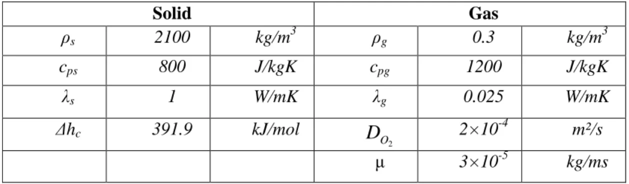
is a surface element.Furthermore, the properties used in the incompressible flow are listed in Table 1.
Table 1. Properties in the incompressible flow
Solid Gas ρs 2100 kg/m3 ρg 0.3 kg/m3 cps 800 J/kgK cpg 1200 J/kgK λs 1 W/mK λg 0.025 W/mK ∆hc 391.9 kJ/mol 2 O
D
2×10⁻⁴ m²/s µ 3×10⁻⁵ kg/msIn the incompressible flow, all properties of both gas and solid phases are kept to be uniform and constant. However, in the compressible flow, the variations of density and dynamic viscosity of gas phase are considered in the present study. In addition, the incoming gas is the mixture of oxygen and nitrogen in compressible flow rather than a tracer approximation for oxygen in the incompressible flow. Owing to the utilization of single step chemical reaction, the generation of carbon dioxide is also considered in the compressible flow.
Based on the difference between the compressible and incompressible flows as described above, the governing equations associated with the compressible flow modified from equations (1) ~ (5) are presented as below:
0
=
⋅
∇
+
∂
∂
ρρ
J
t
(9a) Jρ =ρ
u (9b)( )
u p u u t u+ ⋅∇ =−∇ + ∇2 ∂ ∂ρ
ρ
µ
(10)0 2 2 2 +∇⋅ = ∂ ∂ O W O J t M Y O
ρ
(11a)(
)
2 2 2 2 2 O O O WO OuY
D
Y
M
J
=
ρ
−
ρ
∇
(11b)0
2 2 2+
∇
⋅
=
∂
∂
CO W COJ
t
M
Y
COρ
(12a)(
)
2 2 2 2 2 CO CO CO WCO COuY
D
Y
M
J
=
ρ
−
ρ
∇
(12b) 2 2 21
O CO NY
Y
Y
=
−
−
(13)(
)
0
=
⋅
∇
+
∂
∂
Tg g gJ
t
T
C
(14a)J
Tg=
C
guT
g−
λ
g∇
T
g (14b)(
)
0
=
⋅
∇
+
∂
∂
Ts s sJ
t
T
C
(15a)J
T sT
s s=
−
λ
∇
(15b)where the Y is the mass fraction of pure gas, and the variations of density and dynamic i
viscosity of gas phase are achieved by the following two equations:
(
)
∑
= = N i i W g uT Y M i R p 1ρ
(16) and i N i Xiµ
µ
=∑
=1 (17) where R is the universal gas constant, u MWi and Xi are the molecular weight and molarfraction of pure gas, respectively. In addition,
µ
i is the dynamic viscosity of pure gas which can be calculated as follows:2 1 g g B g i T D T C AT + + =
µ
(18) The corresponding coefficients for the pure gas in equation () referred from Chapman and Cowling [8] are listed in Table 2.Table 2. Coefficients in the equation ()
A B C D 2 O 1.10×10⁻⁶ 0.56 96.3 0 2 CO 2.14×10⁻⁶ 0.46 290 0 2 N 6.56×10⁻⁷ 0.61 54.7 0
Correspondingly, the boundary conditions for compressible flow are set as follows: For t = 0 and inlet:
in u u = , Tg =Ts =500K, 2 O
Y
= 0.8935, 0.1787, 0.0596, 0 2 = CO Y , 2 2 21
O CO NY
Y
Y
=
−
−
(19)For t = 0 and outlet:
0 2 2 2 = ∂ ∂ = ∂ ∂ = ∂ ∂ = ∂ ∂ = ∂ ∂ = ∂ ∂ x Y x Y x Y x T x T x u g s O N CO (20)
Whereas the interfacial conditions between two phases are given by: s m u =0 / , Tg =Ts,
(
)
2 O c s T TJ
h
J
J
g−
=
∆
⋅
⋅
n
n
, 2 2 O OS
J
=
⋅
n
, (21) 2 2 2 2 2 CO O WCO WO CO S S M M J = = × ⋅ n , 2 2 O CO S S S J = = − ⋅ ρ ρ n J ds dt dc g O g c∫
∂ ⋅ − = υυ
2 1 nIn the present study, a set of governing parameters used for the analysis are presented as follows: O B
D
W
u
Pe
=
, 2 O s c gc
C
c
C
∆
∆
=
∆
, s s g g c c s adC
C
h
c
T
ε
ε
ε
+
∆
∆
=
,1
−
∆
=
ad pT
T
(22a, b, c, d)where εg and
ε
s are porosities of gas and solid phases, Tad and T are the adiabatic ptemperature and plateau temperature, respectively.
Code Validations
The foregoing sets of governing equations are solved numerically by using the OpenFOAM Version 2.1.1 package. Since the process of smouldering is transient, PIMPLE algorithm designed for the large time-step computations is chosen to be the numerical scheme. The transient terms of the foregoing sets of governing equations were discretized using the first order Euler implicit scheme. For the convergence criteria, the residuals of all variables are less than 10-12. Moreover, we have performed a sensitivity analysis to the grid size. Then, all of the calculation results in the present study are independent of the grid size.
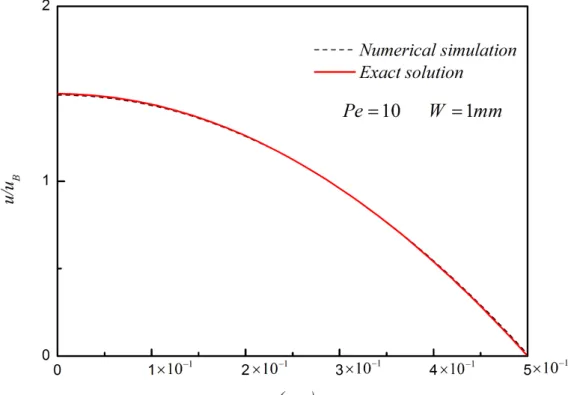
As depicted in Fig 2., the fully developed velocity profile of cross-section in the channel is compared with the corresponding exact solution. It can be seen that the agreement between two velocity profiles is good. According to the prediction of Debenest et al. [7], the transversally averaged temperature is supposed to reach the plateau temperature calculated by equation (22d). In Fig. 3., the transversally averaged temperature comes to the plateau temperature when the location of combustion front is 70W.
Figure 3. Profile of the transversally averaged temperature in the horizontal channel
Results and Discussion
Several tests were made in order to check the accuracy of the model. They are all summarized in Table 3.
For all the calculations, Pe and ∆, we report in Table 3 are the results obtained for averaged temperature divided by the adiabatic one. If the results are correct, it will normally converge to the value of 1 ∆−1 , according to Aldushin et al. [4]. We can see a good agreement with the theory for Pe = 1, 10; ∆ = 0.1 with a profile of averaged temperature coming to the expected temperature. But, for ∆ values equal to 0.5 and 1.5, less than 3% of difference is observed. This is the asymptotic value reached numerically and several things could explain that. Main direction we have today, is the grid size in y direction as the reaction term depends strongly on the concentration of oxygen. This will be investigated in a forthcoming paper. But as evidence, we can consider that the numerical tool is valid, and could be a starting point for further investigations. We are now going to see more in details of the results.
As illustrated in Fig 4., Fig 5. and Fig6., profiles of transversally averaged temperature of gas and solid phases are presented for three different ∆. The Peclect number, Pe, is kept constant and equal to 10. Different ∆ can be interpreted as different char concentration in the solid or different oxidizer concentration in the gas. In these three figures, it can be clearly seen that the smouldering wave propagates as the time goes by, and eventually comes to the steady regime. This time depends on the flow regime as seen in Debenest et al. [7].
Table 3. Several cases in the present study
Pe ∆ 0.1 0.5 1.5
Tp/Tad
Numerical Analytical Numerical Analytical Numerical Analytical
1 1.11 1.111 2.0 2.0
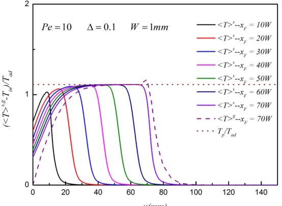
Figure 4. Profiles of the transversally averaged temperature of fluid and solid phases for
1 . 0
=
∆ and Pe=10 in incompressible flow.
In the Fig. 4., the steady regime is obtained after 40 W. We can see a difference in the averaged temperature profiles between gas and solid phase. At the inlet, the gas phase needs several W before being at the equilibrium with the solid phase. A peak is observed in the gas phase, in the reaction region. Then, the gas phase appears to be hotter than the solid phase. This is due to the convective part in the equation (4a).
Figure 5. Profiles of the transversally averaged temperature of fluid and solid phases for
5 . 0
=
In the Fig. 5., the steady regime is obtained after 160 W. The maximum averaged temperature is really closed to the one expected. We also observe that the heat content stays closer to the reaction region than in the previous case. This is coming from the increasing ∆ value. Heat velocity is now closed to the reaction front velocity and the two waves propagate at nearly the same speed.
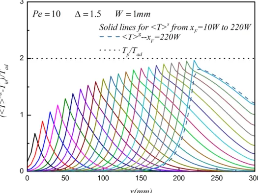
In the figure 6, the steady regime is obtained after 220W. The maximum temperature is closed to 2Tad. The thermal wave propagates quicker than the reaction wave, so the heat content accumulates after the reaction region.
In these last two cases, we see the same differences in averaged profiles between gas and solid phases than in figure 4. The convective part of equation (4a) explains once again this effect comment could be done. This is in agreement with the results of Debenest et al. [7]. But we present there the first local approach reaching the steady regime expected.
Figure 6. Profiles of the transversally averaged temperature of fluid and solid phases for
5 . 1
=
∆ and Pe=10 in incompressible flow.
In Fig. 7, the case Pe = 1; ∆ = 0.1 is given. After 50W, the steady regime is observed and the averaged temperature reaches the expected value. When the combustion front comes to 70W, the averaged profiles of gas temperature and solid temperature are plotted. No significant differences exist, except in the inlet zone, where the gas phase enters at 500K. In the front region, a peak temperature exists in the gas phase. This comes from the reaction at the interface. Then, the gas temperature releases to the solid temperature. The same ∆ value with a Pe = 10, gives us a strong difference in space between the two temperatures. Because of the small value of Pe and especially of thermal Pe value like explained in Debenest et al. [9], in this case no differences are seen.
Let’s go now to the compressible flows as introduced in equation (9) to (15). The last part of this paper will be dedicated to the comparison between incompressible and compressible flows and quantification of the effects of composition and temperature with density and dynamic viscosity. Several tests will be made to compare with our incompressible case by varying Pe number, intensive and further investigation of ∆ values will be addressed in a coming paper.
Figure 7. Profiles of the transversally averaged temperature of fluid and solid phases for
1 . 0
=
∆ and Pe=1 in incompressible flow.
In the Fig. 8 and Fig. 9, the cases of Pe = 1 and 10 for the ∆ = 0.1 are presented in the
compressible flow. By comparing these two figures with Fig. 4. and Fig. 7, it can be seen that the variations of density and dynamic viscosity of gas phase have no remarkable influences on the propagation of smouldering wave. The further investigations seem to be necessary, such as more accurate chemical reaction schemes, variation of thermal capacity of gas phase, etc.
Figure 8. Profiles of the transversally averaged temperature of fluid and solid phases for
1 . 0
=
Figure 9. Profiles of the transversally averaged temperature of fluid and solid phases for
1 . 0
=
∆ and Pe=1 in compressible flow.
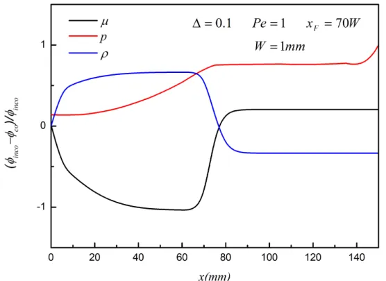
As shown in the Fig. 10 and Fig. 11, the difference of pressure, density and dynamic viscosity of gas phase between the compressible and incompressible flows are plotted in the direction of smouldering wave propagation. The comparison results clearly indicate that the difference is significant; especially in the chemical reaction region. This is because the variations of density and dynamic viscosity of gas phase are highly temperature-dependent.
Figure 10. Comparisons between the compressible and incompressible flows for ∆=0.1 and 10
=
Figure 11. Comparisons between the compressible and incompressible flows for ∆=0.1 and 1
=
Pe
Conclusions
In the present study, direct numerical simulations were made to investigate the effects of a set of governing parameters on the smouldering process in a horizontal channel. The calculations were carried out for both compressible and incompressible flows. In the incompressible flow, it was found that a so-called reacting leading structure appears for ∆ < 1, and ∆ > 1 results in the reacting trailing structure. Moreover, it also should be noted that for the same ∆, the case of Pe = 1 has smaller temperature difference between the gas and solid phases than that of Pe
= 10 does, which implies that the local thermal equilibrium assumption could be valid in the case of Pe = 1. By varing the density and dynamic viscosity of gas phase, the calculations
were conducted in the compressible flow to discuss the effects of local compressibility and gaseous mixture on the propagation of smouldering wave. The comparison between the compressible and incompressible flows demonstrates that the variations of pressure, density and dynamic viscosity of gas phase in the direction of smouldering propagation wave are significant. However, the effects of local compressibility and gaseous mixture on the propagation of smouldering wave are negligible.
Nomenclature
c concentration
C volumetric heat capacity D diffusivity of pure gas
hc carbon-oxygen heat of combustion
J flux
MW molecular weight
p pressure Pe Pelect number
Ru universal gas constant
T temperature u velocity
W height of gas passage x, y Cartesian coordinates X molar fraction Y mass fraction ε porosity λ thermal conductivity µ dynamic viscosity
ρ
density Subscripts ad adiabatic c char B bulk F combustion front g gas in inlet O2 oxygen N2 nitrogen CO2 carbon dioxide p plateau s solid Superscripts g gas s solid References[1] Sarathi, P. S., In-situ combustion handbook—principles and practices, Tulsa, 1999. [2] Ohlemiller, T. J., “Modeling of smouldering combustion propagation”, Prog. Energy
Comb. Sci. 11: 277-310 (1985)
[3] Oliveira, M., Kaviany, M., “Nonequilibrium in the transport of heat and reactants in combustion in porous media”, Prog. Energy Comb. Sci. 27: 523-545 (2001)
[4] Aldushin, A. P., Merzhanov, A. G., Seplyarskii, B. S., “Theory of filtration combustion of metals”, Fiz Goren Vzryua 12: 323-328 (1976)
[5] Schult, D. A., Matkowsky, B. J., Volpert, V. A., “Forced forward smolder combustion”,
Eng. Sci. 2180: 1-26 (1996)
[6] Debenest, G., Mourzenko, V., Thovert, J. F., “Smouldering in fixed beds of oil shale grains: a three-dimensional microscale numerical model”, Comb. Theory and Modelling, 9: 113-135 (2005)
[7] Debenest, G., Mourzenko, V., Thovert, J. F., “Smouldering in fixed beds of oil shale grains: governing parameters and global regimes”, Comb. Theory and Modelling, 9: 301-321 (2005)
[8] Chapman, S., Cowling, T., The mathematical theory of non-uniform gases, Cambridge University Press, 1939.
[9] Debenest, G., Mourzenko, V., Thovert, J. F., “Three-dimensional microscale numerical simulation of smoldering process in heterogeneous porous media”, Comb. Sci. and Tech. 180: 2170-2185 (2008)