HAL Id: hal-03018704
https://hal.archives-ouvertes.fr/hal-03018704
Submitted on 23 Nov 2020
HAL is a multi-disciplinary open access
archive for the deposit and dissemination of
sci-entific research documents, whether they are
pub-lished or not. The documents may come from
L’archive ouverte pluridisciplinaire HAL, est
destinée au dépôt et à la diffusion de documents
scientifiques de niveau recherche, publiés ou non,
émanant des établissements d’enseignement et de
LIG-Doctor: efficient patient trajectory prediction using
Bidirectional Minimal Gated-Recurrent Networks
Jose Rodrigues-Jr, Marco Gutierrez, Gabriel Spadon, Bruno Brandoli, Sihem
Amer-Yahia
To cite this version:
Jose Rodrigues-Jr, Marco Gutierrez, Gabriel Spadon, Bruno Brandoli, Sihem Amer-Yahia.
LIG-Doctor: efficient patient trajectory prediction using Bidirectional Minimal Gated-Recurrent Networks.
Information sciences, Information Sciences, 2021, �10.1016/j.ins.2020.09.024�. �hal-03018704�
LIG-Doctor: efficient patient trajectory prediction using Bidirectional
Minimal Gated-Recurrent Networks
Jose F. Rodrigues-Jra,∗, Marco A. Gutierrezb, Gabriel Spadona, Bruno Brandolic, Sihem
Amer-Yahiad
aInst. of Math. Sciences and Comp., Univ. of Sao Paulo, Av. Trab. Sao-carlense, 400, Sao Carlos, SP, Brazil bHeart Institute, University of Sao Paulo, Av. Dr. Eneas C. Aguiar, 44, S˜ao Paulo, SP, Brazil cInstitute for Big Data Analytics, Dalhousie University, 6050 University Ave, Halifax, Nova Scotia, Canada dCentre National de la Recherche Scientifique, Univ. Grenoble Alpes, IMAG, 700 Av. Centrale, Saint-Martin
d’Heres, France
Abstract
The interest for patient trajectory prediction, a sort of computer-aided medicine, has steadily in-creased with the pace of artificial intelligence innovation. Notwithstanding, the design of effective systems able to predict clinical outcomes based on the history of a patient is far from trivial. Works so far are based on neural architectures with low performance, especially when using low-cardinality datasets; alternatively, complex inference approaches are hard to reproduce and/or extrapolate as they are designed for very specific circumstances. We introduce LIG-Doctor, an artificial neu-ral network architecture based on two Minimal Gated Recurrent Unit networks functioning in a bidirectional parallel manner, benefiting from temporal events both forward and backward. In com-parison to state-of-the-art works, consistent improvements were achieved in prognosis prediction, as assessed with metrics Recall@k, Precision@k, F1-score, and AUC-ROC. Besides the detailed de-lineation of our architecture, a sequence of experiments is reported with insights that progressively guided design decisions to inspire future works on similar problems. Our results shall contribute to the improvement of computer-aided medicine and, more generally, to processes related to the design of neural network architectures.
Keywords: artificial neural networks, deep learning, patient trajectory prediction, medical prognosis
∗Corresponding author
Email addresses: [email protected] (Jose F. Rodrigues-Jr), [email protected] (Marco A. Gutierrez), [email protected] (Gabriel Spadon), [email protected] (Bruno Brandoli), [email protected] (Sihem Amer-Yahia)
1. Introduction
In every day clinical practice, health care professionals deal with patient Electronic Health Records that carry years, even decades of a patient’s clinical history. It is their job to take this information into account before making decisions about the patient’s current and future conditions. The sequential scan of these massive sets of information is not compliant with the human nature,
5
characterized by slow processing of textual information, small memory, and fatigue; hence, physi-cians might end up spending too much time before being able to recommend on the evolution of a patient’s condition. This scenario motivates the research and development of automated prognosis systems [9]; systems capable of making recommendations based on the past of a patient so to assist physicians in decision making. The processing of an individual’s entire sequence of clinical events
10
has the potential of improving the precision of prognoses, fostering preventive medicine, delineating healthier habits, and aiding insurance companies to achieve fair contracts and conditions.
The massive adoption of Electronic Health Records (EHRs) [1][11] is at the core of the research for automated prognosis systems. EHRs are responsible for a consistent increase in the amount of computer-ready clinical data, they are the input to techniques broadly referred to as Patient
15
Trajectory Prediction, whose output describes the most probable events that might take place to a patient. More specifically, this field of research relates to using temporally-ordered sets of clinical data to predict the probability of each event that might happen in the next time step. In the form of Machine Learning, the idea is to have the computer learn patterns from thousands of EHRs related to thousands of patients to predict future probabilities when faced with the record of a new
20
patient.
In our specific setting, a clinical event corresponds to the admission of a patient to a hospital, during which diagnosis outcomes are produced to describe the conditions of the patient for clinical tracking and, many times, for billing purposes. Ideally, the diagnoses are described following a systematic encoding like the International Statistical Classification of Diseases and Related Health
25
Problems (ICD1) or, even, a proprietary encoding defined by the hospital crew – this topic is deeper
discussed in Section 3. Our goal is to provide the physician with a set of codes that might appear in that patient’s next admission – of course, the ultimate answer to this question is not possible to predict; hence the method is modeled to produce a set of probabilities about what may happen –
1
the physician is left with the task of interpreting the output. Several methods have been used for
30
this task; in particular, Deep Learning techniques (or just Artificial Neural Networks) have steadily gained attention for patient trajectory prediction due to their ability to scale with respect to the data and due to their notable results concerning prediction and classification problems, as discussed in Section 2.
The use of Deep Learning for patient trajectory prediction addresses many challenges. The
35
corresponding sequence-to-sequence prediction depends on an intricate data modeling followed by a preprocessing step to filter out inconsistencies; and, also, on an adequate encoding process to reflect the statistical distribution of the diagnosis codes. The Machine Learning process, then, requires to set hyper-parameters, including the most appropriate neuronal unit (among the dozens found in the literature [3]); the architecture of the neuronal network (number and types of layers,
40
number of units per layer); and the methods that guarantee a convergent non-overfitted learning (activation functions, regularization, loss function, and optimization); and everything aside long processing sessions that consume time and that take computational facilities to their limits. In our experience, further challenges were identified specific to the task of patient trajectory prediction; as a result, data preprocessing is reported in Sections 3 and 4, architectural design in Section 5,
45
experimentation in Section 6, and interpretation of results and limitations of current techniques in Sections 7 and 8.
The whole process of dealing with real-world clinical datasets is discussed, including data mod-eling, prediction model design, and extensive training and testing. Two datasets are considered, as detailed in Section 3: the open-access Medical Information Mart for Intensive Care III
(Mimic-50
III) [19] provided by the Beth Israel Deaconess Medical Center in Boston, Massachusetts, USA; and the private dataset InCor provided by the Heart Institute, Clinics Hospital, University of Sao Paulo, Brazil. Medical datasets like those carry many factors that are particular to their hospital organization and specific clinical practice. The core of our contributions comes from the design of an artificial neuronal network architecture to deal with such data; we found that a network based
55
on Minimal Gated Recurrent Units organized in bidirectional parallelism yielded high prediction accuracy – see Section 5. To reach that conclusion, extensive experiments were performed, as dis-cussed in Section 6. The methodology was named LIG-Doctor after the name of our research lab, the Laboratoire d’Informatique de Grenoble.
The contributions summarize as follows:
1. Methodology for computational prognosis: a methodology that demonstrated effective for pa-tient trajectory prediction in terms of scalability and predictive power – the source code of this project is accessible at GitHub ( https://github.com/jfrjunio/LIG-Doctor); 2. Elucidation on neural processing cells: extensively tested recurrent neural networks (RNNs);
our findings point out that multiple hidden layers [22] and recurrent cells with numerous
65
control gates [29] [5] did not demonstrate good performance compared to a simpler parallel design using a minimal number gates;
3. Dataset insight: the characteristics of real-world datasets with respect to their potential for medical prognosis are discussed with a focus on aspects of cardinality, encoding granularity, and data distribution demonstrating methodological choices that result in more accurate
70
outcomes.
2. Related works
The comparison of automated prognosis systems is difficult because most works in the literature use datasets that differ with respect to domain, cardinality, structure, and diagnosis encoding; besides, the datasets are usually proprietary, not available for reproduction neither for further
75
investigation. Still, relevant proposals are discussed, dealing with medical prognosis and highlight the challenges that lie in the field to provide a referential for comparison with our work.
System DeepCare, by Pham et al. [23], applies recurrent neuronal unit Long Short-Term Mem-ory (LSTM) [15] according to a design that concatenates the codes found in the EHR to extra features found in their dataset. They use an embedding layer after which the concatenation takes
80
place to add intervention codes, elapsed time, and admission method to the input. Besides, they apply pooling as a mechanism to focus on the most important features of a given sequence. Follow-ing the DeepCare methodology, experiments are carried with embeddFollow-ing and extra features. The use of embedding resulted in less prediction power in all of our experiments; while the use of extra features, as type and duration of the hospital admission, did not significantly improve the results.
85
DeepCare uses metrics Recall@ similar to us, however, they use proprietary closed datasets specific to diabetes and mental health. They also provide some code relative to their work, but it is not complete, which prevented a closer assessment of their system.
System DoctorAI, by Choi et al. [6], uses Gated Recurrent Units to define an RNN. Here, as well, the authors use embedding; this time, it is meant to reduce the dimensionality of the input vectors
encoded according to a large spectrum of the ICD standard. They also use a data representation based on Skip-gram, which corresponds to a pre-training technique. Neither technique demonstrated useful in our problem setting; instead, the ICD-9 encoding worked more effectively, as described in SubSection 3.1. The experiments of Choi et al. occurred over a proprietary dataset with over 14 million admissions related to the specific situation of heart failure; this fact prevented direct
95
comparison to our work, which focuses on broader-scope intensive care admissions. Nonetheless, the authors provide their code publicly, which allowed us to test it with our data. The results were significantly superior to DoctorAI.
Rajkomar et al. [25] perform an extensive work on how to use the Fast Healthcare Interoper-ability Resources (FHIR) standard as an inter-institutional format for Electronic Medical Records,
100
which they experimented over two hospital private datasets. Their work provides several insights on how to perform patient trajectory analysis, including which tasks to pursue beyond diagnosis pre-diction, as mortality, unplanned readmission, and long length stay; how to present the algorithmic discoveries by pinpointing which data elements mostly contributed to the algorithm’s functioning; and which data to combine so to accomplish such tasks. Our results are directly compared to theirs,
105
demonstrating superior results for diagnosis prediction.
It is noteworthy that other approaches, beyond neural networks, have been employed for computer-aided prognostic medicine. The work of Jensen et al. [18] is based on a statistical frequen-tist inference used to characterize trajectories in the population of Denmark. Although robust, their work is not scalable in terms of usability; their method demands remodeling for other instances of
110
the problem and the curating of variables, leading to new models for every new application. As an alternative, some researchers apply Markovian models to calculate the conditional probability p(H → a|H) – the probability of admission a given that the clinical record H has already taken place. In this line, Wang et al. [27] describe a two-fold technique grounded over Bayesian and Markovian principles for Chronic Obstructive Pulmonary Diseases. Their results demonstrated
115
high precision, however, they rely on co-morbidity data gathered from specialists, which is rarely available. In addition, their modeling is highly complex, especially because adjusting it to other settings demands revision of the whole process. Broadly speaking, Arandjelovic [2] demonstrates that Markovian models depend on constrained assumptions to reduce the number of possible his-torical sequences. This need strongly limits their applicability which is susceptible to how severe
120
the model’s memory. Either way, we successfully compare to the Markovian-based results achieved in the work of Pham et al. [23].
Furthermore, some works deal with Hawkes Processes [21], a probabilistic approach aimed at random scatterings; that is, for events popping up along time – as in the case of admissions of a
125
patient to a hospital. The limitation of this line of work is its restriction to the disease domain, which does not straightly take patients into account. Furthermore, the number of parameters of the respective models grows quadratically to the cardinality of the set of diseases, eventually turning the computational burden intractable [7].
Accordingly, recurrent Artificial Neural Networks are used because of their abilities in dealing
130
with sequence-to-sequence temporal problems; because of their flexibility – one can train the same network for different problems as long as they have similar data characteristics, or have the same trained model used with different datasets; and because of the simplicity that current Deep Learning frameworks have brought to the field, which fostered a large and highly active community of prac-titioners. Our final design primed for simplicity, in contrast to the intuition that deeper networks
135
should succeed – our results are in sync with a recent theoretical work, by Frankle and Carbin [10], who state that neural networks can be as much as 90% smaller without losing performance.
3. Datasets
Two datasets are used: Mimic-III and InCor. The first is highly structured and open-access, but with a relatively low cardinality; the second has a higher cardinality, but it is private, as detailed
140
in the following sections.
3.1. The Mimic-III dataset
The open-access dataset Medical Information Mart for Intensive Care III (Mimic-III) [19] is provided by the Massachusetts Institute of Technology. This dataset integrates deidentified, com-prehensive clinical data of patients admitted to the critical care unit of the Beth Israel Deaconess
145
Medical Center in Boston, Massachusetts. The access to the dataset is open, but it is conditioned to a strictly controlled user agreement. One of the goals of the Mimic-III effort is to allow the repro-duction of clinical studies worldwide, making medical-related research comparable via a standard referential.
Mimic-III is a well-structured validated dataset with 58,976 admissions from 48,520 patients
150
whose conditions relate to heart, surgical, and trauma conditions, all in demand for critical care. The data is semantically rich including bedside monitoring, laboratory tests, billing, demographics, diagnoses, and procedures. These last two pieces of information are properly encoded using the ICD-9 standard. The dataset has been used for different research purposes such as medication dosing [12] and mortality prediction [24]. In this work, its admissions and diagnoses are employed
155
to predict trajectories. A patient’s admission refers to a set of diagnostic codes that describe what happened during a hospital stay – see Figure 1.
Data issues
In the task of trajectory prediction, Mimic-III represents a real challenge because its cardinality is relatively small, and because it uses the ICD-9 encoding, which is highly granular.
160 patient[1] 042, 1363, 51881, 78039 042, 1363, 48241, 51881 patient[0] 7211, 5304, 5185, 99859 04111, V090, 04109, 72291 admission[0][1] admission[0][0]
code[1][0][0] code[1][1][0] code[1][1][5] 7211 04111
ICD-9 7211: Cervical Spondylosis
ICD-9 04111: Methicillin-resistant Staphylococcus aureus
042 042 51881 ...
...
Figure 1: Three-level record organization extracted from Mimic-III. Many patients with multiple admissions, each one described by a set of ICD-9 codes.
The total number of admissions in the dataset is 58,976. However, the distribution of patients considering the number of admissions is skewed – 38,983 patients have one single admission. This fact severely reduces the dataset as only patients with at least two admissions are useful for trajectory prediction. Besides that, a few admissions do not have any related ICD-9 codes, and others are not meaningful (negative time duration). With these restrictions, the number of
165
admissions falls to 19,911; the number of patients falls to 7,483.
Concerning the encoding of diagnoses, the drawback comes from the high cardinality of the ICD-9 standard, whose number of diagnosis codes sums up to 15,072 (the newer ICD-10 is over 4 times bigger). This cardinality refers to the granularity of details, which describes a disease along
with its possible clinical manifestations. In Mimic-III, a total of 6,984 codes appear in the database instance – Figure 2 presents the distribution of the number of codes with respect to the number of admissions; although the distribution is not Gaussian due to the outlier of 9 codes per admission, its nearly Gaussian shape allows us to consider the simple average of 13 codes per admission as a reasonable descriptive parameter of the underlying distribution. As a result, the task of predicting
175
the codes of the next admission lies in the range of 6, 984!/6, 971!, or nearly 9.3 ∗ 1049 possibilities.
Figure 2: Distribution of the number of admissions with respect to the number of diagnosis codes in Mimic-III.
Alternative CCS encoding
The high granularity of the ICD-9 standard is a problem not restricted to this work; rather, it is a recurring problem in several research activities. The Healthcare Cost and Utilization Project (HCUP), a North-American association dedicated to healthcare research has tackled the problem by
180
issuing the Clinical Classifications Software (CCS) encoding [8]. Their classification scheme (not a software) defines a specialist-established tabular mapping from ICD-9 to a less granular descriptive standard, the CCS. The goal is to ease statistical analysis and reporting. Table 1 illustrates the mapping of the disease tuberculosis from ICD-9 to CSS – in this example, 426 ICD-9 codes become 1 CCS code. The complete mapping scheme converts 15,072 ICD-9 codes into 285 CCS codes; in
185
the case of Mimic-III, the mapping corresponds to the use of 271 CCS codes instead of 855 ICD-9 codes (after clean-up of the dataset).
With the CCS encoding, the problem of predicting the codes of the next admission falls from 9.3 ∗ 1049possibilities to 271!/258!, or nearly 3.2 ∗ 1031possibilities – that is, 18 orders of magnitude
fewer possibilities. This simplification significantly improves the prediction performance. Of course,
ICD-9 code ICD-9 description CCS code CCS description 01000 Prim Tuberculosis Complex-unspec 1 Tuberculosis 01001 Prim Tuberculosis Complex-no Exam 1 Tuberculosis 01002 Prim Tuberculosis Complex-exm Unkn 1 Tuberculosis . . . 1 Tuberculosis 01894 Miliary Tuberculosis Nos-cult Dx 1 Tuberculosis 01895 Miliary Tuberculosis Nos-histo Dx 1 Tuberculosis 01896 Miliary Tuberculosis Nos-oth Test 1 Tuberculosis
Table 1: Example of an ICD-9 to CCS mapping; the actual mapping converts 426 possible tuberculosis situations into 1 CCS description.
the choice for a less granular code has a price; the descriptive results of the predictions are much less detailed; so instead of “Tuberculosis of ear, tubercle bacilli found (in sputum) by microscopy”, the diagnosis will state only “Tuberculosis”. In SubSection 6.4.3, the prediction improvement gained with CCS are evaluated.
3.2. The InCor dataset
195
The InCor dataset is provided by the Heart Institute (InCor) of Sao Paulo, Brazil, one of the six institutes of the Clinics Hospital (HC), University of Sao Paulo Medical School, which is recognized as one of the world’s academic and clinical excellence centers in cardiology, cardiovascular medicine, and cardiovascular surgery. InCor has been committed to integrating the information of its patients; in the last few years, it has successfully created a hospital information system (HIS) with the clinical
200
and administrative data of more the 1.3 million patients. This dataset is related to a wide set of conditions instantiated in its clinical encounters, including diagnoses, procedures, and treatments. The InCor dataset, before preprocessing, contains 820,819 admissions regarding a sample of 89,048 complete de-identified patients; the data is related to 6,646 diagnoses codes according to the ICD-10 standard. The data model of InCor follows the OMOP Common Data Model (CDM) [17] to
205
simplify the exchange and integration with different systems.
Data characteristics
The InCor dataset also suffers from a skewed distribution concerning the number of admissions. After filtering out inconsistencies and patients with one single admission, we ended up with 69,072
admissions and 17,765 patients; much smaller, but still 350% bigger than Mimic-III in the number
210
of admissions. In this instance, the number of codes sums up to 3,133, which results in a high-granularity problem similar to the ICD-9 encoding. However, one cannot count on a less granular mapping like the CCS because it is not available for ICD version 10. This was important to define a more heterogeneous experimental bed.
4. Problem statement and related techniques
215
4.1. Problem statement
The problem treated here is stated as: given a patient’s sequence of admissions, possibly stored as an EHR ending at time t, predict the most probable diagnoses that shall appear in the next admission of this patient at time t + 1. A patient’s admission refers to a pair xi = (timei, di), in
which i is the temporal order of the admission, timeiis the timestamp stating when the admission
220
occurred, and di= {di,0, di,1, ..., di,n−1} is an unordered set of n diagnoses codes, so that di,j∈ D;
D is a standard set of codes such as ICD-9 or CCS. Furthermore, each patient’s EHR refers to a set of t admissions X = {x1, x2, ..., xt}. In our problem setting, for any set of admissions X, the
goal is to predict the codes of admission xt+1 = ˆy. In the context of artificial neural networks, the
following probabilities are to be predicted:
225
ˆ
y = {P (dt+1,j|x1:t)} (1)
for 0 ≤ j ≤ (|D| − 1).
That is, for each possible code dj ∈ D, and given admissions x1through xt, we want to compute
its probability of appearing in the next admission y = xt+1. Or, in the conventional notation of
the output of an artificial neural network, we seek to compute ˆy. Notice that, as the outcome is a
230
set of probabilities, it can be interpreted as a set of recommendations.
Considering this problem setting, the input of an admission xi to an artificial neural network
no-tation, as: hot vector[j] = 1, if dj ∈ xi 0, otherwise (2) for 0 ≤ j ≤ (|D| − 1). 235
Since batch processing is used instead of a hot vector per iteration, in practice, Equation 2 expands to a set of l patients P = {p0, p1, ..., pl−1}, each one with a set of t n-dimensional
admissions ph= {xh,1, xh,2, ..., xh,t}, which corresponds to the following input tensor:
x[i][h][j] = 1, if dj∈ xh,i 0, otherwise (3) for 0 ≤ i ≤ (t − 1), 0 ≤ h ≤ (l − 1), and 0 ≤ j ≤ (|D| − 1). 240
In Equation 3, the admissions become the first dimension of the tensor corresponding to slices
(orthogonal to its depth axis). This is meant for a simplified flow through the network; it is
more convenient to have one patient per line, and one code per column, which makes algebraic operations simpler since the computation is oriented to admissions. Also notice that the patients
245
have different numbers of admissions, and admissions have different numbers of codes; to cope with that, elements with smaller cardinalities are padded with 0’s, which demanded the use of masking to prevent residual computations in the padded positions of the tensor.
4.2. Recurrent neural networks and fine tuning
Recurrent neural networks are used in the design of our architecture, whose principle is to use
250
self-loop connections and a set of information gates whose dynamic produces a memory of past events across time steps – they contrast with feed-forward-only networks, which do not use self-loops nor memory. In order to design an architecture with performance superior to existing works, the following types of RNNs are considered: Jordan’s network [20], Long-Short Term Memory (classic [16] and Google’s [29]), Gated Recurrent Units (classic [5] and minimal [30]), and DoctorAI
255
(GRU+embedding) [6]; a feed-forward-only network is also considered as well as a bidirectional re-current neural network [26]. Many auxiliary techniques are also used, including Xavier initialization
[13], dropout, L2 regularization, and addition of Gaussian noise to the input to prevent overfitting; gradient clipping and ADADELTA [28] for convergence. We considered activation functions Leaky Rectified Linear Unit, sigmoid, hyperbolic tangent, and classical Rectified Linear Unit [14].
Gra-260
dient clipping was particularly effective in reducing the loss during each training epoch, although slowing down the convergence.
5. Proposed methodology: LIG-Doctor
In this section, our neural network architecture is introduced as a design to make diagnoses predictions; in the next section, Section 6, our architecture demonstrates prediction performance
265
superior to existing works in the literature. In order to determine the best neural network architec-ture, three decisions were necessary: (i) which neural network cell to use – see Section 5.1; (ii) how many layers and neurons to employ – Section 5.2; and (iii) which architecture to use – Section 5.3. As it will be presented, the final architecture takes the input data for both forward and backward bi-directional processing, whose outputs are joined by means of a feed-forward join layer; next, the
270
output passes through an additional feed-forward layer for dimensionality adjustment and, lastly, it passes through a softmax normalization operation, so that the resulting logits form a probabil-ity distribution regarding the clinical codes. The corresponding linear algebra runs in distributed parallelism as provided by framework Theano [4].
5.1. Choosing an artificial neural network cell
275
In choosing the neural network cell, we considered the following recurrent cells: Jordan’s, classic LSTM, Google-LSTM, GRU, and Minimal GRU – refer to Section 4.2. We took into account the number of gates (the more gates, the more computational cost) and the prediction performance (reported in Section 6.4.1).
The cell with the smallest number of gates is Jordan’s; the one with the highest number is
280
Google-LSTM. Cell GRU demonstrated a higher performance than Jordan’s by using more gates, and a performance comparable to Google-LSTM with fewer gates. The Minimal GRU (MinGRU) cell uses even fewer gates than the classical GRU; despite that, it did not lose performance, which was similar to Google-LSTM and classical GRU, but demanding less processing time. Accordingly,
cell Minimal Gated Recurrent Unit was chosen as the core of our architecture; its equations are: 285 ft= σ(xtWf+ ht−1Ufxt+ bf) (4a) ˜ ht= tanh(xtWh+ Uh(ft ht−1) + bh) (4b) ht= (1 − ft) ht−1+ ft ˜ht (4c)
where is the Hadamard (element-wise) product; σ = ex
ex+1 is the sigmoid activation function;
tanh = eexx−e+e−x−x is the hyperbolic activation function; the W ’s and U ’s are the weights to
op-timize, together with the biases indicated with b’s. The squared matrices (U ) were initialized using identity, and the other matrices (W ) using a Gaussian distribution with zero mean and variance =q|input|+|output|2 .
290
5.2. Determination of the number of layers and neurons
Here, the first issue was to find an optimal number of neurons to use in the hidden layers. We tested layers ranging from 100 to 3,000 neurons – the results are reported in Section 6.4.2. Peak performance was reached at around a number of neurons equal to the number of neurons in the input layer. Following Equations 2 and 3, this number equals the number of distinct codes. For
295
dataset Mimic-III, this number is 271; for InCor, it is 3,133.
The second issue was to determine the number of layers. Despite the intuition that more layers should lead to better performance, our experiments (Section 6.4.2) demonstrated that the higher the number of hidden layers the worst the performance. The chosen design counted on one input layer, one MinGRU hidden layer, and one standard output layer before the softmax normalization.
300
5.3. Defining the architecture
The last design decision referred to employing more advanced techniques to improve the perfor-mance. At this point, the principle of bidirectional recurrent neural networks was experimented. Bidirectional networks connect two processing flows computed in opposite directions in relation to the temporal dimension of the data – 3. In accordance, we set our data model so that the neural
305
the past, simultaneously. This decision, along with the previous ones, demonstrated a performance consistently superior to previous works as reported in Section 6.3.
The final part of our network counts with a feed-forward flow that starts with a joining layer to combine the outcomes of the two networks by means of a weighted sum of the forward and
310
backward computations. Given a forward hidden layer computation hf wdt and a backward hidden
layer computation hbwdt , their joint weighted sum hjointt is obtained according to:
hjointt = LReLU (
hf wdt Vf wd+ htbwdVbwd+ bjoint,
αj) (5)
After that, the final output probabilities come from an output layer that feeds into a softmax operator:
ˆ
y = sof tmax(
LReLU (hjointt Wout+ bout),
αo) (6)
where LReLU corresponds to activation function Leaky Rectified Linear Unit (LReLU) with slopes
315
αj and αo as extra optimization parameters introduced in hjoint
t and ˆy, respectively; bjoint and
bout as ordinary biases to shift the activation function. The use of the parameterized LReLU at the
feed-forward stage demonstrated superior results with respect to recall and speed of convergence if compared to functions sigmoid, hyperbolic tangent, and classical Rectified Linear Unit (ReLU).
5.4. Final architecture
320
Figure 3 illustrates the final LIG-Doctor architecture, whose goal is to compute the following optimization:
arg min
ΘLIGDoc
where ΘLIGDoc= {Wf f wd, Uf f wd, bf f wd, Whf wd, Uhf wd, bhf wd, Wf f wd, Uf bwd, bf bwd, Whbwd,
Uhbwd, bhbwd, Vf wd, Vbwd, bjoint, αj, Wout, bout, αo} is the set of parameters of the architecture,
and the loss function corresponds to the cross entropy function computed over a multi-hot vector
325
of known codes y and a vector of codes probabilities ˆy:
Loss(y, ˆy) = |D|−1 X j=0 (yjlog(ˆyj)+ (1 − yj)log(1 − ˆyj)) (8)
where yj is a short representation to the j-th code at time t + 1, or dt+1,j. The closer to 1 a
probability is, the smaller the loss.
Figure 3: Diagram of layers of our neural network architecture – a Bidirectional Minimal Gated-Recurrent Unit network. The cardinalities of the processing matrices are presented below the layers (considering Mimic-III with 271 CCS codes).
6. Experiments
We present the experimental setup in Section 6.1 and the evaluation metrics in Section 6.2. In
330
Section 6.3, our results are compared to the related works presented in Section 2. In Section 6.4, we present the results that justify the design decisions that led to our architecture, as well as to guide future researchers in solving similar problems.
6.1. Experimental setup
For training and testing, 90% and 10% of the patients were used, respectively, chosen randomly.
335
The average results are collected after three runs over different splits. For Mimic-III, the training occurred until the model recorded 10 consecutive epochs without improvement as measured by reductions in the cross-entropy loss – refer to Equation 8. For InCor, the training went as long as 5 consecutive epochs without improvement. The code was written over the framework Theano and ran on GPU Nvidia GeForce GTX 1080 Ti; Debian operating system with 8 GB of memory.
340
6.2. Evaluation metrics
Due to the characteristics of the problem, two metrics commonly used for recommendation systems are employed: Precision and Recall at top-k recommendations. In our case, the top k
recommendations refer to the k diagnosis codes in ˆy that received the highest probabilities of
345
appearing in the next admission. Considering the top-k recommendations, Precision@k refers to the percentage (ratio) of all the actual codes that appear in the top-k recommendations, expressed by precision@k = #correctly recommended codesk ; and Recall@k refers to the percentage of recommended codes that are correct with respect to the entire set of correct codes, expressed by recall@k =
#correctly recommended codes
|y| – a code is correct if it pertains to the answer set y.
350
The Area Under the Receiver Operating Characteristic Curve (AUC-ROC) is also computed; it refers to a metric based on the concepts of Sensitivity and Specificity designed to measure the ability of a binary classifier along the spectrum of its discriminative threshold. We consider a given prediction as truly positive if it belongs to the actual answer set y; and truly negative otherwise. This procedure allows the construction of a confusion matrix for different thresholds over the probability
355
scores. Finally, the F1-Score is computed as the harmonic average of metrics Precision and Recall – for this computation, all the recommendations are considered, rather than only the top k. Once
each predicted code is set with respect to the answer set, F1-Score becomes straight to compute. All the three metrics range in the interval [0, 1] – 1 corresponds to the best performance.
6.3. Comparison to related works
360
Our proposal is compared to the related works of Rajkomar et al., Pham et al. (DeepCare and Markov-based), and Choi et al. (DoctorAI) using three settings: Mimic-III with CCS encoding, Mimic-III with ICD-9 encoding, and InCor with ICD-10 – the datasets and encodings are detailed in Section 3.
In Table 2, we see that the best results of Rajkomar et al. are worse than what we obtained for
365
Mimic-III-CCS, Mimic-III-ICD-9, and InCor. For Mimic-III, our ICD-9 encoding obtained F1-Score 0.48 against 0.4 of Rajkomar et al.; considering AUC-ROC, their best result using their private data was of 0.9, which is smaller than what we got in our three settings.
Pham et al. report on their DeepCare system and on a Markov-based methodology using metric Precision@[1,2,3]. As shown in Table 2, their best results over their private datasets are worse
370
than what we got for Mimic-III both for DeepCare and the Markov-based method. For InCor, at first glance, our results were not comparatively so good. However, after preprocessing, their mental health dataset had 52,049 admissions and 247 diagnosis codes, and their diabetes dataset had 53,208 admissions and 243 codes – a problem much easier than InCor’s, which had 69,072 admissions and 3,133 diagnoses. The task of patient trajectory prediction depends on the context of the healthcare,
375
being easier in settings of specific diseases; InCor was generated from outpatient (non-specialist) admissions, while DeepCare was generated from mental health or diabetes, exclusively.
Choi et al. report on Mimic-III using ICD-9, which achieved a ratio of ∼0.64 for Recall@30 after transferring the learning of their private dataset training – see Table 2. Meanwhile, our best results for Mimic-III using ICD-9 was of 0.67 for Recall@30; that is, we significantly (over 4.5%)
380
overcome the performance of DoctorAI. For comprehensiveness, the best results of DoctorAI are also reported over their private dataset; their results in this configuration are better than ours, especially for Recall@10. This performance can be explained by the characteristics of their dataset, with over 14 million admissions and 1,183 codes, which provides training support more than 250 times bigger than what we have with our datasets.
385
In a broad sense, these former works are narrow with respect to their domains, dealing with very specific diseases. With respect to previous works that do not rely on artificial neural networks
– mentioned in Section 2 and in the work of Pham et al., it is possible to affirm that they do not straightly adapt to different settings, requiring very specialized data and problem modeling; or, they demonstrate performances that demand million-scale volumes of records.
390 Rajkomar et al. [25] Mimic-III ICD-9 LIG-Doctor Mimic-III CCS LIG-Doctor Mimic-III ICD-9 LIG-Doctor InCor F1-Score at discharge 0.40 0.54 0.48 0.51 Rajkomar et al. (private dataset) LIG-Doctor Mimic-III CCS LIG-Doctor Mimic-III ICD-9 LIG-Doctor InCor Frequency-weighted AUROC 0.90 0.93 0.95 0.94 Pham et al. [23] DeepCare / Markov (best results - all datasets)
LIG-Doctor Mimic-III CCS LIG-Doctor Mimic-III ICD-9 LIG-Doctor InCor Precision@1 0.66 / 0.55 0.81 0.78 0.53 Precision@2 0.60 / 0.34 0.78 0.74 0.33 Precision@3 0.54 / 0.24 0.74 0.70 0.24
Choi et al. [6] - DoctorAI (Mimic-III CCS/private dataset)
LIG-Doctor Mimic-III CCS LIG-Doctor Mimic-III ICD-9 LIG-Doctor InCor Recall@10 0.44/0.64 0.49 0.42 0.64 Recall@20 0.62/0.74 0.66 0.58 0.69 Recall@30 0.72/0.80 0.76 0.67 0.73
Table 2: Metric comparison to related works. LIG-Doctor presents results better or comparatively similar in all the cases.
Furthermore, it is worth to mention that a strict consolidated benchmark for patient trajectory prediction is not yet of broad use. The field still has much to evolve in order to ultimately evaluate the performance of one given predictor. The Mimic-III dataset is an open initiative to fill this benchmark gap; the research community shall benefit from future works that experiment on Mimic-III beyond their private datasets.
395
6.4. Supporting experiments
We report on the experiments that guided the design decisions presented in Section 5. These results not only justify our decisions, but they also raise interesting insights that might guide other researchers in defining their architecture.
6.4.1. Direct comparison of neuron cells
400
This section relates to Section 5.1. Here, eighth neural network cells are compared with respect to their Recall@k: random, feed-forward-only, Jordan’s, DoctorAI, LSTM, Google-LSTM, GRU, and Minimal GRU.
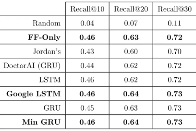
For Mimic-III, the average results, presented in Table 3, demonstrate superior performance, with up to 73% accuracy for Recall@30, for techniques Google-LSTM and Minimal GRU. Unexpectedly,
405
the feed-forward-only network had a performance comparable to classic LSTM and GRU, with up to 72% accuracy for Recall@30. The probable reason is that more than 68% of the patients with more than one admission have only two admissions – actually, only roughly 32% of these patients have between three and four admissions. That is, Mimic-III sets circumstances in which the time-awareness or recurrent cells is not necessary for a great part of its data.
410
To confirm our results, the same experiments ran over dataset InCor. Only the techniques with best performances were considered as seen in Table 3 – that is, all but Random and Jordan’s. According to the results presented in Table 4, since InCor uses as much as 3,133 diagnosis codes, the performance was overall worse than that obtained over Mimic-III. Still, according to Table 4, Google-LSTM and MinGRU performed well again, but the FF-Only network failed remarkably.
415
Concerning FF-Only, we verified that, while Mimic-III has nearly 32% of the patients with less than four admissions, in InCor, nearly 55% of the patients have between three and eleven admissions; that is, for InCor, the time-awareness of recurrent cells is much more essential.
We verified that DoctorAI (GRU+embedding) and cell GRU itself had the best performances for InCor, although the difference was not pronounced. For all the aforementioned results, neuron
420
cells GRU, MinGru, and Google-LSTM were kept for the next round of experiments.
6.4.2. Experimenting with the number of layers and neuron cells
This section relates to Section 5.2. After choosing the most adequate neuron cells, we proceeded
425
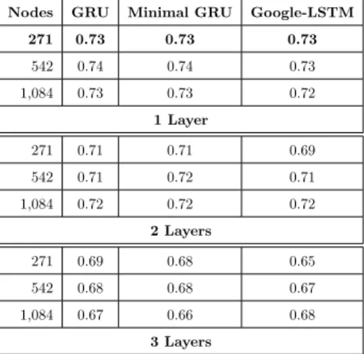
with tests regarding the number of layers and neurons. Over Mimic-III, we experimented with up to 3 layers and with 271, 542, and 1,084 cells per layer, in a total of 9 settings for cells GRU, MinGru, and Google-LSTM – the number of cells is a multiple of the size of the input layer. In Table 5, one can see that more layers caused the system to lose performance - meanwhile, the number of
Recall@10 Recall@20 Recall@30 Random 0.04 0.07 0.11 FF-Only 0.46 0.63 0.72 Jordan’s 0.43 0.60 0.70 DoctorAI (GRU) 0.44 0.62 0.72 LSTM 0.46 0.62 0.72 Google LSTM 0.46 0.64 0.73 GRU 0.45 0.63 0.73 Min GRU 0.46 0.64 0.73
Table 3: Direct comparison of eight types of artificial neuron cells using metric Recall@k for k ∈ {10, 20, 30} over dataset Mimic-III with CCS encoding. Average values computed after three runs on three different randomized splits.
Recall@10 Recall@20 Recall@30 FF-Only 0.30 0.39 0.46 DoctorAI (GRU) 0.36 0.47 0.55 LSTM 0.34 0.44 0.50 Google LSTM 0.35 0.46 0.52 GRU 0.36 0.47 0.54 Min GRU 0.35 0.46 0.53
Table 4: Direct comparison of six types of artificial neuron cells, now over dataset InCor using ICD-10, using metric Recall@k for k ∈ {10, 20, 30}. Average values computed after three runs on three different randomized splits.
neurons did not affect the results so much, but, of course, it demanded more processing time.
430
Similarly to the experiment carried out in Section 6.4.1, GRU, MinGru, and Google-LSTM had similar performances – for Mimic-III, their Recall@30 ranged from 73% to nearly 66%. In fact, their performances are virtually identical, so that any of the three neuron cells would work the same in terms of prediction performance. Concerning processing cost, the time for training three layers each with 1,084 nodes was computed. Table 6 demonstrates that Minimal GRU has the
435
smallest processing cost, finishing 55% earlier than Google-LSTM for Mimic-III and 54% for InCor; and 23% earlier than GRU for Mimic-III and 17% for InCor. These results are proportional to the number of gates of each technique and, consequently, to the number of parameters to be adjusted during training.
To double-check our conclusions, similar experiments were performed over dataset InCor;
tionally, Minimal Gated Recurrent Units are used in bidirectional parallelism. The use of dataset InCor was to guarantee that our conclusions on cardinality did not arise from specific traits found in Mimic-III. Accordingly, we experimented with up to 3 layers and with 391, 783, 1,566, and 3,133 cells per layer in a total of 12 settings. Table 7 presents the results for Recall@30. The results over dataset InCor confirmed the conclusions previously drawn with Mimic-III; that is, the more hidden
445
layers the worse was the performance for every layer size. Regarding the number of neurons per layer, one can see that bigger layers also tend to slightly reduce the performance, as well as a layer size smaller than 783, or 25% of the input size.
In conclusion, we decided for Minimal GRU as the neuron cell of our architecture, and for one single hidden layer – this architecture demonstrated better performance in terms of
predic-450
tion and processing cost. For Mimic-III, this layer should have 271 nodes, and for InCor, 783 nodes.
Nodes GRU Minimal GRU Google-LSTM 271 0.73 0.73 0.73 542 0.74 0.74 0.73 1,084 0.73 0.73 0.72 1 Layer 271 0.71 0.71 0.69 542 0.71 0.72 0.71 1,084 0.72 0.72 0.72 2 Layers 271 0.69 0.68 0.65 542 0.68 0.68 0.67 1,084 0.67 0.66 0.68 3 Layers
Table 5: Performance comparison of neuron networks GRU, Minimal GRU, and Google-LSTM with the number of layers ranging from 1 to 3, each with 271, 542, or 1,084 nodes – tests ran over Mimic-III with CCS encoding. Best performances for one single layer with 271 nodes.
Dataset/Cell GRU Minimal GRU Google-LSTM
Mimic-III 243 s 196 s 436 s
InCor 1586 s 1,318 s 2,027 s
Table 6: Training time comparison, in seconds, of neuron networks GRU, Minimal GRU, and Google-LSTM with 3 layers and 1,084 nodes per layer.
LIG-Doctor #layers/#cells 391 783 1,566 3,133
1-layer 0.70 0.72 0.70 0.69 2-layers 0.68 0.69 0.69 0.62 3-layers 0.60 0.61 0.62 0.58
Table 7: Performance comparison of different architecture sizes for LIG-Doctor’s Minimal Gated Recurrent Units organized in bidirectional parallelism over dataset InCor using ICD-10. Total of 12 different settings with 1, 2, or 3 layers, and 391, 783, 1,566, or 3,133 cells per layer. The best performance comes with one single layer with 783 nodes.
6.4.3. Further design improvements
This section relates to Section 5.3. After deciding for the Minimal GRU cell, and for the
cardinality of layers and neurons, the next step was to use more elaborated techniques to further
455
improve the performance.
We experimented with the principle of bidirectional recurrent neural networks, which led us to the parallel architecture discussed in Section 5. Over this architecture, we further experimented with other techniques, including the use of an embedding layer before the hidden layers; and the use of extra features like duration of admission, the interval between admissions, and type of the
460
admission.
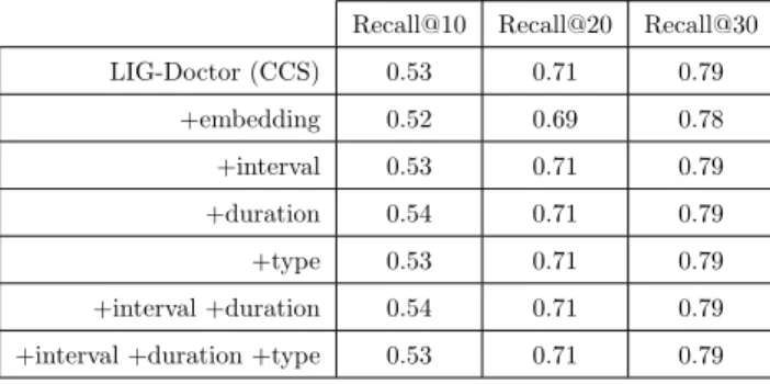
Table 8 presents results for Mimic-III. The first thing to observe is that the complete architecture yielded results significantly superior to the configurations that do not use bidirectional parallelism, as presented in Table 3. For InCor, the same fact appears when comparing Tables 10 and 4; for InCor, the results were even more pronounced since the dataset has longer temporal sequences, as
465
already pointed out in Section 6.4.1.
Still in Table Table 8, one can see that the embedding layer just reduced the performance; a side effect that we verified for all the settings previously reported. The use of embedding just added an extra layer and the behavior of the network was just the same as that observed in SubSection 6.4.2; the more layers, the worse the performance. The use of extra features found in the database,
470
namely the type of the admission (newborn, elective, emergency, or urgent), the interval between admissions, and the duration of the admissions, provided slight improvements – refer to lines 3 to 7 in Table 8. These extra features are employed via concatenation to the input tensor, without an embedding layer – the type in the form of a 4-codes hot-vector; the time in the form of a single
normalized extra slice. The first of these features, type, is very particular to Mimic-III; the interval,
475
however, applies to any other medical dataset. The final highest Recall, achieved with duration, ranged from 54% at k = 10 to 79% at k = 30, not significantly better if compared to the simplest form of the architecture presented in the first line of the table.
Recall@10 Recall@20 Recall@30 LIG-Doctor (CCS) 0.53 0.71 0.79 +embedding 0.52 0.69 0.78 +interval 0.53 0.71 0.79 +duration 0.54 0.71 0.79 +type 0.53 0.71 0.79 +interval +duration 0.54 0.71 0.79 +interval +duration +type 0.53 0.71 0.79
Table 8: Performance of our methodology over dataset Mimic-III using 271 CCS codes when combined with fur-ther techniques and data features. The best results came with the use of the duration of the hospital admission concatenated to the input data (no embedding layer); however, the improvement was not significant.
In Table 9, experiments similar to those reported in Table 8 were perform, but now using Mimic-III encoded with the entire range of 855 ICD-9 codes. The results stress the previous results; the
480
basic architecture presents the best performance, while architectural variations did not significantly improve the prediction of future diagnoses. The table also demonstrates that the use of the less granular CCS encoding, instead of ICD-9, remarkably improved the results.
Recall@10 Recall@20 Recall@30 LIG-Doctor (ICD-9) 0.48 0.64 0.72
+embedding 0.47 0.63 0.71 +interval 0.47 0.64 0.72 +duration 0.47 0.63 0.71 +type 0.48 0.64 0.72
Table 9: Performance of our methodology over dataset Mimic-III considering the entire range of 855 ICD-9 codes, instead of the 271 CCS codes. With respect to the variation of the architecture, the results were similar to the ones presented in Table 8; but with respect to the dataset encoding, the wider range of ICD-9 resulted in inferior performance.
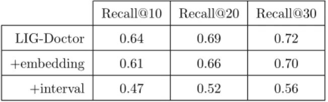
We repeated the experiments over the InCor dataset considering the basic architecture, the use of embedding, and the use of interval. The other features that tested with Mimic-III are not
available in InCor – see Table 10. Again, the use of embedding (from cardinality 3,311 to 783) did not help, resulting in nearly 5% less Recall performance. The use of interval, different from Mimic-III, was not useful either; its use resulted in a strong decrease in performance, around 20% inferior.
Recall@10 Recall@20 Recall@30
LIG-Doctor 0.64 0.69 0.72
+embedding 0.61 0.66 0.70
+interval 0.47 0.52 0.56
Table 10: Performance of our methodology over dataset InCor using ICD-10 when combined with embedding, and interval between admissions. The simplest form of the architecture presented the best results.
7. Discussion
490
Section 6.3 demonstrated that the proposed architecture presented performance superior to works from the state of the art. The results presented in Section 6.4 justified the decisions that led to the architecture described in Section 5. Furthermore, here, we discuss the interpretability and applicability of our work in Section 7.1, and insights regarding the design of artificial neural networks in Section 7.2.
495
7.1. Interpretation of results
As defined in the problem statement in Section 4, LIG-Doctor works by predicting the possible future diagnoses of a patient based on the diagnoses of this patient during former admissions. The prediction is provided in the form of probabilities p(d|x), that is, the probability of diagnosis d given the set of previous admissions x. Table 11 illustrates actual examples extracted from dataset
Mimic-500
III. We report diagnoses that the system accurately anticipated, but notice that other diagnoses are suggested each one with a probability score – these other diagnoses are also useful to the physician because they have the potential to alert for situations that occurred to other patients in similar conditions, but that did not settle yet. As reported in our previous experiments, from the top 10 recommendations with highest probabilities, on average, more than 5 of then are correct.
505
The predictions provided by techniques like LIG-Doctor and related works are meant to assist physicians in the interpretation of a patient’s EHR. Given a patient with dozens of previous ad-missions, the system will suggest to the physician a set of possible outcomes that might arise in
Previous diagnoses Predicted diagnoses
Patient 1
Coronary atherosclerosis Diabetes mellitus Chronic kidney disease
Cardiac dysrhythmias Anemia
Disorders of lipid metabolism
Patient 2
Genitourinary congenital anomalies Essential hypertension
Heart valve disorders
Fluid and electrolyte disorders Acute and unspecified renal failure
Upper respiratory disease
Patient 3
Pleurisy; pneumothorax; pulmonary collapse Cardiomyopathy
Coagulation and hemorrhagic disorders
Diseases of veins and lymphatics Disorders of stomach and duodenum
Liver diseases
Table 11: Example of real-world predictions carried out from dataset Mimic-III using the simplified CCS encoding.
the future of this patient. The benefits include faster interpretation of long medical records; em-phasis on the set of more probable outcomes reminding the physician of a broad set of situations;
510
presentation of knowledge acquired from cases related to other patients from the entire dataset, complementing the experience of the physician; opportunity for preventive medicine, since the pre-diction is, essentially, an anticipation of what might happen to a given patient; proposition of new relationships between diseases and symptoms; among other uses still to come.
7.2. On the design of neural networks
515
Our experiments also provided interesting insights. We verified that recurrent neural networks do not sustain performance as more layers are stacked – contrary to the intuition that deeper networks should work better. We also found that recurrent neural cells LSTM and GRU had performances similar to that of Minimal GRU; which, in contrast, uses a minimal number of gates. That is, a smaller number of gates per neural cell achieved performance comparable to classical,
520
more complex and costly, neural cells. Lastly, it was verified that the simplest design of one single hidden layer, structured with the simplest neural cell, provided the best results; in addition, the use of a parallel network in bidirectional fashion, instead of stacked, provided the most significant performance improvement.
Specifically concerning the open-access Mimic-III dataset, it was verified that, although it
sup-525
ports the training of recurrent neural networks for trajectory prediction, it demands the use of a less granular encoding of diagnoses due to its low cardinality; the HCUP-CCS is used in this task. Moreover, we noticed that the entire scope of ICD-9 is too broad for effective statistical and
ana-lytical tasks in general (newer ICD-10 is over four times more granular). For Mimic-III, it was also noticed that the majority of its Electronic Health Records carries sequences with only two hospital
530
temporal admissions; in this circumstance, the benefit of using recurrent neurons is minimal – as a consequence, for Mimic-III, the use of a simple feed-forward network provided reasonable results. This effect did not hold for dataset InCor, which comprises longer temporal sequences.
8. Conclusions
We worked on the design of an artificial neural network able to perform effectively in the task
535
of patient trajectory prediction. Extensive tests were performed to determine the most appropriate configuration in terms of which cell to use, which architecture, and hyper-parameters. Experiments were conducted over the open-access dataset Mimic-III, and over the private dataset InCor, both of them in the order of dozens of thousands of patient admissions; these data are used to explore several dimensions of the design space of artificial neural networks using the low-level Deep Learning
540
framework Theano. Besides leading us to the best performance, all the design process revealed relevant facts that might contribute to future works on similar problems.
As of last remarks, we mention future research. The parallel architecture demonstrated effec-tively; this design might extrapolate to more than two parallel networks, each one benefiting from different characteristics of the data – actually, most medical datasets count on semantic features
545
adequate for further investigation. It is worthy to explore specific-disease datasets as to predict finer onsets, like heart failures or strokes; even further, the use of temporal data can extrapolate to the prediction of when a certain outcome is to occur. Finally, data augmentation in the medical domain is quite desirable due to the restricted access common to most datasets; this can be accomplished with adversarial networks, which is currently an active research field.
550
Acknowledgments
This research was financed by Brazilian agencies Fundacao de Amparo a Pesquisa do Estado de Sao Paulo (Fapesp, 2018/17620-5, 2017/08376-0, and 2016/17078-0); Coordenacao de Aperfe-icoamento de Pessoal de Nivel Superior (CAPES, Finance Code 001); and Conselho Nacional de Desenvolvimento Cientifico e Tecnologico (CNPq, 406550/2018-2, and 305580/2017-5). We also
555
thank Nvidia Corporation for donating the GPUs that supported this work. This research was ap-proved by InCor’s Institutional Review Board (IRB) under number CAEE 17146019.0.0000.0068.
References
[1] Abrahao, M. T. F., Nobre, M. R. C., and Gutierrez, M. A. (2017). A method for cohort selection of cardiovascular disease records from an electronic health record system. International Journal of Medical Informatics, 102:138 –
560
149.
[2] Arandjelovic, O. (2015). Discovering hospital admission patterns using models learnt from electronic hospital records. Bioinformatics, 31(24):3970–3976.
[3] Bergstra, J. and Bengio, Y. (2012). Random search for hyper-parameter optimization. J. Mach. Learn. Res., 13:281–305.
565
[4] Bergstra, J., Breuleux, O., Bastien, F., Lamblin, P., Pascanu, R., Desjardins, G., Turian, J., Warde-Farley, D., and Bengio, Y. (2010). Theano: a cpu and gpu math expression compiler. In Proceedings of the Python for scientific computing conference (SciPy), volume 4, pages 1–7. Austin, TX.
[5] Cho, K., van Merrienboer, B., Bahdanau, D., and Bengio, Y. (2014). On the properties of neural machine translation: Encoder-decoder approaches. In Proceedings of the Eighth Workshop on Syntax, Semantics and
570
Structure in Statistical Translation, pages 103–111.
[6] Choi, E., Bahadori, M. T., Schuetz, A., Stewart, W. F., and Sun, J. (2016). Doctor ai: Predicting clinical events via recurrent neural networks. JMLR Workshop Conf Proc, 56:301–318. 28286600[pmid].
[7] Choi, E., Du, N., Chen, R., Song, L., and Sun, J. (2015). Constructing disease network and temporal progression model via context-sensitive hawkes process. In Proceedings of the 2015 IEEE International Conference on Data
575
Mining (ICDM), ICDM ’15, pages 721–726, Washington, DC, USA. IEEE Computer Society.
[8] Cost, H. and Project, U. (2015). Clinical classifications software. Technical report, Agency for Healthcare Research and Quality.
[9] Douglas Miller, D. and W. Brown, E. (2017). Artificial intelligence in medical practice: The question to the answer? The American Journal of Medicine, 131:129–133.
580
[10] Frankle, J. and Carbin, M. (2018). The lottery ticket hypothesis: Training pruned neural networks. CoRR, abs/1803.03635.
[11] Furuie, S. S., Rebelo, M. S., Moreno, R. A., Santos, M., Bertozzo, N., Motta, G. H., Pires, F. A., and Gutierrez, M. A. (2007). Managing medical images and clinical information: Incor’s experience. Trans. Info. Tech. Biomed., 11(1):17–24.
585
[12] Ghassemi, M. M., Richter, S. E., Eche, I. M., Chen, T. W., Danziger, J., and Celi, L. A. (2014). A data-driven approach to optimized medication dosing: a focus on heparin. Intensive Care Med, 40(9):1332–1339. 25091788[pmid].
[13] Glorot, X. and Bengio, Y. (2010). Understanding the difficulty of training deep feedforward neural networks. In Teh, Y. W. and Titterington, M., editors, Proceedings of the Thirteenth International Conference on Artificial
590
Intelligence and Statistics, volume 9 of Proceedings of Machine Learning Research, pages 249–256, Chia Laguna Resort, Sardinia, Italy. PMLR.
[14] Goodfellow, I., Bengio, Y., and Courville, A. (2016). Deep Learning. MIT Press. http://www.deeplearningbook. org.
[15] Hochreiter, S. and Schmidhuber, J. (1997a). Long short-term memory. Neural Computation, 9(8):1735–1780.
[16] Hochreiter, S. and Schmidhuber, J. (1997b). Long short-term memory. Neural computation, 9:1735–80. [17] Hripcsak, G., Duke, J. D., Shah, N. H., Reich, C. G., Huser, V., Schuemie, M. J., Suchard, M. A., Park, R. W.,
Wong, I. C. K., Rijnbeek, P. R., van der Lei, J., Pratt, N., Noren, G. N., Li, Y.-C., Stang, P. E., Madigan, D., and Ryan, P. B. (2015). Observational health data sciences and informatics (ohdsi): Opportunities for observational researchers. Studies in health technology and informatics, 216:574–578.
600
[18] Jensen, A. B., Moseley, P. L., Oprea, T. I., Ellesøe, S. G., Eriksson, R., Schmock, H., Jensen, P. B., Jensen, L. J., and Brunak, S. (2014). Temporal disease trajectories condensed from population-wide registry data covering 6.2 million patients. Nature Communications, 5:4022 EP –. Article.
[19] Johnson, A. E. W., Pollard, T. J., Shen, L., Lehman, L.-w. H., Feng, M., Ghassemi, M., Moody, B., Szolovits, P., Anthony Celi, L., and Mark, R. G. (2016). Mimic-iii, a freely accessible critical care database. Scientific Data,
605
3:160035 EP –. Data Descriptor.
[20] Jordan, M. I. (1997). Chapter 25 - serial order: A parallel distributed processing approach. In Donahoe, J. W. and Dorsel, V. P., editors, Neural-Network Models of Cognition, volume 121 of Advances in Psychology, pages 471 – 495. North-Holland.
[21] Linderman, S. W. and Adams, R. P. (2014). Discovering latent network structure in point process data. In
610
Proceedings of the 31st International Conference on International Conference on Machine Learning - Volume 32, ICML’14, pages II–1413–II–1421.
[22] Pascanu, R., Gulcehre, C., Cho, K., and Bengio, Y. (2014). How to construct deep recurrent neural networks. In Proceedings of the Second International Conference on Learning Representations (ICLR 2014).
[23] Pham, T., Tran, T., Phung, D., and Venkatesh, S. (2017). Predicting healthcare trajectories from medical
615
records: A deep learning approach. Journal of Biomedical Informatics, 69:218 – 229.
[24] Pirracchio, R., Petersen, M. L., Carone, M., Rigon, M. R., Chevret, S., and van der Laan, M. J. (2015). Mortality prediction in intensive care units with the super icu learner algorithm (sicula): a population-based study. The Lancet Respiratory Medicine, 3(1):42–52.
[25] Rajkomar, A., Oren, E., Chen, K., Dai, A. M., Hajaj, N., Hardt, M., Liu, P. J., Liu, X., Marcus, J., Sun, M.,
620
Sundberg, P., Yee, H., Zhang, K., Zhang, Y., Flores, G., Duggan, G. E., Irvine, J., Le, Q., Litsch, K., Mossin, A., Tansuwan, J., Wang, D., Wexler, J., Wilson, J., Ludwig, D., Volchenboum, S. L., Chou, K., Pearson, M., Madabushi, S., Shah, N. H., Butte, A. J., Howell, M. D., Cui, C., Corrado, G. S., and Dean, J. (2018). Scalable and accurate deep learning with electronic health records. npj Digital Medicine, 1(1):18.
[26] Schuster, M. and Paliwal, K. K. (1997). Bidirectional recurrent neural networks. IEEE Transactions on Signal
625
Processing, 45(11):2673–2681.
[27] Wang, X., Sontag, D., and Wang, F. (2014). Unsupervised learning of disease progression models. In Proceedings of the 20th ACM SIGKDD International Conference on Knowledge Discovery and Data Mining, KDD ’14, pages 85–94, New York, NY, USA. ACM.
[28] Zeiler, M. D. (2012). Adadelta: An adaptive learning rate method. CoRR, abs/1212.5701.
630
[29] Zen, H., Agiomyrgiannakis, Y., Egberts, N., Henderson, F., and Szczepaniak, P. (2016). Fast, compact, and high quality lstm-rnn based statistical parametric speech synthesizers for mobile devices. In Proc. Interspeech, pages 2273–2277, San Francisco, CA, USA.
Int. J. Autom. Comput., 13(3):226–234.