HAL Id: hal-01008969
https://hal.archives-ouvertes.fr/hal-01008969
Submitted on 9 Oct 2020HAL is a multi-disciplinary open access
archive for the deposit and dissemination of sci-entific research documents, whether they are pub-lished or not. The documents may come from teaching and research institutions in France or abroad, or from public or private research centers.
L’archive ouverte pluridisciplinaire HAL, est destinée au dépôt et à la diffusion de documents scientifiques de niveau recherche, publiés ou non, émanant des établissements d’enseignement et de recherche français ou étrangers, des laboratoires publics ou privés.
Structural reliability analysis of deteriorating RC
bridges considering spatial variability
Trung-Viet Tran, Emilio Bastidas-Arteaga, Franck Schoefs, Stéphanie Bonnet,
A. J. O’Connor, Francesca Lanata
To cite this version:
Trung-Viet Tran, Emilio Bastidas-Arteaga, Franck Schoefs, Stéphanie Bonnet, A. J. O’Connor, et al.. Structural reliability analysis of deteriorating RC bridges considering spatial variability. 6th International Conference on Bridge Maintenance, Safety and Management, 2012, Stresa, Italy. �10.1201/b12352�. �hal-01008969�
1 INTRODUCCION
Reinforced concrete (RC) bridges are subjected to actions that could affect its serviceability and safety during their whole life- cycle, e.g., chloride penetra-tion, fatigue, creep, etc… (Bastidas 2010). Under these actions, a structural reliability analysis is es-sential to anticipate maintenance actions that opti-mize costs and ensure appropriate levels of servicea-bility and safety. Nowadays, there are significant advances in probabilistic modeling of these deterio-ration processes. However, the most part of studies focus the reliability analysis on a single section of the structure (Stewart M.G. et al 2008). Recent works have demonstrated that deterioration process-es and loading are highly space-variant (Bastidas et al 2010). Therefore, the consideration of their spatial variability is essential for proper reliability assess-ment.
Within this context, this paper focus to analyses reliability structural considering the spatial variabil-ity of its parameter. The firth, we proposes an exten-sion of random field theory for modeling spatial var-iability of deterioration processes and an expansion Karhunen-Loève is used (section 3). Thus, the stud-ied structure is discredited into several elements and system reliability is used to evaluate the probability of failure. Herein, we propose method estimation se-ries system reliability (section 4). Some considera-tions for optimal discretization will be also discussed in the paper. The proposed methodology will be ap-plied to the reliability analysis of a RC bridge girder placed in a chloride-contaminated environment. Data coming from real measurements will be used in both
the definition of the variables with larger spatial var-iability and in their characterization (section 5). The results of this study illustrate the importance of in-cluding spatial variability in the problem.
2 CHLORIDE-INDUCED RC DETERIORATION IN SATURATED ENVIRONMENTS
Assessment of corrosion effects on RC structures is a difficult task because several deterioration mecha-nisms interact in the process. The deterioration of RC induced by corrosion involves the interaction be-tween three mechanisms: ingress of the corroding agent –i.e., chlorides or carbon dioxide, corrosion of reinforcing steel and concrete cracking. The ingress of the corroding agent induces corrosion of the rein-forcing bars. The accumulation of corrosion products in the steel/concrete interface generates concrete cracking, which plays an important role in the steel corrosion rate when excessive concrete cracking is reached. Based on the previous considerations, the corrosion process is divided into two stages namely ‘corrosion initiation’ and ‘corrosion propagation’. The following sections describe the physical phe-nomena as well as outline the adopted models to de-termine the time to corrosion initiation caused by chloride ingress
2.1 Chloride ingress mechanism and modeling Fick's second law of diffusion is usually used to study the flow of chlorides into concrete (Tuutti, 1982); then for the unidirectional case (flow in x-direction):
Structural reliability analysis of deteriorating RC bridges considering
spatial variability
T.V. Tran, E. Bastidas-Arteaga, F. Schoefs, S. Bonnet
LUNAM Université, Université de Nantes, Institute for Research in Civil and Mechanical Engineering, CNRS UMR 6183, Nantes, France
A.J. O’Connor
Trinity College Dublin, Ireland
F. Lanata
Ecole Supérieure du Bois, Nantes, France
ABSTRACT: This paper proposes an extension of random field theory for modeling spatial variability of de-terioration processes, herein, the expansion Karhunen-Loève is used. The studied structure is discretized into several elements and system reliability is used to evaluate the probability of failure. Some considerations for optimal discretization will be also discussed in the paper. The series system methodology will be applied to the reliability analysis of a RC bridge girder placed in a chloride-contaminated environment. The results of this study illustrate the importance of including spatial variability in the problem.
² 2 x C D t C fc c fc ∂ ∂ = ∂ ∂ (1)
where Cfc is the concentration of chlorides dissolved
in the pore solution, t is the time and Dc is the
effec-tive chloride diffusion coefficient. Assuming that concrete is a homogeneous and isotropic material with the following initial conditions: (1) the concen-tration is zero at t=0 and (2) the chloride surface concentration is constant; the free chloride ion con-centration C(x, t) at depth x after time t for a semi-infinite medium is:
− = t D x erf C t x C c s 2 1 ) , ( (2)
Where Cs is chloride surface concentration and
erf() is the error function.
The closed-form solution of Fick's diffusion law can be easily used to predict the time to corrosion in-itiation. However, equation (2) is valid only when RC structures are saturated and subjected to constant concentration of chlorides on the exposed surfaces. These conditions are rarely present for real structures because concrete is a heterogeneous material that is frequently exposed to time-variant surface chloride concentrations. Besides, this solution does not con-sider chloride binding capacity, concrete aging and other environmental factors as temperature and hu-midity (Saetta et al 1993; Bastidas et al 2010, 2011). The European Union project, (Duracrete, 2000), proposes an expression similar to equation (2) which considers the influence of material properties, envi-ronment, concrete aging and concrete curing on the chloride diffusion coefficient:
− = t t t D k k k x erf C t x C D n c t e s 0 0 2 1 ) , ( (3)
where ke is an environmental factor, kt is a factor
which considers the influence of the test method to
measure the diffusion coefficient Do, kc is an
influ-ence factor for concrete curing, Do is the chloride
migration coefficient measured at defined
compac-tion, curing and environmental conditions, to is the
reference period to measure Do and nD is the age
fac-tor. The lifetime assessment resulting from this ap-proach is better than the one provided by equation (2) because it accounts for the type of concrete, the
w/c ratio, the environmental exposure (submerged,
tidal, splash and atmospheric), aging and concrete curing. In addition, the strength of the Duracrete ap-proach lies in considering the randomness related to chloride penetration. Although this method does not take into consideration chloride flow in unsaturated
conditions, this model will be used herein to illus-trate the phenomena of spatial variability of corrod-ing RC structures.
2.2 Corrosion initiation
After corrosion initiation, the diameter reduction of reinforcing bars induced by corrosion can be esti-mated in terms of a change in the volumetric rate by using Faraday’s law:
∫
− = t t corr u ini dt t i d t d () 0 0.0232 () dp(t)=d0−0.0116α∫ttiniicorr(t)dt (4)where du(t) and dp(t) are the residual diameters of the
reinforcing bar at time t for uniform and pitting
cor-rosion, respectively, d0(t) is the initial diameter of
the bar in mm, α is the ratio between pitting and
uni-form corrosion depths, and icorr(t) is the time-variant
corrosion rate (µA/cm2). Given the complexity of the
corrosion process in RC, icorr depends on many
fac-tors such as concrete pH and availability of oxygen, and water in the corrosion cell. However, for the sa-ke of simplicity, this work assumes that corrosion rate is constant after corrosion initiation.
3 PROBABILISTIC MODELING
3.1 Probability of corrosion initiation
The time to corrosion initiation, tini, is defined as the
time at which the chloride concentration at the steel
reinforcement surface reaches a threshold value, Cth.
This threshold concentration represents the chloride concentration for which the rust passive layer of steel is destroyed and the corrosion reaction begins. Note that this threshold is sensitive to the chemical characteristics of concrete components: sand, gravel
and cement. Therefore, it is assumed herein that Cth
is a random variable. The time to corrosion initiation is obtained by evaluating the time-dependent varia-tion of the chloride concentravaria-tion at the reinforcing steel. This is computed in this work by using equa-tion (3). The cumulative distribuequa-tion funcequa-tion of the
time to corrosion initiation, Ftini(t), is defined as:
∫ = ≤ = ≤t ini t ini ini t t P t t f x dx F ( ) ( ) ( ). (5)
The limit state function that defines corrosion ini-tiation can be written as:
) , ( ) ( ) , ( t C C t g X = th X − tc X (6)
where Ctc(X, t) is the total concentration of chlorides
at the concrete cover depth ct at time t. The
probabil-ity of corrosion initiation, pini, is obtained by
inte-grating the joint probability function over the failure domain –i.e., equation (5)
3.2 Probability of failure
In this section, we considered the probability of fail-ure of a structfail-ure concrete submitted by a loading S and determined by:
∫
= ≤ =P M t M t f x dx t Pf(X, ) ( R(X, ) S(X, )) ( ) (7)where X is the vector of random variables and f(x) is
the joint probability density function of X, MR and
MS is a capacity moments and effected moment of
the structure at the time t. If structural failure is achieved when the crack or pit size reaches a critical value, inducing the cross-section failure, the limit state function becomes:
(
( ),)
( ) ) ), ( (As a X MR As a X Ms X g = − (8)where As(a) is the net steel area, X is the vector of
random variables (i.e., applied load, concrete
com-pressive strength, etc.), MR(As(a), X) is the bending
moment capacity and MS(X) is the applied moment
at the time t. With the As(a) is determined by (Mark
G.S. et all 2008): ≥ ≤ ≤ − ≤ − − = 0 0 0 1 2 0 2 1 0 ) ( 0 ) ( 2 2 ) ( 4 ² ) ( d t p if d t p d if A A d t p if A A d a As π (9) where , ) ( . 2 arcsin . 2 , arcsin . 2 , )² ( )² ( . 5 . 0 , )² ( 2 2 5 . 0 , ) ( 1 ) ( . 2 . . 0016 . 0 ) ( 2 0 1 0 2 2 0 0 2 0 1 1 2 0 = = − = − − = − = = t p b d b d t p b t p A d t p d b d A d t p t p b i t p cross θ θ θ θ α (10)
with d0 is the initial diameter of the steel bar.
And the equation (7) will be replaced by:
(
)
∫
∞ − = ≤ = 0 ). ( 0 ) ), ( (A a X f x dx g P Pf s (11) 3.3 Spatial variabilityRisk Based Inspection analysis or reliability methods applied to real structures generally assume:
- Either that there is no stochastic field involved in the problem;
- Neither that the location of the most critical defect from reliability point of view is known and the dis-tribution of defects in the neighboring doesn’t affect the reliability.
It is well known that the reality is more complex and that we should account for stochastic fields too and non perfect inspections for condition assessment. Then the stochastic field could take several forms more or less complicated:
- The most simple is the stationary stochastic field that is able to model the chloride distribution or oth-er propoth-erties in the concrete for instance (Bazant 1991, 2000a, 2000b);
- More sophisticated is the piecewise stationary pro-cess that can integrate the variability of the con-creating by steps or the corrosion of structures in contiguous but different environments;
- Finally, fully non stationary fields are certainly the most acceptable for a fine representation of proper-ties.
However, except for natural soils, materials used for bridges building are produced following a quality process and control. We can consider that some vari-ation are fair, for instance the spatial change of the mean value. This paper focuses on the first case on-ly.
3.3.1 Description the spatial variability
With the hypothesis the stationary stochastic field, the spatial variability will be represented by a trajec-tory with the distance. In this paper, we used an ex-pansion Karhunen – Loève to represent the spatial variability (Schoefs et all 2011):
) ( ). ( . . ) , ( 1 x f x Z i n i i i Z Z
∑
= + =µ σ λ ξ θ θ (12)where, µZ is value mean of the field of Z, σZ is
val-ue standard deviation of the field of Z, n is number
of terms in the expansion,
ξξξξ
I is a set of centeredGaussian random variable reduced,
λ
i and fi arere-spectively the eigenvalues and eigenfunctions of the
covariance function: ρ( x∆ )
To determine the eigenvalues λi and
eigenfunc-tions fi, we assume that the field is second order
sta-tionary and use the exponential form of correlation function as follows: 0 ; exp ) ( > ∆ − = ∆ with b b x x ρ (13)
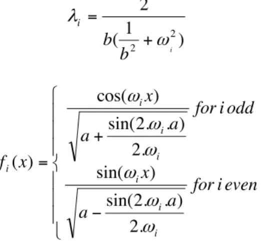
And obtain results of eigenvalues and eigenfunctions λi and fi:
) 1 ( 2 2 2 i b b i ω λ + = (14) − + = even i for a a x odd i for a a x x f i i i i i i i ω ω ω ω ω ω . 2 ) . . 2 sin( ) sin( . 2 ) . . 2 sin( ) cos( ) ( (15)
where, b is lounge of correlation and ωi is solution
of transcendental equations: = − = − even i for a b odd i for a b 0 ) . tan( 1 0 ) . tan( 1 ω ω ω ω (16)
3.3.2 Spatial variability of moment capacity. In this paper, we consider that concentration chlo-rides surface Cs and the diffusion coefficient D0 are a
stochastic field and represented by equation 12. And we obtain the cross-section area of armature by equation 3 and 9 along the RC beam.
The moment capacity of the RC beam is a func-tion of concrete compressive strength, fc’; effective
depth d; beam width, b; yield stress, fy and
cross-sectional area of armature As(a). The moment
ca-pacity can closely be approximated as:
(
)
− = b f f a A d f a A X a A M c y s y s s R . ). ( 5 . 0 ). ( ), ( ' (17)for singly reinforced rectangular beams. If the rein-forcement layout comprises n reinforcing bars then moment capacity of the beam is a parallel system di-rectly proportional to them sum of yield capacity of each reinforcing bar at time t. The moment capacity at any element j at time t is:
( )
− = b t f t f t a A d t f t a A t M cj yj sj y sj Rj ). ( ) ( ). , ( 5 . 0 ) ( ). , ( ' (18)We assume that RC beam comprising m ele-ments, parameter of each element is constant, and the failure mode of the beam will be modeled as a series system. More detailed numerical modeling will lead to more accurate estimates of structural ca-pacities of corroding structures.
4 STRUCTURAL RELIABILITY ANALYSIS CONSIDERING SPATIAL VARIABILITY OF GEOMETRICAL CHARACTERISTIC
For the series system, the critical limit state occurs when actual load effects exceed the resistance at any
element. In general, if it is assumed that n load events S at times t. With a beam comprising m ele-ments, the critical limit state at ith element is:
) , ( ) , ( ) , ( t M t S t G i i i X = R X − X (19) where MRi and Si represents the structural resistance
and load effect at the mid-point of ith element. With the n load event, we obtain Gi is a random variable.
The cumulative probability of failure of the RC beam at the time t is:
[
]
0 ) , ( ... 0 ) , ( 0 ) , ( 1 1 2 > ∩ ∩ > ∩ > − = t X G t X G t X G P P m fS (20) And[ ]
(
β, ρ)
1 m ! fS P = −Φ (21)where, Φm is a multinormale distribution, ββββ is a
vec-tor of reliability indices, β!=
{
β1,β2,...,βm}
with βiis a reliability indices of the element ith and [ρ] is a matrix correlation of the limit state G.
If it is assumed that failure elements are independ-ent elemindepend-ents, then the cumulative probability of fail-ure is:
[
]
∏
= ≤ − − ≈ m i i fS P G X t P 1 0 ) , ( ( 1 1 (22)To solution equation (21), the FORM method will be used and based on Bi-normal problem. The prin-cipal in this method, we use Bi-normal model for the replacement each of two elements by one equivalent element. Figure 1 show detail this method.
Figure 1: Description evaluation reliability structural in series system method
The firth, we will replace two elements E1 and E2
by one equivalent element E12 with value reliability
indices β12 calculated by:
[
2( 1, 2, 12)]
1
12 β β ρ
β =Φ− Φ (23)
And the correlation coefficient entre new
equiva-lent element E12 with element ith, i=3…m, ρ12k
2 12 12 12 12 * 1 * k k k B A ρ ρ β β − + = (24)
where, β12k is an equivalent reliability index of E1,
E2 and Ek :
(
2( 1 , 2 , 12 ))
1
12k β k β k ρ k
β =Φ− Φ (25)
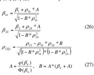
where, β1k , β2k , ρ12|k determinate by:
(
) (
2)
2 2 1 2 1 12 12 2 2 2 2 2 2 1 1 1 1 * 1 * * 1 * * * 1 * * 1 * k k k k k k k k k k k B B B B A B A ρ ρ ρ ρ ρ ρ ρ ρ β β ρ ρ β β − − − = − + = − + = (26) ) ( * , ) ( ) ( A A B A k k k + = Φ = β β β ϕ (27)where, φ(.) noted the PDF of Normal distribution standard.
The Monte-Carlo simulation is used herein to evaluate equation (19). At each element ith
at the time
t, the limit state Si is randomly generated, for this paper,
we consider the random Gaussian.
In the numerical example later, we present results for the reliability structural with the correlation between el-ements.
5 ASSESSMENT OF THE
AUTOCORRELATION PARAMETER
We assume that the stationary stochastic field can be characterized by an autocorrelation function (ACF).
Table 1 presents the most interesting ACF consid-ered for spatial variability of structures with their pa-rameter, called scale of fluctuation θ. A complete overview of the auto-correlation functions and their application is available in Kenshel (2009).
Two major procedures have been reported in the lit-erature for the estimation of θ for a spatially variable property from a digitized record of data. In the first procedure, reported by Li (2004), the Maximum Likelihood Estimate method (MLE) is used in which different values for the model parameter of the pro-posed ACF model is assumed and the value that maximizes the corresponding MLE is taken as the model parameter. In the second procedure, proposed by Vanmarke (1983), a proposed ACF model (from Table 1) can be adjusted to provide the best fit to the actual sample correlation coefficients ρ(∆x) thereby providing estimates of the corresponding model pa-rameter (i.e. a, b, c, d, e or f in Table 1).
Table 1: Autocorrelation function and corresponding scale pa-rameter θ
In this paper, we select the model 2:
0 ; exp ) ( > ∆ − = ∆ with b b x x ρ (28)
and we use the likelihood estimate for the estimation of b. − = − =
∑
∏
= = 2 exp 2 1 2 exp 2 1 1 2 1 2 k i i k k i i L ν π ν π (29)Where νi is the ith component of the vector of
inde-pendent standard values obtained from equation:
− = − Z Z z C σ µ ν 1 (30)
where z is the vector of realizations of random
vari-able Z, µz and σz respectively the mean value and the
standard deviation of the stationary field Z(x,θ) , and
C a lower triangular matrix such that CCT= ρ ρ ρ ρ and ρρρρ
the autocorrelation matrix.
And, maximize L is equivalent to minimize L1:
∑
= = k i i L 1 2 1 ν (31) The data treatment lies on a previous physical analysis to gather similar situations and distinguish others. By considering the second Fick law withoutinitial chloride concentration (i.e. C0=0) we consider
that:
-the apparent coefficient of diffusion D0 depends
on the material and the quality of concreting and is assume not to be influence by the exposure;
-the surface chloride content CS depends on the
environment and two exposures are considered: for each beam: north and south.
ACF Name ACF Model Scale of
fluctuation θ Reference 1 Triangular | | 1 , | | ( ) 0 | | for a a for a τ τ ρ τ τ − ≤ = > a (Vanmarcke, 1983) 2 Exponential ( ) exp b τ ρ τ = − 2b (Vanmarcke 1983) 3 Second-order autoregressive ( ) 1 c exp c τ τ ρ τ = + ⋅ − 4c (Vanmarcke 1983) 4 Square exponential (Gaussian) 2 | | ( ) exp d τ ρ τ = − πd (Vanmarcke 1983) 5 Cosine
exponential ( ) exp e cos e
τ τ ρ τ = − ⋅ e (Kim, 2005) 6 Sinusoidal sin 2.2 ( ) 2.2 f f τ ρ τ τ − = − f (Gomes and Awruch, 2002)
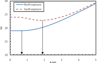
For the structure considered in section 5, Figure 2 shows the evolution of L1 with scale of fluctuation b
for Cs and two minimum values of this function are
obtained for the two exposures: 0.7 and 1.9 respec-tively for the North and the South exposures.
Figure 2: Evolution of function L1 with scale of fluctuation b of Cs (Data of Bridge Ferry-Carring, Irlande)
Figure 3 gives the same representation for the scale of fluctuation of D0. The minimum values for
the two exposures are more close 0.8 and 1.4 respec-tively for the North and the South exposures. That confirms that the scale of fluctuation should be the same because governs by the material properties and not the exposure. The value 1.1 that corresponds to the merging of data at North and South exposure is selected in the following.
Figure 3: Evolution of function L1 with scale of fluctuation b of D0 (Data of Bridge Ferry-Carring, Irlande)
6 NUMERICAL EXAMPLE 6.1 Problem description
In this paper, we present the influence of variable spatial of the geometrical characteristics Cs and D0
in the reliability analyses of RC beam (Figure 4). We consider here three materials:
- Poor: cover =38mm, w/c=0.65 and f’ck=28 MPa.
- Fair: cover =38mm, w/c=0.50 and f’ck=40 MPa.
- Good: cover =38mm, w/c=0.45 and f’ck=46
MPa.
With two conditions different of environment: Tidal and Atmospheric. The considered random variables are presented in Table 2.
Figure 4: Configuration of the bridge girder
Table 2: Statistical and deterministic parameters for the consid-ered variables of the RC beam
Variable Distribution Mean COV P Lognormal 115kN 0.20
fc’ Poor Normal 37MPa 0.15 Fair Normal 53MPa 0.15 Good Normal 61MPa 0.15
fy Normal 600MPa 0.10 ke Deterministic 0.924
kt Deterministic 1 kc Deterministic 0.8
D0 Poor Normal 1320mm²/yr 0.07 Fair Normal 473mm²/yr 0.09 Good Normal 316mm²/yr 0.10
t0 Deterministic 28 days Ccr Poor Normal 0.675* 0.27 Fair Normal 0.900* 0.17 Good Normal 0.875* 0.16 ACs** Tidal Normal 7.758 0.17 Atmospheric Normal 2.565 0.14 εCs** Tidal Normal 0 σ=1.105 Atmospheric Normal 0 σ=0.405 nD Determined 0.4 α Gumbel 5.56 0.22
icross Normal 2 µA/cm² 0.10 * Percentage of weight of binder; ** to estimate Cs=ACs(w/c)+εCs
6.2 Results
In the firth results, this paper presents the influence of spatial variability in probability of corrosion initi-ation. In Figure 5 present the probability with the three cases of type material without spatial variabil-ity. It shows that influence of corrosion in structure is different when the environment is variable. We re-alize also that, with the same material, if structure put in Tidal environment, the corrosion is faster than
Live load, P Dead load
in the Atmospheric. The influence of environment into corrosion is clear than type material. In all re-sults later, we focus calculate the Tidal environment.
Figure 5: The cumulative distribution function of the time to corrosion initiation
Figure 6 and Figure 7 show the influence of spatial
variability in the probability of corrosion initiation. With the considering the spatial variability and the correlation between elements, we realize that at the time t, when considering this variability, structure reaches its limit state faster than without the consid-ering (you see in Figure 6, this factor can reach to 200%). So, the considering in estimate reliability structure is indispensable. In results later, we will detail this influence in estimation of reliability struc-ture of RC beam.
Figure 6: Influence of spatial variability in the probability of corrosion initiation (the case Fair in Tidal environment)
Figure 7: Influence of spatial variability in the probability of corrosion initiation (the case Good in Tidal environment)
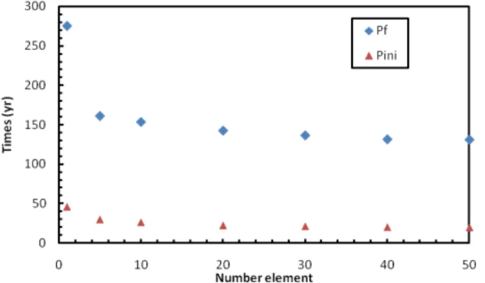
Figure 8 and Figure 9 presents the results of prob-ability of failure in the case with and without consid-ering the spatial variability of the case study of Tidal environment. Based on the results, we can also real-ize that probability of failure obtained by consider-ing spatial variability are higher than for the case without spatial variability.
Figure 8: Influence of spatial variability in the probability of failure (the case fair in Tidal environment)
Figure 9: Influence of spatial variability in the probability of failure (the case Good in Tidal environment)
If we give a critical of probability of failure, we will obtain the result that show influence of spatial varia-bility into the time initiation corrosion and the time reinforcement of structure. In the result later (Figure 10 and Figure 11), we present for example: Pf =0.5.
Figure 10: Estimation the times reinforced the RC beam (the case Fair in Tidal environment)
Figure 11: Estimation the times reinforced the RC beam (the case Good in Tidal environment)
It can be noted that with a critical accepted of probability of failure, the times reinforced of RC beam obtained by the considering spatial variability is smaller than for the case without the variable from 10 to 50%.
7 CONCLUSIONS
This paper presented the model assessment prob-ability of failure in considering spatial variprob-ability of RC beam. The method based on problem Binormale and FORM method in calculated the multi-distribution integral. The results of the numerical ex-ample show that influence of spatial variability is very important in assessment reliability structural. The considering of spatial variability of corrosion in estimation probability of failure is indispensable. The results show that the failure probabilities within spatial variability are higher than without the varia-ble from 10 to 50%.
8 ACKNOWLEDGEMENTS
The authors would like to thank the ECND-PdL pro-ject (propro-ject about Condition Assessment, Monitor-ing and Non Destructive in the Pays de la Loire re-gion) to support this project. Contact: [email protected].
9 REFERENCES
Bastidas-Arteaga E, Chateauneuf A, Sánchez-Silva M, Bresso-lette Ph, Schoefs F. 2010. Influence of weather and global warming in chloride ingress into concrete: a stochastic ap-proach.Structural Safety, 32:238-249
Bastidas-Arteaga E, 2010. Probabilistic service life model of RC structures subjected to the combined effect of chlorides-induced corrosion and cycle loading. PhD thesis. University of Nantes, France.
Bastidas-Arteaga E, Chateauneuf A, Sánchez-Silva M, Bresso-lette Ph, Schoefs F, 2011. A comprehensive probabilistic
model of chloride ingress in unsaturated concrete.
Engi-neering Structures, 33:720-30
Bazant Z. P., Novák D. 2000a. Probabilistic Nonlocal Theory for Quasibrittle Fracture Initiation and Size Effect. I: Theo-ry. Journal of Engineering Mechanics. Vol. 126, No. 2, 166-174..
Bazant Z. P., Novák D. 2000b. Probabilistic Nonlocal Theory for Quasibrittle Fracture Initiation and Size Effect. II: Ap-plication. Journal of Engineering Mechanics. Vol. 126, No. 2, 175-185.
Bazant Z. P., Xi Y. 1991. Statistical Size Effect in Quasi-brittle Structures: II. Nonlocal Theory. ASCE J. of Engrg. Mech. Vol. 117, No. 11, 2623-2640.
Duracrete 2000. Statistical quantification of the variables in the limite state functions. Technical report, The European Un-ion – Brite EuRam III – Contract BRPR-CT95-0132- Pro-ject BE95-1347/R9.
Gomes, H. M., and Awruch, A. M. 2002. Reliability of rein-forced concrete structures using stochastic finite elements.
Engineering Computations, 19(7-8), 764- 786.
Kenshel O.M 2009. Influence of spatial variability on whole life management of reinforced concrete. PhD Thesis, Uni-versity of Dublin, Trinity College, August 2009.
Li, Y. 2004. Effect of spatial variability on maintenance and repair decisions for concrete structures. PhD thesis, Delft University, Delft, Netherlands.
Saetta, A., Scotta, R., and Vitaliani, R. 1993. Analysis of chlo-ride diffusion into partially saturated concerte. ACI
Materi-als Journal, 90(5):441-451.
Schoefs F, Tran TV, Bastidas-Arteaga E. Optimization of in-spection and monitoring of structures in case of spatial fields of deterioration/properties. In: 11th International Conference on Applications of Statistics and Probability in Civil Engineering, ICAPS 11, Zurich, Switzerland; 2011. p. 2249-2256.
Stewart M.G., and Al-Harthy A. 2008. Pitting corrosion and structural reliability of corroding RC structures: Experi-mental data and probabilistic analysis. Reliability
Engineer-ing and System Safety, 93, 373-382.
Tuutti, K. 1982. Corrosion of steel in concrete. Swedish Ce-ments and Concrete Institute.
Vanmarcke, E. 1983. Random fields: analysis and synthesis,
MIT Press, Cambridge, Mass; London.
Vanmarcke, E. and Grigoriu, M. 1983. Stochastic Finite Ele-ment Analysis of Simple Beams. Journal of Engineering
Mechanics, 109(5), 1203-1214.
Yuan X.-X. and Pandey M.D. 2006. Analysis of approxima-tions for multinormale integration in system reliability com-putation. Structural Safety, 28, 361-377.
View publication stats View publication stats