HAL Id: hal-01795885
https://hal.archives-ouvertes.fr/hal-01795885
Submitted on 18 May 2018
HAL is a multi-disciplinary open access
archive for the deposit and dissemination of
sci-entific research documents, whether they are
pub-lished or not. The documents may come from
teaching and research institutions in France or
abroad, or from public or private research centers.
L’archive ouverte pluridisciplinaire HAL, est
destinée au dépôt et à la diffusion de documents
scientifiques de niveau recherche, publiés ou non,
émanant des établissements d’enseignement et de
recherche français ou étrangers, des laboratoires
publics ou privés.
Structure of the hydraulic jump in convergent radial
flows
Kseniya Ivanova, S. Gavrilyuk
To cite this version:
Kseniya Ivanova, S. Gavrilyuk. Structure of the hydraulic jump in convergent radial flows. Journal of
Fluid Mechanics, Cambridge University Press (CUP), 2019, 860 (pp. 441-464). �hal-01795885�
Structure of the hydraulic jump in convergent radial flows
K.A. Ivanova
∗, S.L. Gavrilyuk
†,
May 18, 2018
Abstract
We are interested in modelling of multi–dimensional turbulent hydraulic jumps in conver-gent radial flow. To describe the formation of intensive eddies near the free surface (rollers) at the front of the hydraulic jump, a new model of shear shallow water flows is used. The governing equations form a non–conservative hyperbolic system with dissipation source terms. The structure of equations is reminiscent of generic Reynolds-averaged Euler equations for barotropic compressible turbulent flows.
Two types of dissipative terms are studied. The first one corresponds to Ch´ezy-like
dis-sipation rate, and the second one to a standard energy disdis-sipation rate commonly used in compressible turbulence. Both of them guarantee the positive definitness of the Reynolds stress tensor. The equations are rewritten in polar coordinates and numerically solved by using an original splitting procedure. Numerical results for both types of dissipation are presented and qualitatively compared with the experimental works. The results show both experimentally observed phenomena (cusp formation at the front of the hydraulic jump) as well as new flow patterns (the shape of the hydraulic jump becomes a rotating square).
Key words: turbulent hydraulic jump, convergent radial flow, radial symmetry breaking, non-conservative hyperbolic equations
1
Introduction
Much work has been done in the study of the hydraulic jumps in a divergent radial flow [1], [2], [6], [14], [15], [16], [17], [18], [22], [25]. Such a flow can easily be created by a vertical impact of a jet of water on a solid flat surface. After the impact, the flow spreads radially outwards and at some distance of the point of impingement an abrupt depth transition occurs (hydraulic jump appears). Despite the radial symmetry of the initial flow and corresponding boundary conditions, the hydraulic jump is not necessary circular: its shape can have even polygonal structure with sharp corners (see [3, 4, 5]).
An interesting experimental study was also recently performed by [7, 8] for convergent radial flows. A radial symmetry breaking was also observed: under some flow conditions a rotating singular point (a cusp) appears at the front of the hydraulic jump.
A reliable mathematical model which is capable to capture this complex phenomenon of sym-metry breaking is still lacking. The aim of this article is to model such a phenomenon by using the model of shear shallow water flows [20, 21, 24]. Shear effects are necessary to describe surface rollers of the hydraulic jump. In 1D–case, such a model complemented by friction terms was used for the study of travelling waves down inclined plane (roll waves) and turbulent hydraulic jumps. A strong physical adequacy of the model with the experimental observations was found [13, 19, 20, 21]. The classical Saint–Venant equations were not able to describe these phenomena, because they do not take into account the vorticity effects. The new model was able to form rollers in the hydraulic jumps through the Rankine–Hugoniot relations for the corresponding hy-perbolic and conservative equations. In particular, the model was able to describe the shape of the
∗Aix Marseille Univ, CNRS, IUSTI, Marseille, France, [email protected]
1D hydraulic jump as well as oscillations of the jump toe appearing when the Froude number is larger than approximately 1.5. A natural step would be to apply this model for the description of multi–dimensional turbulent hydraulic jumps, and, in particular, to see if the model of shear shal-low water fshal-lows is able to describe the breaking of radial symmetry in hydraulic jumps observed experimentally.
The governing equations are obtained by depth averaging of multi–dimensional Euler equations [20, 21, 24]. The hypothesis of smallness of the horizontal vorticity (the hypothesis of weakly sheared flows) allows us to keep the second order depth averaged correlations in the governing equations but neglect the third order correlations, and thus to close the governing system in dissipationless limit.
The corresponding multi–dimensional model of shear shallow water flows is a hyperbolic system of equations which is reminiscent of a generic Reynolds-averaged Euler for barotropic turbulent flows. The model has three families of characteristics corresponding to the propagation of sur-face waves, shear waves and average flow. The main difficulty is non-conservativity of governing equations: for six unknowns (the fluid depth, two components of the depth averaged horizontal velocity, and three independent components of the symmetric Reynolds stress tensor) one has only five conservation laws : conservation of mass, momentum, energy and mathematical “en-tropy” . The last one determines the evolution of the determinant of the Reynolds stress tensor. The non–conservative nature of the multi-dimensional equations represents an enormous difficulty from the mathematical and numerical point of view. The definition and computation of discon-tinuous solutions for non-conservative hyperbolic equations is a challenging problem. Recently, a numerical method (a splitting procedure) was developed for solving this non-conservative system [11]. Cartesian coordinates were used for the description of multi-dimensional roll waves. In the present work we extend this technique to polar coordinates.
Another difficulty is to introduce the dissipative terms into the model. The introduction
of dissipation terms is always an empirical procedure. In particular, in [11] we proposed the dissipation terms which ensure the positive definiteness of the stress tensor P. Also, in 1D limit we recovered the dissipation law developed in [21]. In particular, this dissipation law allowed us to describe the “fingering” phenomenon (i.e. the formation of transverse waves on the front of roll waves). We will test here another type of dissipation used earlier in [12] to study the surface wave propagation in shear flows.
Different dissipation laws give us different flow patterns. The first type of dissipation give us hydraulic jumps with formation of rotating cusp at the front of the hydraulic jump as in experiments of [8]. The second type of dissipation gives us an unusual structure, which represent a smooth “square”. The square has no sharp corners and rotates with constant velocity. This is different from sharp corner structures of hydraulic jumps obtained in divergent radial flows ([4, 5]). The structure of the article is organized as follows. In Section 2 the “shear shallow water” equations are presented. Two types of dissipative terms are proposed in Section 3. Experimental works are briefly discussed in Section 4. Governing equations of sher flows rewritten in polar coordinates and the corresponding initial and boundary conditions presented in Sections 5, 6. The numerical results are discussed in Section 7. In Appendix A, the numerical scheme for the non-conservative equations is written in polar coordinates.
2
2D shear shallow water flows
The system describing multi-dimensional shear shallow water flows over a flat bottom without friction effects can be written in the form ([24, 10, 20, 21]):
∂h ∂t + div (hU) = 0, ∂ (hU) ∂t + div ( hU⊗ U + gh 2 2 I + hP ) = 0, DP Dt + ∂U ∂xP + P ( ∂U ∂x )T = 0. (1)
The system is obtained by depth averaging the Euler equations and using the hypothesis of
small-ness of the horizontal vorticity (weakly sheared flows). Here t is the time, x = (x, y)T are the
Cartesian coordinates, h is the fluid depth, g is the gravity, U = (U, V )T is the depth averaged
horizontal velocity, D/Dt means the material derivative with respect to the mean motion :
D Dt =
∂ ∂t + U
T∇, (2)
P = PT is the symmetric stress tensor which measures the distortion of the instantaneous horizon-tal velocity profile ˜U(t, x, y, z) depending of the vertical coordinate z. The definitions of U(t, x) and P are as follows:
U(t, x) = 1 h ∫ h 0 ˜ U(t, x, y, z)dz, P = 1 h ∫ h 0 ( ˜ U− U ) ⊗(U˜ − U)dz.
The tensor P is positive definite. The positive definiteness of P is a consequence of the Cauchy–
Schwarz inequality. The sign⊗ means the tensor product, I is the identity tensor. Equations (1)
admit the energy conservation law :
∂ ∂t { h ( 1 2|U| 2+ e i+ eT )} + div { hU ( 1 2|U| 2+ e i+ eT ) + ( gh2 2 I + hP ) U } = 0, (3) with ei =12(gh), eT = 12tr(P) ,
and an additional conservation law:
∂hΨ
∂t + div (hUΨ) = 0, Ψ =
Det (P)
h2 . (4)
The variable Ψ will be referred to as “entropy” (mathematical) because this quantity is transported along the mean flow in the same way as the true entropy for the Euler equations of compressible fluids. Also, we will see that this quantity will increase across the shocks in analogy with the
conventional entropy. The 1D system also admits an analogue of Ψ having a clear physical
meaning. This quantity was associated with the enstrophy (squared vorticity). For example, for hydraulic jumps the enstrophy increase corresponds to the vorticity creation : a roller appears at the forward slope of the hydraulic jump [20, 21, 13]. The system (1) is composed of the equations of mass balance, horizontal momentum and evolution equation for the stress tensor. The governing equations are hyperbolic, if P is positive definite, but not in conservative form (for proof, see [11]). For discontinuous solutions, the Rankine–Hugoniot relations come only from the mass, momentum and energy equations. For six unknowns (the fluid depth, two components of the depth averaged horizontal velocity, and three independent components of the symmetric Reynolds stress tensor) one has only five conservation laws (conservation of mass, momentum, energy and mathematical “entropy”). However, for 1D flows the system of Rankine–Hugoniot relations is closed.
3
Dissipative terms compatible with the positive
definite-ness of the Reynolds stress tensor
Now we add dissipation terms into the model. Even if this process is always empirical, some constraints should be respected. For example, the dissipation law should always be compatible with the energy decrease and guarantee the positive definiteness of the Reynolds stress tensor. Two types of dissipation terms will be tested below.
Let us add the dissipation terms in the following form : ht+ div(hU) = 0, (hU)t+ div ( hU⊗ U +gh 2 2 I + hP ) =−Cf|U|U, DP Dt + ∂U ∂xP + P ( ∂U ∂x )T = D, D = DT. (5)
In particular, the equations for P imply:
h2D Dt ( det(P) h2 ) = tr(P)tr(D)− tr(PD). (6)
The friction force in the momentum equation is a classical expression, where Cf is the Ch´ezy
coefficient. The dissipation tensor D should be somehow defined. The equations (5) should satisfy the energy conservation law :
∂ ∂t ( h ( 1 2|U| 2+ e i+ eT )) + div ( hU ( 1 2|U| 2+ e i+ eT ) + ( gh2 2 I + hP ) U ) =−Cf|U|3− Q, (7) where the dissipative source term Q should be positive. The positivity of Q is the analogue of the second law of thermodynamics. The compatibility of (5) and (7) implies the expression for Q in terms of D:
tr (D) =−2
hQ. (8)
By analogy with the Stokes hypotheses for the Navier-Stokes equations, we assume that the dissipation tensor D is an isotropic tensor function of P. Then, for two–dimensional case, D is linear in P :
D = aP + bI,
where a and b are functions of invariants of P. Consider the simplest case where b = 0. This choice allows us to obtain a natural reduction to the Saint-Venant equations in the limit P = 0.
3.1
First type of dissipation terms
The first type of dissipation is :
D = aP, a =−2αh|U|3, (9)
where a = τ−1, τ is the relaxation time, α has the dimension s2m−2. The multiplier−2|U|3/h is
for convenience only. In particular, this choice implies the equation for Ψ in the form :
h2D Dt ( det (P) h2 ) =−4α h |U| 3 det (P) . (10)
Equations (8) and (9) imply the following relation between Q and α :
We will introduce now a new dimensionless parameter κ = αtr (P). To recover the 1D case studied priviously ([20, 21]), we will finally choose :
κ = max ( 0, Cr tr(P) h2 − φ tr(P) h2 ) ≥ 0. (12)
Here φ and Cr are the model constants : φ is associated with the enstrophy of small vortexes in
the vicinity of the bottom, and Cr is the coefficient associated with the roller dissipation. We will
search the values of these parameters to have at least a qualitative agreements with experiments. As it follows from (10) and (12), “entropy” Ψ is decreasing on continuous solutions, but always stays positive. This means that the dissipation law also guarantees the positive definiteness of P.
3.2
Second type of dissipation terms
Another type of dissipation tensor D can be considered in this form:
D = aP, a =−2hκtr(P)12. (13)
As a consequence of (11), one has:
Q = κtr(P)32 > 0. (14)
This type of dissipation is Galilean invariant and was used, in particular, to study the solitary wave breaking ([12]). Moreover, (14) corresponds to the classical energy dissipation rate with the dissipation rate scale h ([26]). Such a choice also guarantees that P is positive definite for any time, if initially it was positive definite.
4
Experiments on hydraulic jumps in a radial flow
The circular hydraulic jumps are commonly observed in a kitchen sink when a vertically falling tap water jet strikes a horizontal plate and then spreads radially outwards ([1], [2], [3], [6], [15], [16], [17], [18]). Using a more viscous liquid, [3, 4, 5] observed breaking of radial symmetry of the hydraulic jump front. More exactly, [4, 5] obtained polygonal shapes of hydraulic jumps in divergent radial flow with sharp corners: “the sharp corners of the polygons carry a large radial flux, while the sides generate resistance to the stream”. [3] also noted that: “some polygonal ... forms were subject to weak time–dependent fluctuations, typically characterized by a net rotational motion of the entire jump structure, or the propagation of wave-like disturbances towards a single point on the jump”.
Our numerical study will concern the hydraulic jump in a convergent and not divergent radial flow. Such experiments were recently performed by [7, 8]. In these experiments, the fluid is radially injected inwards and strikes a hollow cylinder placed in the center, through which the water is evacuated. As a consequence, a hydraulic jump is formed separating convergent supercritical
flow from deeper subcritical one. The hydraulic jump also exhibits the appearance of radial
asymmetries: after formation of the hydraulic jump, it starts to oscillate randomly, then the amplitude of oscillations grows and, finally, the flow becomes very asymmetric and develops a singularity of the jump front that starts to rotate with a constant angular velocity.
We want to understand if model (1) is able to reproduce, at least qualitatively, the last exper-iments. Also, it would be interesting to study the influence of different types of dissipation on the solution structure and to understand if new patterns can appear.
5
Governing equations in polar coordinates
To model the hydraulic jumps in radial flow, we rewrite the system (1) in polar coordinates (see Appendix A). In dissipationless case over a flat bottom the system (1) becomes:
∂(hr) ∂t + ∂(rhUr) ∂r + ∂(hUθ) ∂θ = 0, (15)
∂(rhUr) ∂t + ∂ ∂r { r ( hUr2+gh 2 2 + hPrr )} + ∂ ∂θ(hUrUθ+ hPrθ) = h(U 2 θ + Pθθ) + gh2 2 , (16) ∂ (rhUθ) ∂t + ∂ ∂r {rh (UrUθ+ Prθ)} + ∂ ∂θ ( hUθ2+gh 2 2 + hPθθ ) =−h (UrUθ+ Prθ) , (17) DPrr Dt − 4 Uθ r Prθ+ 2 ( ∂Ur ∂r Prr+ Prθ r ∂Ur ∂θ ) = 0, (18) DPrθ Dt + Uθ r (Prr− 2Pθθ) + Pθθ r ∂Ur ∂θ + Prr ∂Uθ ∂r + Prθ r { ∂Uθ ∂θ + ∂(rUr) ∂r } = 0, (19) DPθθ Dt + 2 Uθ r Prθ+ 2 { ∂Uθ ∂r Prθ+ Pθθ r ( ∂Uθ ∂θ + Ur )} = 0, (20) ∂ ∂t { hr(12|U|2+ E)}+∂r∂ { r [ hUr (1 2|U| 2+ E)+gh2 2 Ur+ h(PrrUr+ PrθUθ) ]} + +∂θ∂ { hUθ (1 2|U| 2+ E)+gh2 2 Uθ+ h(PrθUr+ PθθUθ) } = 0, (21)
where the material derivative is defined as:
D Dt = ∂ ∂t + Ur ∂ ∂r + Uθ r ∂ ∂θ.
The system (15)–(21) admits the “entropy” conservation law:
D Dt ( det(P) h2 ) = 0. (22)
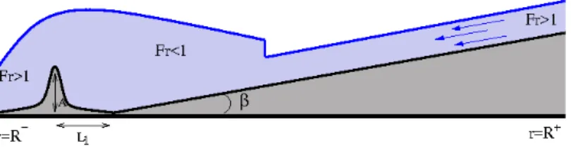
We have now to add into the model the dissipation terms and bottom topography. The bottom topography consists of an inclined plane of a mild slope superposed with a bump modeling the hollow cylinder (see Figure 1). Analytically, the expression of the bottom is given by:
b(r) = A[(r−R −−L 1)2−L21] 2 L4 1 , if 0 < r− R−< 2L1, (r− R−− 2L1) tan β, if 2L1+ R−< r < R+. (23)
Here β is a small inclination angle, A is the bump amplitude, 2L1 is the radial bump width, R−
is the internal boundary radius, R+ is the external boundary radius. The formula (23) is used to
model the “physical” cylinder of hight A which is placed at r = R−+ L1.
6
Initial and boundary conditions
Now, we need to impose boundary conditions on the cylinder. The number of boundary conditions is equal to the number of characteristics entering the flow domain. For stationary flow a natural boundary condition to impose on the top of the cylinder is the criticality condition (Froude number is equal to one). When the flow is nonstationary and transcritical, the problem of boundary conditions is an open question even for the classical Saint-Venant equations (cf. [23]). In particular, if the flow is subcrictical, the perturbations can propagate inside the domain and change the solution. We need thus a remedy to impose “good” boundary conditions. For this, we will compute the solution in a larger domain by introducing a bump, where the downslope flow accelerates and
becomes supercritical. If the flow is supercritical at both boundaries r = R− and r = R+, the
boundary conditions are simple to impose. In particular, at r = R− there is no characteristics
entering the flow domain, so we can use Neumann boundary conditions. At r = R+we impose all
unknowns. Such an approach allowing us to control the fluid flow at the downstream crest was also used by [27].
h0[m] β [rad] Cr Cf φ [s−2] q0[m3/s] R+[m] R− [m] A [m] L1[m]
0.003 0.07 0.3− 1.0 0.0036 2 − 20 1.2· 10−3 1.0 0.08 0.005 0.006
Table 1: Parameters for numerical tests.
Figure 1: The bottom topography used in numerical simulations.
We numerically solved the equations (21) where, additionally, the dissipation and bottom topography are added (see Appendix A) in the computational domain:
R−≤ r ≤ R+, 0≤ θ ≤ 2π.
The initial conditions are :
h(r, θ, t = 0) = 1.5h0[m]; if r− R−≤ 0.3(R+− R−), h0[m]; else Ur(r, θ, t = 0) =−q0/(rh), Uθ(r, θ, t = 0) = 0, Prr= φh2, Prθ= 0, Pθθ= ϵφh2.
Here ϵ = 10−8, h0 is a given flow depth at r = R+, q0> 0 is a given flow discharge. The other
parameters are shown in Table 1. Obviously, we respect the inequality 2L1< 0.3(R+− R−). We
have to underline that the initial conditions are inimportant, because for large time the solution is definied only by the boundary conditions. To avoid the degeneracy of determinant of P and ensure the hyperbolicity of the governing equations, we take a small positive value of Pθθ.
This initial radial flow is perturbed by boundary conditions at r = R+ in the following form:
h = h0, Ur=−q0(1 + 0.01 sin(nθ))/(R+h0)), Uθ= 0, Prr = Pθθ= 0.5φh20, Prθ= 0. (24)
We used here isotropic expression of P. Also, for this case one has κ = 0. We also added a small perturbation of the radial velocity in θ–direction with n being any natural number. We took
n = 16 that corresponds to the number of injecting pumps used, in particular, in experiments
by [8]. The periodic boundary condition is used in θ− direction. We control that at the inner
boundary r = R− in radial direction the corresponding generalized Froude number is larger than
one to guarantee the condition of supercritical flow : Fg=
Ur
√
gh + 3Prr
> 1.
The numerical scheme is based on the splitting technique developed in [11]. The first-order Godunov scheme with HLLC Riemann solver was used (for details, see Appendix A). The code is parallelized using the Message Passing Interface (MPI).
0.44 0.54 0.66 0.81 3.679e-01 1.000e+00 0.368 1 Time: 200.00 s 0.44 0.54 0.66 0.81 3.679e-01 1.000e+00 0.368 1 Time: 200.00 s
Figure 2: Schlieren images of the fluid depth for Saint-Venant equations are shown with quadratic
friction (F = −Cf|U|U, Cf = 0.0036, β = 0.05[rad]) on the left, and with linear friction
(F = −ν
hU, β = 0.05[rad] with kinematic viscosity ν = 10
−6[m2/s2]) on the right. The white
boundaries inside the domain correspond to strong gradients of h. Central white part corresponds
to the hole. The “schlieren” function was used in standard form: exp(−||∇h||/||∇h||max), where
|| · || means the Euclidean norm. The same “schlieren” function was used for all computations.
The first order Godunov method with HLLC Riemann solver was used with 300× 300 mesh cells.
In both cases, the hydraulic jump was stationary. The radius of hydraulic jump for the quadratic friction is a little bit larger than that for the linear friction.
7
Numerical results
7.1
Classical Saint-Venant equations
The numerical resolution of the classical shallow water equations (Saint-Venant equations) with quadratic and linear friction give us only stationary hydraulic jumps without any oscillations or formation of rotating patterns (see Figure 2). The radius of hydraulic jump for the quadratic friction is a little bit larger of that corresponding to the linear friction. The same type of discharge perturbations was used as in (24) with the same bottom topography (23).
7.2
Shear shallow water model with first type of dissipation
We present now the numerical results for the first type of dissipation given by (9). The sce-nario of the hydraulic jump formation in convergent radial flow consists of the following three different stages. First, almost radially symmetric hydraulic jump is formed at the time instant approximately 25 s (see Figure 3). One can see only small amplitude nonstationary transverse perturbations on the front of the hydraulic jump. This is clearly visible on the Figure 3 showing the distribution of Ψ = det(P)h2 . Then, the hydraulic jump is destabilized into a pattern exhibiting
sloching type oscillations at the time instant about 50 s. The oscillation period is approximately 4 seconds. In Figure 4 the schlieren images are shown at the time instants 50 s and 52 s (after the half-period of oscillations). Remarkably, in a certain domain of parameters, as the amplitude of the oscillations grows, a new free surface pattern appears. More exactly, a singular point (cusp) at the free surface of the hydraulic jump appears which starts to rotate. In Figure 5 the cusp rotating in positive direction is denoted by S. The sense of rotation can easly be understood from the Figure 5. Indeed, ahead of the cusp the front is smooth, and behind the cusp the front is rough. The sense of rotation can be changed by a small initial perturbation. If the initial condition for the
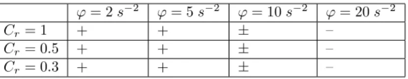
φ = 2 s−2 φ = 5 s−2 φ = 10 s−2 φ = 20 s−2
Cr= 1 + + ± –
Cr= 0.5 + + ± –
Cr= 0.3 + + ± –
Table 2: In this table, “+” means that for corresponding values of φ and Cr , the rotating cusp
is formed, “–” means that the cusp is absent.“±” means the limit behaviour.
of rotation will be determined by the sign of Uθ. The radius of the hydraulic jump increases with
time. One can also see the emergence of double jump structures appearing at time instant 150 s, where the free surface changes abruptly (Figure 5). Double jump structures were also observed in the case of divergent circular hydraulic jump in [3].
One can also notice that the cusp appears only in some region of parameters φ and Cr (see
Table 2). The existence of such a cusp allows us to easily determine the period of rotation of pattern. In particular, in our case the period of rotation was about 6 seconds. It does not depend
too much on the values of φ and Cr. In the experiments of [8] the period was was about 3 s, but
the geometry was different : the radius R+was 0.33 m. The main reason why we did not use the
same geometry was that we could not guarantee the supercritical flow at the outlet (at r = R−)
which was necessary to assure correct boundary conditions for the governing equations.
The results obtained are qualitatively similar to those observed experimentally. It means that our mathematical model of shear shallow water flows and the corresponding numerical method are capable to simulate new flow patterns appearing in radial fluid flows. The transverse structures (formation of the “triangles” behind the moving cusp) that are clearly visible in Figure 5, is a physical phenomenon and not a numerical instability. They could also be seen in the experiments of [8].
When φ vanishes, we do not obtain any transverse structures: the circular hydraulic jump is only formed. Recall, that φ is associated to the enstrophy of small vortexes at the vicinity of the bottom [20], [21].
In Table 2 we studied how parameter φ and dissipation coefficient Crinfluence the flow
behav-ior. Numerical tests showed that the more sensible parameter is φ rather than Cr. For φ larger
than 10 s−2 the cusp disappears, but the singular behaviour is still visible (see Figure 6). Numerical “cusp” solution was also obtained in [8] by using the Saint-Venant equations with linear friction, but for a different bottom topography. They used the criticality condition at the top of the cylinder what corresponds to the hypothesis of the steady flow assumption.
A surprising fact also mentioned in the experiments is that the sense of rotation of the cusp and the tangential fluid velocity near the hole is opposite. This fact is also described by our model.
7.3
Shear shallow water model with second type of dissipation
Using the second type of dissipation terms (13), one can see new unusual structures: the formation of rotating square type hydraulic jump shape (see Figure 7). The shape doesn’t contain sharp corners. In our case, the “corners” are rather smooth and the shape between “corners” is convex, while it was concave in experiments of [4]. This is the main difference between convergent and divergent radial flows. A detailed comparison of structures of divergent and convergent hydraulic jumps in shear flows will be a future work.
8
Conclusion
Numerical modeling of multi–dimensional turbulent hydraulic jumps formed in convergent radial flow is performed and qualitatively compared to the experimental observations. Two types of “well posed” dissipation terms are proposed and studied. For the first type of dissipation, in some
0.44 0.54 0.66 0.81 3.679e-01 1.000e+00 0.368 1 Time: 25.00 s -0.4 -0.2 0 0.2 0.4 -5.269e-01 5.986e-01 -0.527 0.599 Time: 25.00 s 35 70 105 140 1.408e-13 1.592e+02 1.41e-13 159 Time: 25.00 s
Figure 3: The schlieren images of h, Uθ and Ψ =
det(P)
h2 are shown. The first order Godunov
method with HLLC Riemann solver is used with 500× 500 mesh cells, Cr= 1, φ = 2 s−2. Central
white part corresponds to the hole. White line in the internal area corresponds to front of the hydraulic jump.
jump front was found. For the second type of dissipation, a smooth rotating square structure of hydraulic jump was found.
The numerical validations demonstrated the capability of the model and numerical method to reproduce the multi – dimensional hydraulic jump dynamics.
Futher development of this multi–dimensional model would be to add the dispersive effects to describe the multi-D wave propagation and breaking as was performed in 1D case in [12, 9].
Acknowledgment
The authors thank B. Nkonga, J. Massoni, S. Hank and N. Favrie for helpful discussions. This work was partially supported by l’Agence Nationale de la Recherche, France (grant numbers ANR-11-LABEX-0092, and ANR-11-IDEX-0001-02).
9
Appendix A
Governing equations in polar coordinates
We will rewrite now the system of governing equations (1) in polar coordinates. The relation between Cartesian and polar coordinates are:
x = r cos θ, y = r sin θ, r =√x2+ y2, θ = arctan(y
x
)
.
We introduce the vectors:
er= (cos θ, sin θ)T, eθ= (− sin θ, cos θ)T.
We have: ∂er ∂r = 0, ∂eθ ∂r = 0, ∂eθ ∂θ =−er, ∂er ∂θ = eθ. (25)
One can decompose:
U = Urer+ Uθeθ, ∂U ∂x = ∂U ∂r ⊗ er+ 1 r ∂U ∂θ ⊗ eθ. (26)
0.44 0.54 0.66 0.81 3.679e-01 1.000e+00 0.368 1 Time: 50.00 s -0.4 -0.2 0 0.2 0.4 -5.269e-01 5.986e-01 -0.527 0.599 Time: 50.00 s 35 70 105 140 1.408e-13 1.592e+02 1.41e-13 159 Time: 50.00 s 0.44 0.54 0.66 0.81 3.679e-01 1.000e+00 0.368 1 Time: 52.00 s -0.4 -0.2 0 0.2 0.4 -5.269e-01 5.986e-01 -0.527 0.599 Time: 52.00 s 35 70 105 140 1.408e-13 1.592e+02 1.41e-13 159 Time: 52.00 s
Figure 4: The schlieren images of h, Uθ and Ψ =
det(P)
h2 are shown. The first order Godunov
method with HLLC Riemann solver is used with 500× 500 mesh cells, Cr = 1, φ = 2 s−2. The
-0.4 -0.2 0 0.2 0.4 -5.269e-01 5.986e-01 -0.527 0.599 Time: 89.00 s 35 70 105 140 1.408e-13 1.592e+02 1.41e-13 159 Time: 89.00 s -0.4 -0.2 0 0.2 0.4 -5.269e-01 5.986e-01 -0.527 0.599 Time: 150.00 s 35 70 105 140 1.408e-13 1.592e+02 1.41e-13 159 Time: 150.00 s
Figure 5: The schlieren images of h, Uθ and Ψ =
det(P)
h2 are shown. S corresponds to a cusp
(singular point). The first order Godunov method with HLLC Riemann solver is used with 500×
500 mesh cells, Cr = 1, φ = 2 s−2. A cusp rotating in positive direction is formed. Transverse
Figure 6: Schlieren images of the hydraulic jump corresponding to φ = 2 s−2 (on the top left),
φ = 5 s−2 (on the bottom left), φ = 10 s−2 (on the top right) and φ = 20 s−2 (on the bottom
right) are shown with 500× 500 mesh cells at time instant 290 s. The value of Cr was always
taken as 0.5. The cusp is formed only for φ = 2 s−2 and φ = 5 s−2. In the case φ = 10 s−2 and
φ = 20 s−2 the cusp degenerates into a moving singular point through which we have always the transition from “smooth” to “rough” region. The corresponding singular point (denoted by S)
rotates in negative sense for all cases, excepting the case φ = 20 s−2 where the sense of rotation
is positive. The sense of rotation can easly be understood because ahead of the singular point the front is smooth, while behind the singular point the front is rough.
0.44 0.54 0.66 0.81 3.679e-01 1.000e+00 0.368 1 Time: 200.00 s -0.18 -0.12 -0.06 0 0.06 -2.093e-01 9.105e-02 -0.209 0.091 Time: 200.00 s 0.4 0.8 1.2 1.6 2 8.163e-05 2.180e+00 8.16e-05 2.18 Time: 200.00 s 0.44 0.54 0.66 0.81 3.679e-01 1.000e+00 0.368 1 Time: 196.00 s -0.18 -0.12 -0.06 0 0.06 -2.093e-01 9.105e-02 -0.209 0.091 Time: 196.00 s 0.5 1 1.5 2 2.335e-05 2.249e+00 2.33e-05 2.25 Time: 196.00 s
Figure 7: The second type of dissipation is used here. The schlieren images of h, Uθ and
Ψ = det(P)
h2 are shown at time instants 196 s and 200 s. The first order Godunov method with
HLLC Riemann solver was used with 300× 300 mesh cells, Cr= 10, φ = 100 s−2, q = 1 [L]. One
Using (25), (26), we obtain: ∂U ∂x = ∂Ur ∂r er⊗ er+ ∂Uθ ∂r eθ⊗ er+ ( 1 r ∂Ur ∂θ − Uθ r ) er⊗ eθ+ 1 r ( Ur+ ∂Uθ ∂θ ) eθ⊗ eθ. (27) (27) implies : divU = 1 r ∂Uθ ∂θ + 1 r ∂ ∂r(rUr) , (28)
Also, one has:
P = Prrer⊗ er+ Prθer⊗ eθ+ Pθreθ⊗ er+ Pθθeθ⊗ eθ, Prθ= Pθr. (29) Then, div(hP) = (div(P))h + P∇h, (30) where div(P) = ( ∂Prr ∂r + 1 r ∂Prθ ∂θ + 1 r(Prr− Pθθ), ∂Prθ ∂r + 1 r ∂Pθθ ∂θ + 2 rPrθ ) . (31) Also, DP Dt = ∂P ∂t + Ur ∂P ∂r + Uθ r ∂P ∂θ. (32)
Using (25), one obtains:
∂P ∂r = ∂Prr ∂r ∂Prθ ∂r ∂Prθ ∂r ∂Pθθ ∂r , ∂P ∂θ = ∂Prr ∂θ − 2Prθ ∂Prθ ∂θ + Prr− Pθθ ∂Prθ ∂θ + Prr− Pθθ ∂P∂θθθ + 2Prθ . (33)
One can finally obtain the system (1) in polar coordinates: ∂(hr) ∂t + ∂(rhUr) ∂r + ∂(hUθ) ∂θ = 0, ∂(rhUr) ∂t + ∂ ∂r { r ( hU2 r + gh2 2 + hPrr )} +∂θ∂ (hUrUθ+ hPrθ) = h(Uθ2+ Pθθ) +gh 2 2 , ∂(rhUθ) ∂t + ∂ ∂r{rh (UrUθ+ Prθ)} + ∂ ∂θ ( hUθ2+gh22+ hPθθ ) =−h (UrUθ+ Prθ) , ∂Prr ∂t + Ur ∂Prr ∂r + Uθ r (∂Prr ∂θ − 4Prθ ) + 2(∂Ur ∂r Prr+ Prθ r ∂Ur ∂θ ) = 0, ∂Prθ ∂t + Ur ∂Prθ ∂r + Uθ r (∂P rθ ∂θ + Prr− 2Pθθ ) +Pθθ r ∂Ur ∂θ + Prr ∂Uθ ∂r + Prθ r { ∂Uθ ∂θ + ∂(rUr) ∂r } = 0, ∂Pθθ ∂t + Ur ∂Pθθ ∂r + Uθ r (∂Pθθ ∂θ + 2Prθ ) + 2{∂Uθ ∂r Prθ+ Pθθ r (∂Uθ ∂θ + Ur )} = 0, ∂ ∂t { hr(12|U|2+ E)}+ ∂ ∂r { r [ hUr (1 2|U| 2+ E)+gh2 2 Ur+ h(PrrUr+ PrθUθ) ]} + +∂θ∂ { hUθ (1 2|U| 2+ E)+gh2 2 Uθ+ h(PrθUr+ PθθUθ) } = 0. (34) Numerical splitting technique in polar coordinates
The method follow the splitting technique proposed in [11] in Cartesian coordinates. We adapt this approach to polar coordinates. For this, we solve first the model in r-direction, then in θ-direction. For each direction, the two subsystems, proposed below, are solved separately. Each subsystem has the following properties:
• is hyperbolic
9.1
Subsystem 1 in r-direction
The first subsystem in r-direction is: ∂(rh) ∂t + ∂(rhUr) ∂r = 0, (a) ∂(rhUr) ∂t + ∂ ∂r ( r ( hU2 r + gh2 2 + hPrr )) = h(U2 θ + Pθθ) +gh 2 2 , (b) ∂(rhUθ) ∂t + ∂ ∂r(rhUrUθ) =−h (UrUθ+ Prθ) , (c) ∂(rhPrr) ∂t + ∂(rhUrPrr) ∂r + 2rhPrr ∂Ur ∂r = 4hPrθUθ, (d) ∂(rPrθ) ∂t + ∂(rUrPrθ) ∂r = Uθ(2Pθθ− Prr) , (e) ∂(hrPθθ) ∂t + ∂(rhUrPθθ) ∂r =−2h(PrθUθ+ PθθUr), (f ) (35)
The subsystem (35) admits the energy conservation law
∂ ∂t { rh ( 1 2|U| 2+ E )} + ∂ ∂r { r [ hUr ( 1 2|U| 2+ E ) +gh 2 2 Ur+ hPrrUr ]} = 0, (36) where E = (gh + Prr+ Pθθ)/2.
The system is hyperbolic with the eigenvalues given by :
λ1,2,3,4 = Ur, λ5,6= Ur±
√
gh + 3Prr. (37)
The equation (35.d) is not conservative. The jump relation for this equation is not well defined.
The value of Prr will be corrected using the energy equation (36). Numerically, we solve first the
system (35) where the equation (35.d) is replaced by
∂(rhPrr)
∂t +
∂(rhUrPrr)
∂r = 0. (38)
We update then rhPrr by using (36).
9.1.1 Godunov type method and correction of the non-conservative term rhPrr
The subsystem 1 can be rewritten in the following form:
∂W ∂t +
∂(rF)
∂r = S
r, (39)
where the vector of “conservative” variables W, the vector of fluxes F(W) and the geometric
source term vector Sr(W) here are
W =(rh, rhUr, rhUθ, rhPrr, rPrθ, rhPθθ, rh ( E +1 2|U| 2))T, F(W) =(hUr, hUr2+ p, hUrUθ, hUrPrr, UrPrθ, hUrPθθ, hUr (1 2|U| + E ) + pUr )T , (40) Sr= (0, h(Uθ2+ Pθθ ) +gh 2 2 ,−h (UrUθ+ Prθ) , 4hPrθUθ, Uθ(2Pθθ− Prr)− PrθUr, − 2h (PrθUθ+ PθθUr) , 0) with p = gh2/2 + hP rr, E = (gh + Prr+ Pθθ)/2. (41)
Let us consider now a fixed grid of size ∆r = ri+1/2− ri−1/2, the time increment is defined as
∆t = tn+1− tn that must respect the Courant-Friederichs-Lewy (CFL) condition. The discrete
values of the vector-function W at (ri, tn) will be denoted by Wni. Integrating the conservation
laws (39) on [ri−1/2, ri+1/2]×[tn, tn+1], one obtains the conservative finite volume Godunov scheme
on a fixed grid Wn+1i = Wni − ∆t ∆r ( ri+1/2(F∗,ni+1/2− S r,n i )− ri−1/2(F∗,ni−1/2− S r,n i ) ) , (42)
where F∗,ni+1/2 and F∗,ni−1/2 are the numerical fluxes. They are constant across interfaces between cells during the time step. For computing the fluxes F∗,ni+1/2 = F∗,ni+1/2(Wn
i, Wni+1) and F∗,ni−1/2 =
F∗,ni−1/2(Wn i−1, W
n
i), we use approximate solution of the Riemann problem between cells i, i + 1
and i− 1, i respectively.
Using the energy conservative law, the non-conservative term rhPrris updated by the following
way:
(rhPrr) = 2(rhE)−
g(rh)2
r − (rhPθθ). (43)
The “mathematical” entropy Ψ corresponding to the vorticity formation is increasing through the shock at this step (see for proof [11]).
9.2
Subsystem 2 in r-direction
The subsystem 2 in r-direction is: ∂(rh) ∂t = 0, (a) ∂(rhUr) ∂t = 0, (b) ∂(rhUθ) ∂t + ∂ ∂r(rhPrθ) = 0, (c) ∂(rhPrr) ∂t = 0, (d) ∂(rPrθ) ∂t + rPrr ∂Uθ ∂r = 0, (e) ∂(rhPθθ) ∂t + 2rhPrθ ∂Uθ ∂r = 0, (f ) (44)
It admits the energy conservation law :
∂ ∂t { rh ( |U|2 2 + E )} + ∂ ∂r(rhUθPrθ) = 0. (45)
The system is hyperbolic with the eigenvalues given by :
λ1,2,3,4= 0, λ5,6=±
√
Prr. (46)
Again, system (44)– (45) is overdetermined. One can note that there are two nonconservative equations. The product(rPrr∂U∂rθ
)
in equation (44.e) is well defined. It is not the case for the term (
2rhPrθ∂U∂rθ
)
in equation (44.f). In the following this equation will be replaced by ∂(rhPθθ)
∂t = 0 at
the first step, and then the energy conservation law will be used for update the value of Pθθ.
In particular, the estimation of Prθat time instant (t + ∆t) is given by:
(rPrθ) (r, t + ∆t) = (rPrθ) (r, t) + (rPrr)(r, t)
(
Uθ, i∗ −1/2(t)− Uθ, i+1/2∗ (t)
)∆t
Here Uθ∗ it is speed at the contact discontinuity. The non-conservative equation for Prθ we
dis-cretize in the following way:
Prθ(r, t + ∆t) = Prθ(r, t) + Prr(r, t)
(
Uθ, i∗ −1/2(t)− Uθ, i+1/2∗ (t)
)∆t
∆r. (48)
Here Uθ∗ is the speed of the contact discontinuity. Equation for (rhPθθ) is also non-conservative.
This equation is solved numerically first with zero flux, and then the energy conservation law was
used to update the value of rhPθθ:
(rhPθθ) = 2(rhE)−
g(rh)2
r − (rhPrr). (49)
The “mathematical” entropy Ψ is conserved at this step.
We will give now a shorter explication of splitting in θ-direction, because it is completely analogous to that in r-direction.
9.3
Subsystem 1 in θ -direction
The first subsystem in θ -direction is : ∂(rh) ∂t + ∂(hUθ) ∂θ = 0, (a) ∂(rhUr) ∂t + ∂ ∂θ(hUrUθ) = 0, (b) ∂(rhUθ) ∂t + ∂ ∂θ ( hUθ2+gh22 + hPθθ ) = 0, (c) ∂(rhPrr) ∂t + ∂(hUθPrr) ∂θ = 0, (d) ∂(rPrθ) ∂t + ∂(UθPrθ) ∂θ = 0, (e) ∂(rhPθθ) ∂t + ∂(hUθPθθ) ∂θ + 2hPθθ ∂Uθ ∂θ = 0. (f ) (50)
The subsystem (50) admits the energy conservation law :
∂ ∂t { rh ( 1 2|U| 2+ E )} + ∂ ∂θ { hUθ ( 1 2|U| 2+ E ) +gh 2 2 Uθ+ hPθθUθ } = 0. (51)
The system is hyperbolic with the eigenvalues given by :
λ1,2,3,4= Uθ r , λ5,6= Uθ± √ gh + 3Pθθ r . (52)
9.4
Subsystem 2 in θ - direction
The subsystem 2 in θ - direction is : ∂(rh) ∂t = 0, (a) ∂(rhUr) ∂t + ∂ ∂θ(hPrθ) = 0, (b) ∂(rhUθ) ∂t = 0, (c) ∂(rhPrr) ∂t + 2hPrθ ∂Ur ∂θ = 0, (d) ∂(rPrθ) ∂t + Pθθ ∂Ur ∂θ = 0, (e) ∂(rhPθθ) ∂t = 0. (f ) (53)
The system is hyperbolic with the eigenvalues given by :
λ1,2,3,4= 0, λ5,6=±
√ Pθθ
r . (54)
The subsystem (53) admits the energy conservation law
∂ ∂t ( rh ( 1 2|U| 2+ E )) + ∂ ∂θ(hPrθUr) = 0. (55)
The mathematical “entropy” Ψ is conserved at this step.
9.5
Integration of source terms
To add the dissipation (source terms), we integrate the ordinary differential equation:
dW
dt = S(W), (56)
with unknown vector W = ( rh, rhUr, rhUθ, rhPrr, rPrθ, rhPθθ, rh ( E +1 2|U| 2 ))T .
The vector of source terms is : S(W) = ( 0,−grh∂b ∂r − Cfr √ U2 r+ Uθ2Ur,−rCf √ U2 r+ Uθ2Uθ, rhDrr, rDrθ, rhDθθ, −grh∂b ∂rUr− rCf (√ U2 r + Uθ2 )3 − rQ )T . (57)
The initial condition W|t=0is obtained from the previous hyperbolic step after solving the previous
four subsystems. The first order Euler method is used for such an integration.
References
[1] A. Andersen, T. Bohr, and T. Schnipper. Separation vortices and pattern formation. Theor.
[2] J. W. M. Bush and J. M. Aristoff. The influence of surface tension on the circular hydraulic jump. J. Fluid Mech., 489:229–238, 2003.
[3] J. W. M. Bush, J. M. Aristoff, and A. E. Hosoi. An experimental investigation of the stability of the circular hydraulic jump. J. Fluid Mech., 558:33–52, 2006.
[4] C. Ellegaard, and Haaning A. Hansen, A. E., K. Hansen, A. Marcussen, T. Bohr, J. L. Hansen, and S. Watanabe. Creating corners in kitchen sinks. Nature, 392:767–768, 1998.
[5] C. Ellegaard, and Haaning A. Hansen, A. E., K. Hansen, A. Marcussen, T. Bohr, J. L. Hansen, and S. Watanabe. Cover illustration: Polygonal hydraulic jumps. Nonlinearity, 12:1–7, 1999. [6] A. E. Eyo, E. E. Joshua, and P. J. Udoh. Two dimensional laminar flow of a liquid with
circular hydraulic jump. Mod. Appl. Sci., 5:56–68, 2011.
[7] T. Foglizzo, R. Kazeroni, J. Guilet, and F. Masset. The explosion mechanism of
core-collapse supernovae: progress in supernova theory and experiments. Publ. Astron. Soc. Aust., 32(e009), 2015.
[8] T. Foglizzo, F. Masset, J. Guilet, and G. Durand. Shallow water analogue of the standing accretion shock instability: Experimental demonstration and a two-dimensional model. Phys.
Rev. Lett., 108(051103), 2012.
[9] S. Gavrilyuk, V. Liapidevskii, and A. Chesnokov. Interaction of a subsurface bubble layer with long internal waves. European J. Mech. B Fluids, 2017.
[10] S. L. Gavrilyuk and H. Gouin. Geometric evolution of the Reynolds stress tensor. Int. J.
Eng. Sci., 59:65–73, 2012.
[11] S. L. Gavrilyuk, K. A. Ivanova, and N. Favrie. Multi–dimensional shear shallow water flows: problems and solutions. J. Comput. Phys., 366:252–280, 2018.
[12] S. L. Gavrilyuk, V. Yu. Liapidevskii, and A. A. Chesnokov. Spilling breakers in shallow water: applications to Favre waves and to the shoaling and the breaking of the solitary wave. J.
Fluid Mech., 808:441–468, 2016.
[13] K. A. Ivanova, S. L. Gavrilyuk, B. Nkonga, and G. L. Richard. Formation and coarsening of roll-waves in shear shallow water flows down an inclined rectangular channel. Comput.
Fluids, 159:189–203, 2017.
[14] A. R. Kasimov. A stationary circular hydraulic jump, the limits of its existence and its gasdynamic analogue. J. Fluid Mech., 601:189–198, 2008.
[15] M. Labousse and J. W. M. Bush. The hydraulic bump: The surface signature of a plunging jet. Phys. Fluids, 25:229–238, 2013.
[16] X. Liu and J. H. Lienhard. The hydraulic jump in circular jet impingement and in other thin liquid films. Exp. Fluids, 15:108–116, 1993.
[17] E. A. Martens, S. Watanabe, and T. Bohr. Model for polygonal hydraulic jumps. Phys. Rev.
E, 85(036316), 2012.
[18] A. K. Ray and J. K. Bhattacharjee. Standing and travelling waves in the shallow-water circular hydraulic jump. Phys. Lett. A, 371:241–248, 2007.
[19] G. L. Richard. Elaboration d’un mod`ele d’´ecoulements turbulents en faible profondeur: appli-cation au ressaut hydraulique et aux trains de rouleaux. PhD thesis, Aix-Marseille, 2013.
[20] G. L. Richard and S. L. Gavrilyuk. A new model of roll waves: comparison with brock’s experiments. J. Fluid Mech., 698:374–405, 2012.
[21] G. L. Richard and S. L. Gavrilyuk. The classical hydraulic jump in a model of shear shallow-water flows. J. Fluid Mech., 725:492–521, 2013.
[22] M. Argentina Rojas, N. and E. Tirapegui. A progressive correction to the circular hydraulic jump scaling. Phys. Fluids, 25(042105), 2013.
[23] M.C. Shiue, J. Laminie, R. Temam, and J. Tribba. Boundary value problems for the shallow water equations with topography. J. Geophys. Res., 116(C02015), 2011.
[24] V. M. Teshukov. Gas dynamic analogy for vortex free–boundary flows. J. Appl. Mech. Tech.
Phys., 48:303–309, 2007.
[25] A. R. Teymourtash, K. Mohammad, and P. F. Mohammad. Experimental and numerical investigation of circular hydraulic jump. ISME2010, 2010.
[26] A. A. Townsend. The structure of turbulent shear flow. Cambridge Univ. Press., Cambridge, 1956.
[27] K. B. Winters. The turbulent transition of a supercritical downslope flow: sensitivity to downstream conditions. J. Fluid Mech., 792:997–1012, 2016.
![Figure 2: Schlieren images of the fluid depth for Saint-Venant equations are shown with quadratic friction (F = − C f | U | U, C f = 0.0036, β = 0.05[rad]) on the left, and with linear friction (F = − ν](https://thumb-eu.123doks.com/thumbv2/123doknet/14378941.505580/9.892.158.688.229.441/figure-schlieren-images-venant-equations-quadratic-friction-friction.webp)