Decadal shifts of coastal microphytoplankton communities in a semi-enclosed bay of NW Mediterranean Sea subjected to multiple stresses

HAL Id: hal-02121684

https://hal.archives-ouvertes.fr/hal-02121684

Submitted on 6 May 2019

HAL is a multi-disciplinary open access

archive for the deposit and dissemination of

sci-entific research documents, whether they are

pub-lished or not. The documents may come from

teaching and research institutions in France or

abroad, or from public or private research centers.

L’archive ouverte pluridisciplinaire HAL, est

destinée au dépôt et à la diffusion de documents

scientifiques de niveau recherche, publiés ou non,

émanant des établissements d’enseignement et de

recherche français ou étrangers, des laboratoires

publics ou privés.

communities in a semi-enclosed bay of NW

Mediterranean Sea subjected to multiple stresses

B. Serranito, Jean-Louis Jamet, N Rossi , Dominique Jamet

To cite this version:

B. Serranito, Jean-Louis Jamet, N Rossi , Dominique Jamet. Decadal shifts of coastal

microphyto-plankton communities in a semi-enclosed bay of NW Mediterranean Sea subjected to multiple stresses.

Estuarine, Coastal and Shelf Science, Elsevier, 2019, �10.1016/j.ecss.2019.04.049�. �hal-02121684�

UNCORRECTED

PROOF

Estuarine, Coastal and Shelf Science

journal homepage: www.elsevier.com

Decadal shifts of coastal microphytoplankton communities in a semi-enclosed bay of

NW Mediterranean Sea subjected to multiple stresses

B. Serranito

_{, J.-L. Jamet}

_{, N. Rossi}

_{, D. Jamet}

1_{Université de Toulon, Mediterranean Institute of Oceanology (MIO), UM 110, CNRS/INSU/IRD, Equipe EMBIO, CS 60584, 83041, Toulon Cedex 9, France} 2_{Université de Limoges, Laboratoire PEREINE, INRA/IRSTEA, 87032, Limoges, France}

A R T I C L E I N F O A B S T R A C T

Long-term evolution of microphytoplankton communities remains poorly studied in anthropized coastal zones submitted to multiple stressors. Here, we investigate decadal (2005–2017) microphytoplankton community changes, focusing on abundance and biovolume of major taxa related to both local abiotic conditions (rainfall rate, temperature and salinity) and regional convection events (wintering deep mixing) in the highly urbanized and semi-enclosed Toulon Bay (NW Mediterranean Sea). Results showed that persistent variations in local rain-fall regime were followed by major changes in microphytoplankton community composition. Wet period (P⁠2) (increase of wintering precipitations observed between late 2008 and early 2015) was associated to an increase of large heterotrophic dinoflagellates and disappearance of dominant diatom taxa, while dry periods (2005–2008 (P⁠1) and 2015–2017 (P⁠3)) promoted diatoms, microflagellates and small mixotrophic/heterotrophic dinoflagel-lates including potentially toxic species. Concomitance between intense deep mixing events, reported in open Ligurian Basin (particularly during winters 2005 and 2006) and higher values in the total microphytoplankton abundance and in spring diatom abundance regardless of rainfall conditions, presents this meso-scale process as the main fertilization mechanism in Toulon Bay. Although no change was detected in the chlorophyll a con-centration during the 2006–2017 period, its trend was negatively correlated to the total microphytoplankton abundance. This negative relation as well as a change of size in dinoflagellates suggested a shift in the pri-mary producer nature, from large autotrophic cells (diatoms and microflagellates) to smaller ones, driven by a runoff intensification. Finally, different communities composition were observed during both dry periods (i.e. diatoms-dominated and autotrophic microflagellate-dominated communities during P⁠1and P⁠3, respectively), sug-gesting another environmental driver of change for phytoplankton communities of this coastal ecosystem.

1. Introduction

Microphytoplankton defining photoautotrophic plankton range be-tween 20 and 200μm (Sieburth et al., 1978) is a master piece of ma-rine systems as it represents one of the main component of primary production (Uitz et al., 2012). Shaping the most efficient carbon trans-fer along the trophic web (Cushing, 1989), microphytoplankton also plays a major role in biochemical cycles such as atmospheric carbon sequestration and export (Basu and Mackey, 2018) or in most of HAB (Harmful Algal bloom) events (Vila and Maso, 2005). Thus, many stud-ies have predicted that changes in microphytoplankton communitstud-ies and abundance could have large impacts on trophic web structure (Chivers et al., 2017; D'Alelio et al., 2015; Stibor et al., 2004), bio

chemical cycles (Guidi et al., 2016; Litchman et al., 2007; Wang et al., 2018) as well as water quality (Cloern and Dufford, 2005).

This latest concern affects particularly coastal zone which provides among the most of ecological services to human being (Costanza et al., 2014; de Groot et al., 2012). Coastal systems located at the sea-land in-terface, are subjected to multiple perturbations (Tett et al., 2007), re-lated to climate variability and anthropogenic pressure such as nutri-ent enrichmnutri-ent from river runoff (Cloern et al., 2016). In this context, numerous works have highlighted the relevance of microphytoplankton communities as an indicator for the assessment of “good environmen-tal status” (GES) of EU marine waters required by the Water Framework Directive (WFD: 2000/60/EC) (Devlin et al., 2007; Jaanus et al., 2009; Tett et al., 2013, 2008).

For a long time, these issues have increased interest in microphyto-plankton monitoring in relation to variations of environmental condi

∗ _{Corresponding authorUniversité de Toulon, Mediterranean Institute of Oceanology (MIO), UM 110, CNRS/INSU/IRD, Equipe EMBIO, CS 60584, 83041, Toulon cedex 9, France}

Email address: serranitobruno@gmail.com (B. Serranito)

https://doi.org/10.1016/j.ecss.2019.04.049

UNCORRECTED

PROOF

commu-nities at annual and interannual scales. Although microphytoplankton was mainly composed by diatoms (Ochrophyta; Cavalier-Smith, 1995) and dinoflagellates (Myzozoa; Cavalier-Smith and Chao, 2004), the high taxonomical and morphological diversity (Naselli-Flores et al., 2007) al-ready mentioned by the Margalef “plankton paradox” (Margalef, 1963), remains a hindrance to the assessment of these concerns. In application of the guild concept (Root, 1967), trait-based approaches using mea-surable properties from organisms (McGill et al., 2006) are nowadays currently used to summarize the functional diversity of phytoplankton communities. Cell size has been considered as a “master trait” (Weithoff and Beisner, 2019), as it conditioned many physiological and ecolog-ical functions such as metabolic rate (López-Urrutia et al., 2006), nu-trient intakes (Grover, 1989; Marañón, 2015) or trophic interactions (Barton et al., 2013; Hansen et al., 1994). Early on, size-based ap-proaches succeed to describe important succession and distribution pat-terns related to environment such as the classical diatoms to dinofla-gellates phenological succession in temperate coastal systems (Margalef, 1978) or the description of community niches along environmental gra-dients (Smayda and Reynolds, 2003, 2001). Species-specific biovolumes are particularly useful to describe mixed communities exhibiting a wide range of complex shapes (Ignatiades, 2015), reflecting species adapta-tions and strategies under diverse environmental and nutrient condi-tions for diatoms (Kemp and Villareal, 2018; Smayda and Reynolds, 2003) or dinoflagellates (Reynolds, 2006). For instance, it was also shown that cell sizes and shapes determines the prey nature for mixotrophic and heterotrophic dinoflagellates (Jeong et al., 2010). Such features play a crucial role on marine ecosystems impacting trophic web efficiency (Ward and Follows, 2016) but still remain poorly considered in phytoplankton dynamic studies (Flynn et al., 2013; Mitra and Flynn, 2010).

For decades, chlorophyll a concentration (and derived parameters) was widely used in long-term phytoplankton studies as a proxy of phy-toplankton biomass (Cullen et al., 2002), because it allows to study ho-mogenously primary production at large spatio-temporal scales (O'Reilly et al., 1998). Although these methods have shown significant advances in the recognition of functional types (Nair et al., 2008) or size classes (Brewin et al., 2011), it only roughly describes the size structure from phytoplankton communities (Boyce et al., 2015). Thus, long-term time series from stations remain critical and powerful tools for describing and studying high-resolution community variability related to environ-mental forcings (Adolf et al., 2006; Ducklow et al., 2009; Harding et al., 2016; Olli et al., 2008). However, the high cost associated with the establishment and the maintenance of stationary long-term time series may explain the limited number of coastal system monitoring at global scale (Smetacek and Cloern, 2008). Mediterranean sea which was desig-nated as a hotspot to survey the impact of environmental variations on marine ecosystems, is unfortunately particularly subject to low monitor-ing effort (Mazzocchi et al., 2007).

As a result, only few investigations have attempt to characterize interannual variations of coastal microphytoplankton communities (Garrido et al., 2014) unlike to other plankton compartments such as zooplankton (Siokou-Frangou et al., 2010). Finally, due to an additional effort required, cell size is rarely considered in these long-term micro-phytoplankton community studies which mainly focus on abundance and taxonomic diversity which make difficult the comparison between ecosystems (Vadrucci et al., 2007). This lack of knowledge has, for in-stance led to promote chlorophyll a concentration as the only parameter to assess water coastal quality in Mediterranean GIG (Geographical In-tercalibration Group) country members (Höglander et al., 2013) while some other basins such as North Sea (Devlin et al., 2007) or Baltic Sea (Höglander et al., 2013; Tett et al., 2008) focused on shift in functional groups as Biological Quality Element (BQE).

From remote sensing of chlorophyll a concentrations, the Ligurian Basin (NW Mediterranean sea) has been identified as a “intermittent” and a “blooming” ecoregion (d’Ortenzio and Ribera d’Alcalà, 2009). This category defines Mediteranean areas displaying intense spring blooms fueled by wintering deep mixing events (Coppola et al., 2018; Marty and Chiavérini, 2010). During the 2000s, three main events lated to the deepening of the MLD (Mix Layer Depth) have been re-ported at the DYFAMED point (Ligurian Sea): winters 2005 and 2013 (D'Ortenzio et al., 2014; Coppola et al., 2018) and a particularly in-tense one occurring in winter 2006 (Coppola et al., 2018; Heimbürger et al., 2013; Marty and Chiavérini, 2010; Pasqueron de Fommervault et al., 2015). Such events were responsible of an increase of win-ter-spring chlorophyll a concentration attributed to microphytoplankton (Heimbürger et al., 2013; Marty and Chiavérini, 2010). Therefore, as other urbanized coastal regions, NW Mediterranean Sea is also under the influence of terrestrial inputs and pollution from coastal rivers and small streams (Nicolau et al., 2006) which might deeply impact phyto-plankton communities and participate to the current unpredictability of its dynamic.

Here, we investigate decadal microphytoplankton community varia-tions in the highly urbanized semi-enclosed Toulon Bay located in Lig-urian Basin impacted by both offshore (wintering deep mixing vents) and terrestrial (anthropogenic) influences to extract main shifts at inter-annual scale. Main objectives were i) to investigate main microphyto-plankton community shifts at a decadal scale within the 2005–2017 pe-riod, ii) to describe changes in communities at the taxonomical level us-ing cell biovolumes, iii) to correlate this changes to meteorological mod-ulations or water descriptors, iv) to compare microphytoplankton vari-ations with main phytoplankton biomass proxy (chlorophyll a concen-tration) and v) to propose mechanisms of changes focusing on trophic preferences.

2. Materials and methods 2.1. Study site

Toulon Bay is a Mediterranean semi-enclosed coastal zone near the Toulon agglomeration (∼428000 inhabitants) which extends over

367km⁠2_{at the south-east of France (43°05′ N – 05°55’ E). The bay is}

divided by an artificial breakwater facing north/south into two con-nected basins. The West part called “Little Bay” is characterized by smaller and narrower dimensions and is particularly submitted to hu-man influences such as harbour activities (commercial, military and shipyard) or urban runoff mainly driven by the Las river (Pougnet et al., 2014; Tessier et al., 2011). The larger and deeper eastern part named

“Large Bay” (42km⁠2_{and ∼17m deep) is directly open to the}

Mediter-ranean Sea (Fig. 1), benefiting from the influence of the Northern Cur-rent (Taupier-Letage et al., 2013) which generates a general weak cy-clonic circulation into the bay whose intensity is correlated to wind regime (Dufresne et al., 2014; Tessier et al., 2011). Therefore, as other coastal region of Ligurian Basin, Large Bay also host coastal current instabilities like “eddies” which are involved in setting up of punc-tual coastal spring blooms (Casella et al., 2014). Large Bay is also im-pacted by diverse terrestrial input sources whose main is the flooded Eygoutier River. As a typical Mediterranean river, the Eygoutier flow

shows seasonal fluctuations (from 10m⁠3_h⁠−1_{to 40.10}⁠3_m⁠3_h⁠−1_{during dry}

winter and summer and wet spring and fall, respectively) in connec-tion to the local precipitaconnec-tion rate (Nicolau et al., 2012, 2006). Both

the hydrographic regime and the large Eygoutier watershed (∼70km⁠2₎

covering urban, rural and industrial zones, have led to high organic

matter discharges (2300t.an⁠−1_{), nitrate enrichment and metallic}

cont-amination (Cu, Pb and Zn) during high runoff periods (Nicolau et al., 2006). To a less extent, presence of outfall pipe from AmphorA

waste-UNCORRECTED

PROOF

Fig. 1. Map of Toulon Bay with location of the Large Bay phytoplankton sampling site (LaB) and the REPHY sampling site (Rephy 112-P-010). The meteorological Toulon station was also

identified (black points), as well as The Eygoutier River and AmphorA wastewater outfall flowing to the Large Bay. Main cyclonic circulation of the Large bay was also specified (adapted from Dufresne et al. (2014)) (dotted arrowed line).

water plant could represent another source of organic matter (∼90t. an⁠−1_).

2.2. Plankton sampling

Monthly monitoring of microphytoplankton was realized on “Large Bay sampling point” (LaB) (43°05′45’’ N; 05°56′30’’ E), located at 1km from the Eygoutier outfall, from January 2005 to November 2017 and between 8:00 to 11:00 a.m. For microphytoplankton, 10–20L were col-lected at 3m depth using a Niskin sampling bottle. Samples were con-centrated into a final volume of 50ml using inverse filtration (Dodson and Thomas, 1964), and fixed with a 0.3% lugol solution. Because it was dissolved by fixation method, coccolithophorids were not consid-ered in this study. Finally, counts and identification were performed af-ter a 24h column sedimentation as recommended by Lund et al. (1958) and Utermöhl (1958) by using a phase-contrast microscopy (Leica DMI 4000; magnitude ×400). As described by the Utermöhl method at least 20 fields and 200cells were counted by sample and abundances were computed as followed:

With Nijthe abundance of the species i in a sample j (cell.l⁠−1), nijthe

number of cells of the species i, fjthe number of fields counted in

sam-ple j, Fjtotal number of fields, Vjvolume of sample j.

To focus on main community changes, selection of representative taxa was performed. A threshold of 10% was applied to both occur-rence throughout the time series and relative abundance in at least one sample. Finally, 57 taxa were selected of which 25 diatoms, 22 dinofla-gellates and 10 taxa belonging to micro- and upper size classes from nanoflagellates (microflagellates, hereafter) (Table 1).

2.3. Environmental data

Temperature, salinity and chlorophyll a concentration monthly time-series from REPHY sampling point (“Rephy 112-P-010”: 43° 04′44’’N; 5° 57′17’’E) located in the Large Bay (Fig. 1) were extracted

from Quadrige⁠2 _{database, grouping French metropolitan coastal}

sta-tions belonging to the “Observation and Monitoring Network for Phyto

plankton and Hydrology in Coastal Water” (REPHY). The aim of this network implemented by the “French Research Institute for Exploita-tion of the Sea” (IFREMER) results in the monitoring of phytoplankton, phytotoxic species and hydrology of french coastal areas and valuation of calibrated dataset (Belin et al., 2017). In accordance to the REPHY protocol, surface temperature and salinity were assessed using in situ sensor, chlorophyll a concentration was evaluated at 1m depth using monochromatic spectrophotometry or fluorimetry method (Aminot and Kérouel, 2004). Therefore, environmental dataset was completed with monthly rainfall rate (average in mm) from Météo France meteorologi-cal Toulon station (43° 06′11’’N; 5° 55′ 52’’E).

Nitrite/nitrate and phosphate (NO⁠2⁠−+ NO⁠3⁠−= N-NO⁠x⁠-and P-PO⁠4⁠3-,

hereafter) concentrations were monthly measured at “LaB” between January 2005 and March 2007 and between March and December 2015. Using 10L sampled at 3m depth, concentrations were obtained follow-ing the method proposed by Murphy and Riley (1962) and Tréguer and

Le Corre (1975) modified by Strickland and Parsons (1968) for N-NO⁠x

⁠-and P-PO⁠4⁠3-, respectively. Supplementary N-NO⁠x⁠-and P-PO⁠4⁠3−

concentra-tion data from “112-P-010-22B” sampling staconcentra-tion and measured at 3m depth using flow spectrophotometry between March 2009 and March 2010 were added to previous measures. (For more information, see Aminot and Kérouel (2007)).

2.4. Data analysis 2.4.1. Data partitioning

The identification of main and persistent changes into microphy-toplanktonic community and environmental conditions across the 2005–2017 period were evaluated using chronological clustering (Legendre et al., 1985). This partitioning method constrained the gath-ering of dates with adjacent ones allowing to identify homogeneous period. The chronological clustering was applied on log-Chord and Euclidean matrix distance, for microphytoplankton and environmental datasets respectively. Log-Chord distance (Legendre and Borcard, 2018) was the computation of Chord distance:

UNCORRECTED

PROOF

Summary of representative micro-phytoplankton taxa features with average abundance (Ab), respective standard deviation and mean contribution in total phytoplankton abundance (Cont) respectively for P⁠1, P⁠2, P⁠3, and overall the 2005–2017 period (Tot); name abbreviation (Abb); geometric cellular shape associated (Shape); mean cellular biovolum (Biov); corresponding

lifeform (Lifeform): diatoms (Diat), micro-flagellates (Fla), small dinoflagellates (s.Dino) and large dinoflagellates (L.Dino); trophic status reported in literature for dinoflagellate with references: H: Heterotrophic M:Mixotrophic. A:Autotrophic. (): trophic status was suggested. ?: absence of trophic preference data.

Class Species Abb Ab Cont (%) Shape Biov Lifeform Trophicstatus

(ind.l⁠−1_{) Tot P}

⁠1 P⁠2 P⁠3 (μm⁠3)

Diatoms Pseudonitzschia P.del 2′791±11′437 11.8 15.5 24.3 17.8 prism on 536 Diat A

delicatissima parallelogram base

Chaetoceros spp. Chae 6′057±47′102 10.4 20.8 15.8 8.4 2 cônes 2′612 Diat A

Cyclotella spp. Cyc 388±1′528 6.8 5.8 10.1 8.2 cylinder 2′521 Diat A

Thalassionema spp. Tnema 409±1′773 4.6 6.7 7.7 3.3 cylinder 1′695 Diat A

Leptocylindrus

danicus L.dan 1′270±7′902 3.8 14.8 0.7 12.5 cylinder 2′679 Diat A Guinardia spp. Gui 192±575 3.7 3.7 11.1 6.4 cylinder 33′384 Diat A

Cylindrotheca

closterium C.clo 167±548 2.1 5.3 1.6 5.3 cylinder 426 Diat A Pseudonitzschia P.ser 437±3′030 1.4 10.3 1.4 2.9 prism on 1′419 Diat A

seriata parallelogram base

Actinoptychus spp. Act 23±58 1.2 2.4 3.3 0.0 cône + half sphere 9′531 Diat A

Coscinodiscus spp. Cos 21±37 1.2 0.7 4.5 0.5 elliptic prism 140′122 Diat A

Dactyliosolen

fragilissimus D.fra 168±938 1.1 11.1 0.2 0.0 cylinder 21′657 Diat A Nitzschia spp. Nit 48±172 0.8 0.8 1.9 1.8 prism on 15′161 Diat A

parallelogram base

Skeletonema costatum S.cos 628±6′583 0.8 3.2 2.0 0.0 cylindre 1′927 Diat A

Licmophora gracilis L.gra 17±67 0.6 2.2 1.7 0.5 gomphonemoid 2′653 Diat A

Navicula spp. Nav 19±37 0.6 1.5 1.2 0.7 elliptic prism 14′833 Diat A

Rhizosolenia spp. Rhi 33±156 0.6 1.0 2.8 1.0 cylinder 247′143 Diat A

Bacteriastrum

delicatulum B.del 141±894 0.5 3.8 0.0 0.0 cylinder 2′867 Diat A Asterionellopsis

glacialis A.gla 192±1883 0.4 2.1 0.0 0.6 cylinder 496 Diat A Pleurosigma spp. Pleu 9±22 0.4 0.8 1.6 0.3 prism on 20′863 Diat A

parallelogram base

Thalasiosira spp. Tsira 29±96 0.3 1.2 0.0 0.6 parallelepiped 10′941 Diat A

Gyrosigma spp. Gyros 3±9 0.2 0.7 0.4 0.0 prism on 19′274 Diat A parallelogram base

Lioloma spp. Lio 1±6 0.2 0.4 2.6 0.1 cylinder 30′598 Diat A

Pseudonitzschia sp. Pseu 9±95 0.2 0.1 2.8 0.0 prism on 5′150 Diat A parallelogram base

Fragilariopsis

cylindrus F.cyl 2±16 0.1 1.2 0.0 0.0 prism on elliptic base 2′276 Diat A Hemiaulus hauckii H.hau 5±22 0.1 0.8 0.0 0.0 cylinder 19′721 Diat A

Mean 13′059 53.3 61.1 57.3 39.8

Micoflagellates Hillea fusiformis H.fus 461±1′314 6.1 4.8 6.9 12.2 cône + half sphere 316 Fla A

Chlorella sp. Chlo 314±915 3.3 2.2 8.6 6.8 sphere 503 Fla A

Dictyocha spp. Dict 75±224 2.3 5.9 3.4 3.4 sphere 6′587 Fla A

Chromulina sp. Chro 18±61 0.6 2.9 0.7 0.0 sphere 856 Fla (M) (15)

Leucocryptos sp. Leu 18±59 0.4 2.4 0.3 0.0 cône + half sphere 198 Fla H (13)

Rhodomonas sp. Rho 46±207 0.4 0.3 0.6 1.7 cône + half sphere 1′059 Fla A

Hemiselmis sp. Hemi 23±97 0.3 0.1 0.1 2.4 prolate spheroid 983 Fla M (15)

Chlamydomonas sp. Chla 6±22 0.2 1.6 0.0 0.2 sphere 1′544 Fla M (19)

Heterosigma sp. Het 10±52 0.2 0.9 0.5 0.3 cône + half sphere 1′425 Fla A

Tetraselmis spp. Tet 55±363 0.2 0.3 0.0 1.6 prolate spheroid 1′488 Fla (M) (5)

Mean 1′026 14.2 12.8 11.7 34.0

Dinoflagellates Gymnodinium spp. Gym.spp 760±1′751 13 16.6 8.6 10.2 ellipsoïd 6′338 s.Dino M (2,11,18)

Ceratium furca C.fur 39±71 2 1.9 6.1 0.5 prolate spheroid + 2

cones + cylinder 59′072 L.Dino M(7,8,11,18)

Prorocentrum micans P.mic 48±130 1.8 1.4 5.5 1.8 prolate spheroid 9′634 s.Dino M (11,17,18)

Prorocentrum

arcuatum P.arc 32±76 1.7 1.2 5.7 0.3 prolate spheroid 23′125 L.Dino ? Scrippsiella spp. Scri 61±166 1.5 2.8 2.8 0.3 prolate spheroid 7′701 s.Dino M (11,21)

Achradina spp. Achr 43±121 1.1 2.9 1.7 0.9 prolate spheroid 3′116 s.Dino (H) (16)

Alexandrium spp. Alex 22±54 0.7 1.7 2.7 0.5 prolate spheroid 7′968 s.Dino M (3,11)

Ceratium fusus C.fus 11±19 0.5 0.6 1.5 0.1 2 cônes 10′679 s.Dino M (11. 18)

Oxytoxum spp. Oxy 27±164 0.5 0.7 0.9 1.6 prolate spheroid 6′065 s.Dino H (7)

Gyrodinium sp. Gyrod 48±229 0.4 0.2 0.8 1.6 ellipsoïd 13′480 s.Dino M (11,18)

Goniodoma sp. Gon 7±18 0.3 0.5 1.3 0.1 sphere 63′809 L.Dino ?

Gonyaulax spp. Gony 7±14 0.3 0.6 0.6 0.1 cône + half sphere 37′431 L.Dino M (3,6)

Protoperidinium

divergens P.div 8±19 0.3 0.1 1.3 0.2 2 cônes 46′645 L.Dino H (10,11) Protoperidinium

UNCORRECTED

PROOF

Class Species Abb Ab Cont (%) Shape Biov Lifeform Trophicstatus

(ind.l⁠−1_{) Tot P}

⁠1 P⁠2 P⁠3 (μm⁠3)

Protoperidinium

pentagonum P.pen 5±18 0.3 0.4 1.3 0.0 2 cônes 156′799 L.Dino H (11)

large Protoperidinium

spp. Prot.L 6±19 0.3 0.0 1.6 0.1 prolate spheroid 17′548 L.Dino H (11)

Amphidinium spp. Amp 12±76 0.2 1.3 0.1 0.5 ellipsoïd 1′838 s.Dino (M) (11,21)

Amylax spp. Amy 4±12 0.2 0.3 0.9 2.0 cône + half sphere 5′054 s.Dino (M) (9,14)

Ceratium

penatogonum C.pen 3±8 0.2 0.3 1.3 0.1 prolate spheroid + 2cones + cylinder 101′915 L.Dino ?

Corythodinium sp. Cor 6±21 0.2 0.9 0.6 0.0 2 cônes 4′026 s.Dino ?

Dinophysis acuminata D.acu 5±13 0.2 0.2 0.8 0.4 ellipsoïd 22′266 L.Dino M (1,9,12) small Protoperidinium

spp Prot.s 9±38 0.2 0.9 0.0 0.2 2 cônes 7′043 s.Dino H (11)

Mean 1′168 26.0 26.1 31.0 26.2

Notes: (1) Berland et al. (1995); (2) Bockstahler and Coats (1993); (3) Brahim et al. (2015); (4) Buric et al. (2009); (5) Cid et al. (1992); (6) Hansen et al. (1996); (7) Ignatiades (2012);

(8) Ignatiades and Gotsis-Skretas (2010); (9) Jacobson and Anderson (1996); (10) Jeong (1994); (11) Jeong et al. (2010); (12) Kim et al. (2008); (13) Novarino et al. (1997); (14) Park et al. (2013); (15) Saad et al. (2016); (16) Sakka et al. (2000); (17) Shim et al. (2011); (18) Stoecker (1999); (19) Weithoff and Wacker (2007); (20) Yamaguchi and Horiguchi (2005) (21) Yoo et al. (2010);

On log-transformed data count:

Where yijwas the abundance of species i in sampling j.

As determined by the authors, log-chord distance was particularly useful to normalize highly asymmetrical count data while retaining chord distance properties (e.g. low weight for rare species and low counts) (Legendre and Gallagher, 2001).

Influence of partitioning as well as months, years and interannual variability (Months x Years) on microphytoplankton assemblage was evaluated using non-parametric PERmatutional Multivariate ANalysis Of Variance (PERMANOVA) analysis performed on distance matrix (Anderson, 2001).

Considering the scarcity of nutrient data, only water temperature, salinity and rainfall rate were used to describe environmental conditions in clustering analysis using the euclidean distance.

2.4.2. Univariate shift detection method

Mean shift detection in univariate variables were performed using “Binary Segmentation” algorithm (from r package “changepoint”) which was a sequential method minimizing the sum of costs and allowing to detect optimal segmentation (for more informations see Killick and Eckley (2014)). To avoid seasonal detection and to focus on long-term changes, a maximum of 3 main change points with a minimum seg-ment length of 24 months were considered. Significance of extracted pe-riods was evaluated using post-hoc non-parametric Krukall-Wallis pair-wise comparison with Bonferroni correction (PMCMR r Package). Fur-thermore, loess regression (α=0.3) was computed on 12-month moving average to summarize the interannual trend of each variable.

2.4.3. Assemblage characterization and community changes

The communities relating to different periods previously extracted were identified using the “Group-equalized Indicator Value index”

(Ind-Val⁠g_{) (De Cáceres et al., 2010; De Cáceres and Legendre, 2009) which}

was the improved version of IndVal index (Dufrene and Legendre, 1997) adapted for unbalanced size groups.

summarized i species affinity for j period by computing its

“Specificity” and “Fidelity” (Bij) component:

“Specificity” may be traduced as the relative abundance of species dur-ing a specific period and was computdur-ing as follow:

With the

number of samples belonging to period j and J the total number of pe-riod j.

While “Fidelity” quantifies the frequency with which a species was found in the target period compared to the whole time series:

With Oijnumber of occurrence of species i within the target period j.

Then significance of each IndVal⁠g_{was evaluated computing 10′000}

random permutations of samples by bootstrapping. For each species,

In-dVal⁠g_{with single period association was first computed in order to}

iden-tify indicator species. Then, the same association measure but involving combination of periods was performed to identity communities associ-ated with more than one period.

For each season, the relative influence of phytoplankton groups (di-atoms, dinoflagellates and microflagellates) on time-serie partitioning were also evaluated using ANOSIM (see appendix A).

As mixotrophy is a widespread strategy among dinoflagellates (Stoecker, 1999), trophic status (i.e. autotrophic, mixotrophic or het-erotrophic) were identified for dinoflagellate and also for microflagel-late taxa from the literature reports to focus the interpretation of com-munity changes on trophic preferences (Table 1).

2.4.4. Size variations

To investigate variations in size structure, species-specific cell

bio-volumes (μm⁠3_{) were computed from geometric shapes described in}

Hillebrand et al. (1999), Sun and Liu (2003) and Vadrucci et al. (2007, 2013) using cell linear dimensions collected by inverted microscopy between 2005 and 2013. Missing dimensions were extrapolated using allometric ratios computed from Olenina et al. (2006) database (see appendix B, for details).

To evaluate size variations in communities, mean cell biovolumes were computed for the three main microphytoplankton classes (i.e. di

UNCORRECTED

PROOF

With Ntot the total abundance of the specific class, N and Bv abundance and biovolume of i taxa, respectively.

Comparisons between periods were performed using a non-paramet-ric pairwise Wilcoxon rank test with Bonferonni correction. In the case of significant changes in mean biovolumes between periods, different “lifeforms” were investigated in diatoms and dinoflagellates to detect changes in life-strategies in these two classes. Here, lifeforms were de-fined as biovolume classes characterizing change in community abun-dance between two consecutives periods. A linear regression model was used to identify mean biovolumes for which we observed a shift in abundance between periods (see appendix C, for details). Due to biases caused by the sampling methodology used, microflagellate community was considered as a unique lifeform. To compare interannual dynam-ics from lifeforms, Spearman correlation was then performed on yearly average values of standardized abundance anomalies (deviation from monthly mean abundance divided by standard deviation) for each sea-son.

3. Results

3.1. Time partitioning

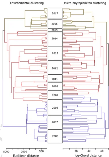
The concomitance of 2 major interannual changes was identified be-tween “environmental” and “microphytoplankton community” datasets using chronological clustering, leading to the distinction of 3 periods

(P⁠1, P⁠2and P⁠3) (Fig. 2). First change was observed during late-fall 2008

and spring 2009 and a second during winter 2015 and at the end of 2015, in environmental and microphytoplankton datasets respectively (see appendix D). Despite the uncertainty about the timing of the sec-ond change point in microphytoplankton composition due to a lack of data during 2015, PERMANOVA analysis indicated the significance of the partitioning (pval<0.01) (Table 2). However, the partitioning ex-plained less the total variance rather than annual or interannual

vari-ability (R⁠2_{=6, 13 and 17% respectively for “Period”, “Months” and}

“Years” factors, respectively).

3.2. Environmental variability and nutrients

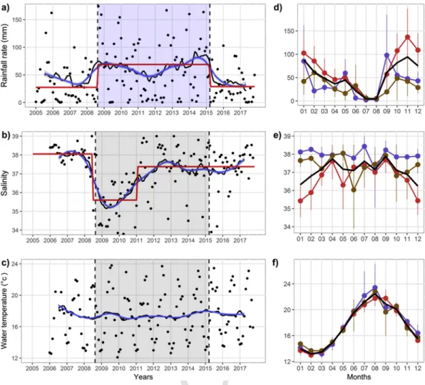
Analysis of univariate environmental data showed that period

parti-tioning was primarily driven by changes in the rainfall rate (Fig. 3a). P⁠1

was characterized by a relative low precipitation rate (∼27±48mm), associated with a high and stable salinity in the Large Bay

(∼38.1±0.5). Conversely, P⁠2 showed an increase of rainfall

(∼68.8±59.9mm), particularly during winter 2008/2009 which led to a brutal and persistent decrease of salinity in the Large Bay (∼35.6±1.2) detected from the end of 2008 until early 2011. Despite the maintenance of a high rainfall rate over the period 2009–2015, the increase in salinity trend was observed in 2011 and has conserved a rel-ative steady state until the end of 2017 (∼37.4±1.19) (Fig. 3b). Finally, from early 2015 rainfall rate showed a significant and sudden reduction until the end of 2017 (∼28.9±28.6mm). Seasonal variations in rainfall rate described a classical Mediterranean precipitation pattern with low-est values during summer and higher during late-fall/early-winter sea-son (mean of 4.5 and 88.1mm, respectively). The latest seasea-son was

par-ticularly impacted by the intensification of rainfall rate during P⁠2(mean

of 114±15mm between October to January) (Fig. 3d). Similarly, high-est differences in salinity between periods were found during the cold season (from November to February, mean of 38.1, 35.8 and 37.5 for

P⁠1, P⁠2and P⁠3, respectively) (Fig. 3e).

Fig. 2. Comparison of the chronological clusterings performed on the 2006–2017

“en-vironmental” dataset (water temperature, salinity and rainfall rate) using euclidean dis-tance (left cluster) and on the 2005–2017 “micro-phytoplankton community” dataset us-ing log-Chord distance (right cluster). For each dataset, colored branches identified 3 ho-mogeneous periods (P⁠1, P⁠2, and P⁠3in blue, red and brown) extracted from the 2 main

change points (Cut-off levels at h=[3658; 3429] and h=[67.2; 64.4] for the “environ-mental” and the “micro-phytoplankton” time series, respectively). Asymmetry between year boxes was relative to missing values in biological time-series. (For interpretation of the references to color in this figure legend, the reader is referred to the Web version of this article.)

Table 2

Summary of PERMANOVA analysis testing the influence of the partitioning (Periods), months (Months), years (Years), and their interaction (Months x Years) on log-chord distance of micro-phytoplankton abundance dataset. Df: degree of Freedom. SS: Sum of Squares. F.Model: F statistic from the permutation procedure.

Df SS F.Model R⁠2 _P-value Periods 2 4.40 13.4 0.06 *** Months 11 9.20 2.55 0.13 *** Years 12 12.09 3.07 0.17 *** Months x Years 94 40.33 1.31 0.56 *** Residuals 0.09 ***p < 0.001.

Based on incomplete time-series, no significant change were found between 2005 and 2006 (P1) and 2009 early 2010 (P2), nor between

2009 and 2010 (P2) and 2015 (P⁠3) in N-NO⁠x⁠- (mean of 2.4±4.5;

0.54±0.69 and 1.25±0.88μmoll⁠−1_{, respectively) and P-PO}

⁠4⁠3-(mean

of 0.09±0.03; 0.03±0.02 and 0.05±0.04μmoll⁠−1_{, respectively)}

con-centrations (Fig. 4a and b). P-PO⁠4⁠3- annual mean variations showed

UNCORRECTED

PROOF

Fig. 3. 2005–2017 time series of rainfall rate (a), salinity (b), and water temperature (c). Moving average (solid black line) and loess filter regression (α=0.3) (blue line) were performed

on raw data (black dots) to summarize the trend. Significant mean changes were indicated by red segments. Shaded area indicated (P⁠2) wet period delimited by change points (vertical

dotted lines) from environmental clustering. Respective mean annual variations (d, e and f) over the 2005–2017 (dark thick line) and the monthly averaged value with non-parametric 0.95 confident interval during each extracted period (blue, red and brown for P⁠1, P⁠2and P⁠3, respectively). (For interpretation of the references to color in this figure legend, the reader is

referred to the Web version of this article.)

June and July with no clear phenological signal (Fig. 4 d). Conversely,

N-NO⁠x⁠-concentrations showed a noticeable annual pattern with

min-ima found during late spring/summer (mean of 0.26μmoll⁠−1_between

May and August) and higher concentrations found in September (mean

of 4.8±9.2 μmoll⁠−1_{) and winter (mean of 3.3±1.8μmoll}⁠−1_between

January and March) (Fig. 4c). These two latter peaks were present in

(P⁠1) 2005–2006 (3.1±3.2 and 6.6±11.2μmol.l-1, respectively) and in

(P⁠3) 2015 data (2.3 and 2μmoll⁠−1, respectively) but absent during (P⁠2)

2009–2010 (0.5±0.4 and 0.2μmoll⁠−1_{, respectively). Furthermore, P}

⁠2 seasonal mean variation exhibited lower concentration values for both nutrients. Finally, water temperature didn't show significant change (p>0.05) in the mean (∼17.5°C) despite a strong seasonal variability with maximum values occurring in August (21.7±1.7°C) and minimum in February (13.2±0.4°C) in the 3 periods (Fig. 3c and f).

3.3. General phytoplankton composition 3.3.1. Total microphytoplankton abundance

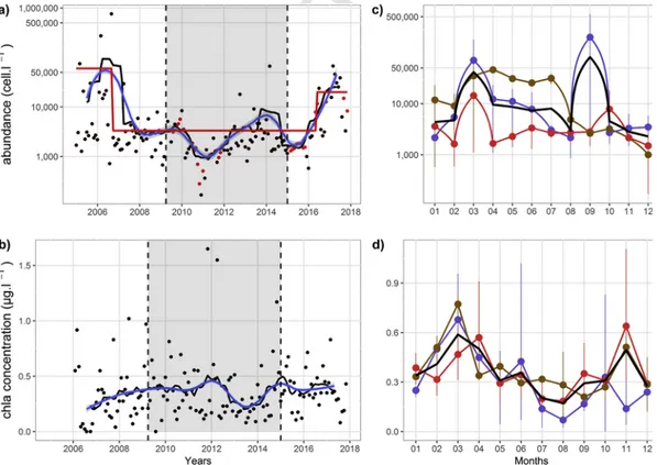
Total microphytoplankton abundance showed a high range of

val-ues from 168 to 7.6.10⁠5_cells.l⁠−1_{, during December 2010 and August}

2006, respectively with an average of 1.3.10⁠4_cells.l⁠−1 _{(Fig. 5a). The}

“Binary segmentation” method identified two significant change points

identifying 2005–2006, 2007–2014 and 2015–2017 subperiods. The first change occurred during early spring 2007 while the second ap-peared in early winter 2015 and coincided with the second change in partitioning analysis (Fig. 2). The 2005–2006 subperiod was

charac-terized by a higher average abundance (6.10⁠4_cells.l⁠−1_{) and contrasted}

with lowest average abundance observed during 2007–2014 period

(3.10⁠3_cells.l⁠−1_{). Finally, second change point was characterized by an}

increase of total abundance during the 2015–2017 subperiod (mean of

2.10⁠4_cells.l⁠−1_{). The latter did not show any significant difference with}

the 2005–2007 subperiod (pval>0.05). Clear seasonal pattern was ob-served over the 2005–2017 period characterized by 2 seasonal blooms

occurring in March (4.10⁠4_cells.l⁠−1_{) and September (8.10}⁠4_cells.l⁠−1_{) and}

with lowest values found in December (2.10⁠3_cells.l⁠-_{1) and August}

(3.10⁠3_cells.l⁠-_{1) (Fig. 5c). Global lower average values were observed}

during P⁠2, except in October showing higher values than average (mean

of 7.8.10⁠3_cells.l⁠−1_{). March abundance peak was identified during each}

period with high confident interval describing an inter-annual variabil-ity of bloom events. Nonetheless the highest bloom values were found

during P⁠1(7.10⁠4 in [1.10⁠3; 1.7.10⁠5] cells.l⁠−1) and weakest during P⁠2

(1.4.10⁠4_{in [1.10}⁠3_{; 4.10}⁠4_{] cells.l}⁠−1_{). Similarly, late-summer peak was}

only found during P⁠1(2.10⁠5in [3.10⁠3; 5.7.10⁠5] cell.l⁠−1) and was

miss-ing durmiss-ing P⁠2and P⁠3(2.8 in [1.10⁠3; 4.10⁠3] and 2.6.10⁠3in [1.10⁠3; 4.10⁠3]

UNCORRECTED

PROOF

Fig. 4. 2005–2017 N-NO⁠x⁠-and P-PO⁠4⁠3-time series (a and b, respectively) and annual variations (c and d, respectively) over the 2005–2017 period and mean monthly values from P⁠1,

P⁠2and P⁠3(blue, red and brown, respectively) with non-parametric 0.95 confident interval. Shaded area indicated (P⁠2) wet period delimited by change points (vertical dotted lines) from

environmental clustering. (For interpretation of the references to color in this figure legend, the reader is referred to the Web version of this article.)

Figure 5. 2005–2017 monthly time series of the total micro-phytoplankton abundance (a) with original (black dots) and interpolated data (red points) and chlorophyll a concentration

(b). Moving average (solid black line) and loess filter regression (α=0.3) (blue line) were performed on data to summarize the trend. The red segment indicated significant change in the mean. Vertical dashed line identified change points from biological partitioning and shaded area correspond to (P⁠2) wet period. Dark thick lines were for monthly averaged variations

of total micro-phytoplankton abundance (c) and chlorophyll a concentration (d) over the 2005–2017 period. Color lines described monthly averaged values with non-parametric 0.95 confident interval associated at each extracted period (blue. red and brown for P⁠1. P⁠2and P⁠3, respectively). Total abundance was expressed in log10 scale.

UNCORRECTED

PROOF

Chlorophyll a concentration described a phenological pattern with 2 annual concentration peaks during March–April (mean of

0.59±0.26μg. l⁠−1_{) and in November (mean of 0.49±0.46μgl}⁠−1_{) (Fig.}

5d). Globally, all periods showed spring blooms with higher values

found in March during P⁠3 and P⁠1 (mean of 0.77±0.08 and

0.68±0.33μgl⁠−1_{, respectively) and in April during P}

⁠2 (mean of

0.47±0.22μgl⁠−1_{). Otherwise, the November peak was only identified}

during P⁠2and P⁠3(0.64±0.56 and 0.51±0.11μgl⁠−1). No significant

dif-ference was observed between periods (pval>0.05).

Despite the absence of significant change in mean values, loess re-gression on moving average trend showed a gradual increase of the phytoplankton biomass in early 2008 (from 0.28±0.26 to

0.41±0.33μgl⁠−1_{) (Fig. 5b). The most important change in trend}

ob-served was a decrease of the chlorophyll a concentration from spring

2012 to fall 2014 (from 0.41±0.22 to 0.25±0.14μgl⁠−1_{). Finally, both}

loess regressions (α=0.3) on total abundance and on chlorophyll a concentration showed significant negative spearman correlation (rho=−0.61, pval <0.01).

3.3.3. Microphytoplankton composition

Diatoms were dominant in total microphytoplankton abundance, during the whole 2005–2017 period (53.3% on average) as well as in

the three extracted periods (61.1%, 57.3% and 39.8%, for P⁠1, P⁠2and

P⁠3, respectively) mostly due to the main representative taxa: P.

delicatis-sima, Chaetoceros spp., Cyclotella spp., Thalassionema spp. and L.danicus

(Table 1). Dinoflagellate group was the second most represented,

es-pecially during P⁠2(∼31%), driving by abundant species (e.g. C. furca,

P. micans, P.arcuatum, Alexandrium spp.). However, the most abundant

dinoflagellate taxa Gymnodinium spp. showed the highest mean

contri-bution during P⁠3(10.2%). Globally microflagellates were less abundant

over the 2005–2017 period (14.2%) but were identified as the second

contributor in total abundance during P⁠3(34%) driven by abundant

au-totrophic species H. fusiformis and Chlorella sp. (12.2 and 6.8%, respec-tively).

3.4. Changes in microphytoplankton assemblage

Among the 57 selected taxa, 21, 13 and 23 were respectively

as-sociated to P⁠1, P⁠2and P⁠3from the single IndVal⁠g index (Table 3). P⁠1

community was mostly composed of diatoms (13 out of 26 diatom taxa selected) and mixo/heterotrophic microflagellates (8 out of 15) (Table 1). Among the most abundant taxa, it was possible to mention

Chaeto-ceros spp. (0.83), L. danicus (0.76), D. fragilissimus (0.60), B. delicatulum

(0.50), H. hauckii (0.49) for diatoms and Leucocryptos sp. (0.59),

Chlamy-domonas sp. (0.44), Chromulina sp. (0.40) for microflagellates. Some

di-noflagellates species as Scripssiella sp., Achradina sp., Corythodinium sp. and small Protoperidinium spp. also exhibited high but not significant association values (0.56; 0.42; 0.33 and 0.31, respectively). Combined

IndVal⁠g_{index, which allowed an association of 2 periods, showed that}

some of P⁠1indicator taxa such as Chaetoceros spp., Chlamydomonas sp.,

Thalasionema spp. displayed higher association values for P⁠1and P⁠3

com-bination (0.86; 0.45 and 0.85, respectively).

Conversely, 10 of the 23 dinoflagellate taxa were significantly

asso-ciated to P⁠2and particularly P. arcuatum (0.80), C. furca (0.72), C. fusus

(0.57), P. divergens (0.48), Gonyaulax sp. (0.43), large Protoperidinium spp. (0.40) and P. pentagonum (0.39). Some diatom taxa such

Actinop-tychus sp. and in a less extent Coscinodiscus spp. were also associated

with P⁠2(0.73 and 0.48, respectively). Among these P⁠2indicators, some

dinoflagellates such as C. fusus, P. divergens, Gonyaulax sp. or D.

acumi-nata were more associated with the “P⁠2& P⁠3” combination. Only the

dinoflagellate species C.furca (0.77) and the diatom taxa Coscinodiscus

spp. (0.60) showed association with P⁠1and P⁠2. In addition, ANOSIM

Table 3

Summary of single and combined association measure (IndVal⁠g_{) of representative}

mi-crophytoplankton taxa with statistical significance of indexes: * <0.05; ** <0.01; *** <0.001.

Single Combined Taxa Class Period IndVal⁠g _{Period IndVal}⁠g

Chaetoceros spp. Diatom 1 0.834* 1 + 3 0.868* Leptocylindrus danicus Diatom 1 0.756*** 1 0.756** Dactyliosolen fragilissimus Diatom 1 0.600** 1 0.600** Leucocryptos sp. Flagellate 1 0.593** 1 0.593** Bacteriastrum delicatulum Diatom 1 0.500** 1 0.500** Hemiaulus hauckii Diatom 1 0.486** 1 0.486**

Chlamydomonas sp. Flagellate 1 0.444* 1 + 3 0.45* Chromulina sp. Flagellate 1 0.397* 1 0.397* Thalassionema spp. Diatom 1 0.728 1 + 3 0.848 * Scrippsiella spp. Dinoflagellate 1 0.559 1 + 3 0.69 Pseudonitzschia delicatissima Diatom 1 0.552 1 + 2 0.694 Achradina spp. Dinoflagellate 1 0.423 1 + 3 0.594 Asterionellopsis glacialis Diatom 1 0.413 1 0.413 Pseudonitzschia seriata Diatom 1 0.392 1 + 3 0.448 Skeletonema costatum Diatom 1 0.39 1 0.39 Gyrosigma sp. Diatom 1 0.35 1 + 2 0.402 Corythodinium sp. Dinoflagellate 1 0.328 1 + 3 0.382 Heterosigma sp. Flagellate 1 0.323 1 + 3 0.367 small Protoperidinium spp. Dinoflagellate 1 0.312 1 + 3 0.486 Fragilariopsis cylindrus Diatom 1 0.167 1 0.167 Lioloma sp. Diatom 1 0.143 1 + 2 0.156 Prorocentrum arcuatum Dinoflagellate 2 0.795*** 2 0.795*** Actinoptychus spp. Diatom 2 0.726*** 2 0.726***

Ceratium furca Dinoflagellate 2 0.722*** 1 + 2 0.766 **

Ceratium fusus Dinoflagellate 2 0.565* 2 + 3 0.587*

Protoperidinium divergens Dinoflagellate 2 0.483* 2 + 3 0.544* large Protoperidinium spp. Dinoflagellate 2 0.398* 2 + 3 0.489 ** Protoperidinium pentagonum Dinoflagellate 2 0.388* 2 0.388* Coscinodiscus spp. Diatom 2 0.486 1 + 2 0.608 Dinophysis acuminata Dinoflagellate 2 0.374 2 + 3 0.467 * Amylax spp. Dinoflagellate 2 0.325 2 + 3 0.371 Ceratium penatogonum Dinoflagellate 2 0.32 1 + 2 0.354 Gonyaulax spp. Dinoflagellate 2 0.282 2 + 3 0.466 Pseudonitzschia sp. Diatom 2 0.194 2 0.194 Rhodomonas sp. Flagellate 3 0.932*** 3 0.932***

Hillea fusiformis Flagellate 3 0.930*** 3 0.930***

Chlorella sp. Flagellate 3 0.922*** 3 0.922*** Gymnodinium spp. Dinoflagellate 3 0.895*** 1 + 3 0.969 *** Cyclotella spp. Diatom 3 0.884** 2 + 3 0.923 *** Nitzschia spp. Diatom 3 0.839*** 3 0.839*** Gyrodinium sp. Dinoflagellate 3 0.830*** 3 0.830*** Navicula spp. Diatom 3 0.784*** 3 0.784*** Guinardia spp. Diatom 3 0.749** 3 0.749** Prorocentrum micans Dinoflagellate 3 0.743** 2 + 3 0.754 ** Hemiselmis sp. Flagellate 3 0.720*** 3 0.720*** Oxytoxum spp. Dinoflagellate 3 0.688** 2 + 3 0.711 ** Amphidinium spp. Dinoflagellate 3 0.606** 3 0.606** Alexandrium spp. Dinoflagellate 3 0.593** 3 0.593**

UNCORRECTED

PROOF

Single Combined Taxa Class Period IndVal⁠g _{Period IndVal}⁠g

Licmophora gracilis Diatom 3 0.575** 3 0.575**

Tetraselmis spp. Flagellate 3 0.533* 1 + 3 0.54 * Pleurosigma sp. Diatom 3 0.526** 3 0.526** Thalasiosira spp. Diatom 3 0.522** 1 + 3 0.540 * Cylindrotheca closterium Diatom 3 0.618 1 + 3 0.799*** Dictyocha spp. Flagellate 3 0.575 1 + 3 0.758 ** Rhizosolenia spp. Diatom 3 0.467 1 + 3 0.511 Goniodoma sp. Dinoflagellate 3 0.393 2 + 3 0.490 ** Protoperidinium pellucidum Dinoflagellate 3 0.32 2 + 3 0.430 **

analysis identified dinoflagellates as the most impacted group by com-munity changes particularly in spring and summer (see appendix A, for details).

Finally, P⁠3was mainly associated with autotrophic microflagellates

species (e.g. Rhodomonas sp. (0.93), Hillea fusiformis (0.93), Chlorella sp. (0.92) but also with diatom taxa (e.g. Cyclotella spp. (0.88), Nitzschia spp. (0.84), Navicula sp. (0.78), Guinardia spp. (0.75)) and some dinofla-gellates (e.g. Gymnodinium spp. (0.89), Gyrodinium sp. (0.83), P.micans. (0.74), Oxytoxum spp. (0.68)).

3.5. Biovolumes and lifeform variations

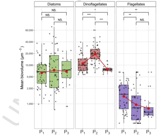
Globally, the dinoflagellate community described higher mean cell

biovolumes with values ranging from 1.10⁠4_{to 2.10}⁠4_μm⁠3_{(for Q25 and}

Q75, respectively) during the whole 2005–2017 period (Fig. 6). Diatom

mean cell biovolumes were, in turn, ranged between 6.2.10⁠3 _and

1.3.10⁠4_μm⁠3_{(for Q25 and Q75, respectively) and finally,}

microflagel-late community was constituted by lower cell sizes varying between

684 and 2.6.10⁠3_μm⁠3_{(for Q25 and Q75, respectively). Contrary to}

di-atom community, dinoflagellates and microflagellates exhibited signif-icant change of mean cell biovolumes between periods (pval<0.05). Thus, dinoflagellates described an increase of mean cell biovolumes

be-tween P⁠1and P⁠2(from 1.3.10⁠4to 2.2 .10⁠4μm⁠3, respectively) and then

a decrease in P⁠3(mean of 7.9.10⁠3μm⁠3), suggesting an important shift

within the community. Microflagellates only showed a significant

de-crease of mean cell biovolume between P⁠1 and P⁠2 (from 2.2.10⁠3to

1.7.10⁠3_μm⁠3_{, respectively), and then conserved low cell sizes during P}

⁠3

(mean of 1.1.10⁠3_μm⁠3_{). As none significant change in mean biovolumes}

was found for diatoms, the whole diatom community was subsequently considered as a unique lifeform. Conversely, these results led to the con-sideration of two different lifeforms for dinoflagellates characterizing species with biovolumes lower (small dinoflagellates) and higher (large

dinoflagellates) than 1.5.10⁠3_μm⁠3_{(see appendix C, for methodological}

details).

Mean seasonal anomalies of lifeform abundances described different interannual variations over the 2005–2017 period (Fig. 7). First, spring and summer diatom abundances increased mostly during years hosting intense wintering deep mixing in Ligurian Sea (+0.27, +1.59 and in a less extent −0.12 for 2005, 2006 and 2013, respectively) and also in 2017 (+0.63) for which there is no current report in the literature. Spring and summer anomalies of large dinoflagellates were positive

dur-ing P⁠2wet period (mean of +0.57 and + 0.72, respectively) except

during spring 2013 (−0.35). In addition, large dinoflagellate variations were negatively correlated to diatoms during spring (rho = -0.91) (see the summary in appendix E). Then, accordingly to seasonal anomalies,

Fig. 6. Mean cell biovolume variations of diatom (left panel), dinoflagellate (middle panel) and micro-flagellate (right panel) communities during the 3 extracted periods (P⁠1, P⁠2and P⁠3).

Black dots were for data, red point indicated averaged values during each period and red line summarized changes in mean. Boxplot indicated values ranged between the 25 and 75th percentile and median values. Results for Wilcoxon pairwise comparison using Bonferroni correction were specified: NS: no significant. * <0.05, ** <0.01, *** <0.001. Values were represented in 10 log scale. (For interpretation of the references to color in this figure legend, the reader is referred to the Web version of this article.)

UNCORRECTED

PROOF

Fig. 7. 2005–2017 standardized anomaly variations of diatom (Diat), microflagellate (Flag), large dinoflagellate (L.Dino) and small dinoflagellate (s.Dino) lifeforms. Annual mean

anom-alies (colored points) were computed from monthly anomalie values (black points) for winter (JFM), spring (AMJ), summer (JAS) and fall (OND). Shaded area corresponded to (P⁠2) wet

period. The years reported in the literature as they hosted intense wintering deep mixing in Ligurian Sea were indicated in bold red (ref(Heimbürger et al., 2013; Marty and Chiavérini, 2010; Pasqueron de Fommervault et al., 2015):). (For interpretation of the references to color in this figure legend, the reader is referred to the Web version of this article.)

microflagellate and small dinoflagellate abundances showed significant correlation in all seasons except in spring, despite a maximum abun-dance found in spring 2017 for both of them (+2.84 and + 2.87, re-spectively). With an exception for summer showing negative anomalies

during rainy periods, no clear impact of wet period (P⁠2) was observed

on abundances for both microflagellates and small dinoflagellates. Large and small dinoflagellate also showed a significant negative correlation during spring and summer (rho=−0.62 and −0.74). Finally, microfla-gellate and diatom variations showed significant positive correlation during winter (rho=0.58).

4. Discussion

Located in a deep convection area and nearby a large agglomera-tion, the semi-enclosed Toulon Bay was relevant to investigate the evo-lution of Mediterranean marine coastal systems confronted to both cli-matic and anthropogenic perturbations. The monitoring of plankton in Toulon Bay was already used to study annual variability of zooplank-ton (Jamet et al., 2001; Richard and Jamet, 2001), microphytoplank-ton (Boge et al., 2006; Jamet et al., 2005; Rossi and Jamet, 2009) and pico-nanophytoplankton (Delpy et al., 2018) as well as to identify local water indicators of anthropogenic pressure (Serranito et al., 2016). By using long-term time series, the present study focuses on decadal vari-ability (2005–2017) of the microphytoplankton community structure, to evaluate the impact of local and large-scale perturbations on coastal sys-tems.

4.1. Microphytoplankton assemblage features

Previously cited in 1999–2000 (Jamet et al., 2005) and 2006–2007 (Rossi and Jamet, 2009) annual cycles in Toulon Bay, representative taxa selected were also characteristic of the coastal NW Mediterranean basin. Abundant diatoms such as Chaetoceros spp., Thalasionema spp. or

Pseudonitzschia spp. were, in agreement with typical blooming genera,

dominant in deep convections areas (Siokou-Frangou et al., 2010). Al-though it remained less frequently reported, selective dinoflagellate taxa such as C. furca, P. micans, Gymnodinium spp., or Protoperidinium spp. were commonly associated with summer oligotrophic period (Gómez and Gorsky, 2003) and particularly in shallow anthropized areas (Garrido et al., 2014; Vila and Maso, 2005). It should be noticed that among dinoflagellate representative taxa, five were reported as poten-tially toxic (i.e. D. acuminata, P. micans, Alexandrium spp., Gonyaulax spp., and Gymnodinium spp.) (Faust and Gulledge, 2002; Ignatiades and Gotsis-Skretas, 2010; Mohamed, 2018).

4.2. Drivers of changes

Asynchronous qualitative and quantitative changes in microphyto-plankton communities were detected during the 2005–2017 period. A significant increase of wintering rainfall rate from late 2008 associated with a catastrophic change in salinity was followed during the next spring by the most important change among representative commu-nities according to chronological clustering (Figs. 2 and 3). It should be noticed that the accuracy of change points is a well-known issue in regime shift studies, as it depends on the length and regularity of time-series used. Hence, the absence of data during most of 2015 led to the detection of the second change point from the end of 2015, rather than during the expecting previous spring. Investigations on total mi-crophytoplankton abundance revealed higher values during dry periods,

i.e. from 2005 to late spring 2006 which coincide with major wintering

deep mixing events reported in Ligurian Basin (Heimbürger et al., 2013; Marty and Chiavérini, 2010) and during spring 2016 to the end of 2017 (Fig. 5).

Thenceforth, investigations on community changes pointed out two different aspects: (1) diatom and microflagellate taxa were mainly as-sociated to dry periods (Table 3). Diatom community was furthermore promoted during springs following convection event in Ligurian open sea (Fig. 7). Only diatom taxa Actinoptychus spp. showed an association

UNCORRECTED

PROOF

atoms as recently described by Kemp and Villareal (2018). (2) For di-noflagellate taxa, analysis identified two lifeforms involved in the main

community changes: while small dinoflagellates (<1,5.10⁠4_μm⁠3_{) were}

also associated with dry periods, following microflagellate variations,

the less abundant large dinoflagellate taxa (>1,5.10⁠4_μm⁠3_{) were favored}

by wet period (P⁠2).

These findings argued that changes in precipitation regime was the main driver of community changes during the 2005–2017 period, act-ing through different but superimposed processes at different scales: (1) a local wintering precipitation effect by runoff influence and (2) a re-gional precipitation deficit effect which mainly promoted vertical mix-ing.

4.3. Impact of local precipitation

4.3.1. Impacts on microphytoplancton community

In Toulon Bay, concomitant increase of rainfall regime and quali-tative changes in microphytoplankton communities assumed impact of terrestrial runoff on community assemblage. This community change was first characterized by a shift in mixotrophic/heterotrophic dinofla-gellate community, particularly during spring and summer (see

appendix A), promoting the large size taxa (>1,5.10⁠4_μm⁠3_{) at the}

ex-pense of smaller ones. Such a shift in size structure of heterotrophic communities also suggested a change in the nature of available preys. As pointed out by significant positive correlations, small dinoflagel-lates were highly associated to small size microflageldinoflagel-lates assuming a predator-prey relationship (appendix E). This hypothesis is in agree-ment with reports about trophic preference of mixotrophic and het-erotrophic dinoflagellates reported in scientific literature. For instance, it was shown that abundant species belonging to the small dinoflagel-late lifeform such as Gymnodinium spp. or P. micans, fed mainly on small size cryptophytes such as Teleaulax sp. (Jeong et al., 2010). Unlike other mixotrophic and heterotrophic dinoflagellates, armored Protoperidinium

spp. which were found highly associated with (P⁠2) wet period, executed

external digestion with an important range of size for its preys (Assmy and Smetacek, 2009; Buskey, 1997; Jacobson and Anderson, 1996). This extended diet included preferentially larger ones such as diatoms, di-noflagellates as well as ciliates (Jeong et al., 2010; Lee et al., 2014). Such feeding mechanisms allow them to modulate the classical preda-tor-prey allometric ratio of 10:1 (Azam et al., 1983). Protoperidinium genus was furthermore considered as an important opportunistic grazer of red-tide species, involved in their reduction (Jeong and Latz, 1994). Thus, high predation impact from large heterotrophic dinoflagellates on other smaller protists such as little dinoflagellates and diatoms, as previ-ously emphasized by Jeong et al. (2010), was consistent with the signif-icant negative correlation found between these lifeforms during spring and winter (Fig. 7). Although it was not considered in this study, the

in-crease of ciliate community during (P⁠2) wet period was suspected as low

abundances of diatoms and small dinoflagellates observed seemed insuf-ficient to support large dinoflagellate population growth. Furthermore, the widespread reported predation on ciliates from abundant large di-noflagellate C.furca (Ignatiades, 2012; Jeong et al., 2010; Smalley et al.,

2003; Smalley and Coats, 2002) (which was highly associated to (P⁠2)

wet period), also supported the increase of the ciliate population during

(P⁠2) wet period. Finally, for the poorly studied P. arcuatum, also

belong-ing to large dinoflagellates, mixotrophy and opportunistic nature was supported by the absence of correlation between abundance and nutri-ent concnutri-entration (Skejić et al., 2017).

4.3.2. Impacts on diatom community

Although diatom community was less impacted by the increase of

wintering rainfall rate during P⁠2than dinoflagellates (see appendix A),

main diatom taxa were associated to dry periods (P⁠1and P⁠3). Strict

au-totrophic siliceous diatoms are more sensitive to nutrient depletion or change in nutrient supply ratios than dinoflagellates, particularly for sil-icon (Si) (Anderson et al., 2002). It was assumed that diatoms were fa-vored in Si:N:P=16:16:1 conditions (Redfield et al., 1963) and that a variation from this ratio may result in a community shift toward non siliceous and smaller community (Cloern, 2001; Reynolds, 2006). For instance, a decrease in SI:N ratio in Bay of Brest between 1977 and 1995 due to an increase of anthropogenic nitrogen inputs from runoff, led to a limitation of the spring bloom intensity and an increase of hapto-phyta Phaeocystis sp. bloom (Chauvaud et al., 2000). Though nutrients (mainly nitrates) and organic matter as well as metallic contaminant were carried into Toulon Bay by Eygoutier River induced by heavy rain events (Nicolau et al., 2006), the relation between our increase of rain-fall and nutrient supply remained unclear due to the lack of data. How-ever, the reduction and the disappearance of the most abundant spring bloom diatom taxa as well as the silico flagellate Dictyocha sp. during

P⁠2suggested a nutrient depletion condition or a change in nutrient

sup-ply ratios. Also, as mixotrophic dinoflagellates were known to outcom-pete diatoms in organic nutrient conditions (Spilling et al., 2018), the change observed within the community may also suggest the impact of organic matter input from the Eygoutier River. It is interesting to note that such hypothesis contrast with the few available studies investigat-ing the impact of freshwater runoff on phytoplankton communities in coastal northwestern subbasin due to specific trophic state conditions. For instance, from shallow Blanes Bay station (Catalan coast) rainfall events were followed by an increase of diatom, dinoflagellate or crypto-phyte abundances as well as spring bloom intensity (Nunes et al., 2018). Similarly, in oligotrophic northern coastal Adriatic sea, the reduction of freshwater flow was identified as a driver of both change in phyto-planktonic composition, and reduction of total abundance during the 1986–2077 period (Aubry et al., 2012; Cabrini et al., 2012). Recently in the same region, a re-increase of the Pô river outflow observed during the 2007–2016 was followed by a reduction of coccolithophorid and by an increase in phytoflagellate biomass (Totti et al., 2019).

4.3.3. Impacts on chlorophyll a

In Toulon Bay, the absence of significant change in chlorophyll

a concentration at the decadal scale contrast with the total

micro-phytoplankton dynamic which followed mainly diatom variations. A significant negative correlation was furthermore found between their respective trends. As such, and although nanophytoplankton coccol-ithophorids were not investigated, chlorophyll a concentration would reflected mainly the nanophytoplankton dynamic rather than upper phytoplankton size class. As pointed out by Uitz et al. (2012), except during blooming periods, small size classes of phytoplankton (partic-ularly nanoplankon) contributed more to chlorophyll a concentration than microphytoplankton in NW Mediterranean Sea. Nanophytoplank-ton was also known to ‘overcompete’ other phytoplankNanophytoplank-ton classes in oligotrophic conditions (Siokou-Frangou et al., 2010), particularly due to a higher population growth rate and their ability to reduce the nutri-ent diffusion (Marañón, 2015). Thus, the contrasted dynamics between microphytoplancton and chlorophyll a also argue in favor of a shift in trophic conditions toward oligotrophy as a result of the increased rain-fall rate. This shift would lead, in turn to changes from diatom and mi-croflagellate dominance to smaller phytoplankton dominance-based sys-tem, which favored opportunistic large dinoflagellates.

4.4. Footprints from wintering deep mixings

Impact of wintering deep mixings was also observed in total micro-phytoplankton abundance as well as in diatom anomalies. During the early 2000s, deficit in freshwater budget caused by a low annual pre

UNCORRECTED

PROOF

events in the central Ligurian Sea, observed in 2005 and particularly in 2006 (Marty and Chiavérini, 2010). More recently, Coppola et al. (2018), reported at the DYFAMED point (central Ligurian Sea), a deep-ening of MLD during the winter 2013 suggesting a new but less in-tense, deep-mixing event. Concomitance between positive anomalies ob-served in diatom abundances during spring 2005, 2006 and 2013 (Fig. 7) and reported deep-mixings, supported the hypothesis of the influ-ence of regional mixing events on local microphytoplankton. Likewise,

high salinity and dry conditions observed in 2005–2007 period (P⁠1)

were in agreement with the increase of salinity and the deficit in pre-cipitation pointed out from the early 2000's in Ligurian Basin (Marty and Chiavérini, 2010). It would confirm the role of salinity as a power-ful indicator of large scale process in NW Mediterranean Sea (Somot et al., 2006). However, no coherent change or trend was identified in wa-ter temperature in Toulon Bay during the 2005–2017 period (Fig. 3c). Changes in water temperature has been also suspected as the main hy-drologic feature related to climate change and large scale processes in NW Mediterranean Sea (Goffart et al., 2015, 2002; Trigo and Davies, 2000; Vargas-Yáñez et al., 2010, 2008). We assumed that the absence of significant variability of water temperature in Toulon Bay during win-tering deep mixing events (i.e. decrease of Sea Surface Temperature) (Marty and Chiavérini, 2010) was probably due to both low water circu-lation into the bay and the impact of the local northern cold wind (Mis-tral). Second salty and dry period observed from early 2015 was also followed in winter and spring 2017 by an abrupt increase in total micro-phytoplankton abundance as well as positive anomalies in diatom and particularly in autotrophic microflagellates. Similarly to the beginning of 2000's, as low precipitation rate was observed in other meteorologi-cal stations around the Ligurian basin (i.e. Marseille, Nice and Calvi, see appendix F for details), a new freshwater deficit at a regional scale was suspected, leading to a potential new intense mixing event in 2017. Due to the absence of current reports, further investigations on late 2010s would be necessary to confirm occurrence of such a new deep mixing in Ligurian Sea as suggested by our biological responses and abiotic condi-tions.

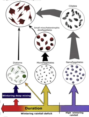
From the above discussion points, we produced a simplified model (Fig. 8) about the impact of rainfall on long term microphytoplank-ton dynamic in Toulon Bay, through two main mechanisms: 1) regional deep mixing events triggered by rainfall deficit, is the main fertiliza-tion driver of Toulon Bay, by shaping interannual variafertiliza-tions of microfla-gellate and particularly diatom spring bloom intensity. 2) the impact of wintering runoff intensification which promote smaller primary pro-ducer and lead to substantial changes in upper trophic levels such as in heterotrophic protists.

4.5. Community variability during dry periods

Although both dry and salty periods i.e. 2005–2008 (P⁠1) and

2015–2017 (P⁠3) shared assemblages dominated by diatoms and smaller

microflagellate taxa, numerous taxa were associated with only one of

them. Thus, P⁠1 appeared mainly associated with diatoms and some

heterotrophic flagellates whereas P⁠3was characterized by smaller

au-totrophic microflagellate (mainly cryptophyte species H.fusiformis) as

shown by IndVal⁠g(Table 3). Such pattern characterizing a second

al-ternation in primary producer nature may be driven by another no-table variability in nutrient supply during dry period. For instance, as the nutrient content of deep layers showed a decadal variability (Pasqueron de Fommervault et al., 2015), variations in the composi-tion of the nutrients provided by wintering mixing events could be con-sidered. Likewise, presence of instabilities from Northern Current in Toulon Bay (Guihou et al., 2013) could represent another local factor of nutrient enrichment, fueling punctual blooms (Casella et al., 2014)

Fig. 8. Simplified scenario of microphytoplanktonic ecosystem functioning in Toulon Bay

related to wintering rainfall variability. Arrows indicated highlighted (full black) and sus-pected (dashed grey) trophic relations between investigated (full circles) and not-inves-tigated (dashed circles) planktonic communities. Arrow thickness indicated the strength of relation supported by evidences. Rainy winters seemed favor small autotrophic cells (nanoflagellates) leading to important increase of large heterotrophic dinoflagellates sus-tained by ciliates. Dry winters promoted slightly abundant diatom and especially mi-cro-flagellate communities which were highly correlated with small mixotrophic dinofla-gellates. Both diatoms and small dinoflagellates may also be predated by larger dinoflagel-lates (mainly Protoperidinium spp.). Finally, rainfall deficit over several years was assumed as a driver of winter deep mixing at regional scale which triggered intense diatom spring blooms in Toulon Bay.

as pointed out in the French Riviera (Sammari et al., 1995; Taupier-Letage and Millot, 1986).

5. Conclusion

Using long-term monitoring time-series (2005–2017), the present study provides new insights on decadal microphytoplancton variations in a semi-enclosed and anthropized area, highlighting cell size as an im-portant descriptor of structure composition changes. Our data showed that precipitations were a keystone of microphytoplankton dynamics as it was involved in assemblage variations and bloom intensity: 1) Lo-cal wintering runoff was suspected to modify water nutrient supply ra-tio to the benefit of smaller and non-siliceous autotrophic communities such as nanophytoplankton and promoting opportunistic heterotrophic protists. 2) Regional rainfall deficit was identified as an important con-ditioning factor for wintering deep mixings in Ligurian Basin, and a key regulator of intense diatom and microflagellate spring blooms in the northern coast. Further investigations might be necessary to high-light suspected impacts of riverine on nutrient concentrations as well as consequences in upper trophic levels such as copepods. Further-more, our results support the idea that microphytoplankton composi-tion with an emphasis on size structure can be used as BQE regarding