HAL Id: hal-02398565
https://hal.archives-ouvertes.fr/hal-02398565
Submitted on 20 Nov 2020
HAL is a multi-disciplinary open access
archive for the deposit and dissemination of sci-entific research documents, whether they are pub-lished or not. The documents may come from teaching and research institutions in France or abroad, or from public or private research centers.
L’archive ouverte pluridisciplinaire HAL, est destinée au dépôt et à la diffusion de documents scientifiques de niveau recherche, publiés ou non, émanant des établissements d’enseignement et de recherche français ou étrangers, des laboratoires publics ou privés.
Evolution of specialization in heterogeneous
environments: equilibrium between selection, mutation
and migration
Sepideh Mirrahimi, Sylvain Gandon
To cite this version:
Sepideh Mirrahimi, Sylvain Gandon. Evolution of specialization in heterogeneous environments: equi-librium between selection, mutation and migration. Genetics, Genetics Society of America, In press. �hal-02398565�
Evolution of specialization in heterogeneous environments:
equilibrium between selection, mutation and migration
Sepideh Mirrahimi⇤ Sylvain Gandon†
Abstract
Adaptation in spatially heterogeneous environments results from the balance between local selection, mutation and migration. We study the interplay among these di↵erent evolutionary forces and demography in a classical two-habitat scenario with asexual reproduction. We develop a new theoretical approach that goes beyond the Adaptive Dynamics framework and allows us to explore the e↵ect of high mutation rates on the stationary phenotypic distribution. We show that this approach improves the classical Gaussian approximation and captures accurately the shape of this equilibrium phenotypic distribution in one and two-population scenarios. We examine the evolutionary equilibrium under general conditions where demography and selection may be non-symmetric between the two habitats. In particular, we show how migration may increase di↵erentiation in a source-sink scenario. We discuss the implications of these analytic results for the adaptation of organisms with large mutation rates such as RNA viruses.
Key-Words: local adaptation, migration-selection balance, gene flow, Adaptive Dynam-ics, Quantitative GenetDynam-ics, skew.
1
Introduction
Spatially heterogeneous selection is ubiquitous and constitutes a potent evolutionary force that pro-motes the emergence and the maintenance of biodiversity. Spatial variation in selection can yield adaptation to local environmental conditions, however, other evolutionary forces like migration and mutation tend to homogenize the spatial patterns of di↵erentiation and thus to impede the build up of local adaptation. Understanding the balance between these contrasted evolutionary forces is a major objective of evolutionary biology theory Slatkin 1978; Whitlock 2015; Savolainen et al. 2013) and could lead to a better understanding of the speciation process and the evolutionary response to global change Doebeli and Dieckmann 2003; Leimar et al. 2008. In this article, we consider a two-habitat model with explicit demographic dynamics as in Mesz´ena et al. 1997; Day 2000; Ronce and Kirkpatrick 2001; D´ebarre et al. 2013. We assume that adaptation is governed by a single quantitative trait where indi-viduals reproduce asexually. Maladapted populations have a reduced growth rate and, consequently, lower population size. In other words, selection is assumed to be ’hard’ Christiansen 1975; D´ebarre and Gandon 2010 as the population size in each habitat is a↵ected by selection, mutation and migration. These e↵ects are complex because, for instance, non-symmetric population sizes a↵ect gene flow and adaptation feeds back on demography and population sizes Nagylaki 1978; Lenormand 2002; Mesz´ena ⇤Institut de Math´ematiques de Toulouse, UMR5219, Universit´e de Toulouse, CNRS, UPS, IMT, F-31062 Toulouse Cedex 9, France
†CEFE UMR 5175, CNRS – Universit´e de Montpellier, Universit´e Paul-Val´ery Montpellier, EPHE, 1919, route de Mende, 34293 Montpellier Cedex 5, France
et al. 1997; Day 2000; Ronce and Kirkpatrick 2001; D´ebarre et al. 2013. To capture the complexity of these feed backs it is essential to keep track of both the local densities and the distributions of phe-notypes in each habitat. Note that this complexity often led to the analysis of the simplest ecological scenarios where the strength of selection, migration and demographic constraints are assumed to be the same in the two habitats (we will refer to such situations as symmetric scenarios). See however Holt and Gaines 1992; Garc´ıa-Ramos and Kirkpatrick 1997; Gomulkiewicz et al. 1999; Holt et al. 2003 for the analysis of the e↵ect of asymmetric migration from a source habitat on the dynamics of adap-tation in a peripheral (i.e. sink) habitat. Three di↵erent approaches have been used to analyze these two-population models. Each of these approaches rely on a set of restrictive assumptions regarding the relative influence of the di↵erent evolutionary forces acting on the evolution of the population. First, under the assumption that the rate of mutation is weak relative to selection, it is possible to use the Adaptive Dynamics framework (see Mesz´ena et al. 1997; Day 2000; Szil´agyi and Mesz´ena 2009; D´ebarre et al. 2013; Fabre et al. 2012 and also sections 3.1.1 and 3.2.1 for a presentation of this framework). This analysis captures the e↵ect of migration and selection on the long-term evolutionary equilibrium. In particular, this approach shows that weak migration relative to selection promotes the coexistence of two specialist strategies (locally adapted on each habitat). In contrast, when migration is strong relative to selection, a single generalist strategy is favored. The main limit of this approach is that it relies on the assumption that mutation rate is vanishingly small which results in a very limited amount of genetic variability. At most, 2 genotypes can coexist in this two-habitat model.
Second, Quantitative Genetics formalism, based on the computation of the moments of the phenotypic distribution, has been used to track evolutionary dynamics in heterogeneous habitats when there is substantial level of phenotypic diversity in each population Ronce and Kirkpatrick 2001. This model considers sexual reproduction with a quantitative trait (considering multiple loci with small e↵ects Fisher 1919). However, similar types of equations, describing the dynamics of the moments of the phenotypic distribution, can also be derived in the case of asexual reproduction considering large mutation rates (see D´ebarre et al. 2013 and Section 3.2). This formalism allows to recover classical migration thresholds below which specialization is feasible. But the analysis of Ronce and Kirkpatrick 2001 also reveals the existence of evolutionary bistability where transient perturbations of the demography can have long term evolutionary consequences on specialization. Yet, the assumption on the shape of the phenotypic distribution (assumed to be Gaussian in each habitat) is a major limit of this formalism.
Third, attempts to account for other shapes of the phenotypic distributions in heterogeneous environ-ments have been developed recently Yeaman and Guillaume 2009; D´ebarre et al. 2013, 2015. These models highlight that calculations based on the Gaussian approximation which neglects the skewness of the equilibrium phenotypic distribution under-estimates the level of phenotypic divergence and local adaptation. Yet, there is currently no model able to accurately describe the build up of non-Gaussian distributions. The only attempt to model this distribution is to describe the phenotypic distributions in each habitat as the sum of two Gaussian distributions Yeaman and Guillaume 2009; D´ebarre et al. 2013. These models, however, only yield approximate predictions on long-term evolutionary equilibria. Here we develop an alternative formalism that yields the population size and the phenotypic distri-bution in each habitat at the equilibrium between selection, mutation and migration. In Section 2 we present our two-population model.For heuristic reasons, we next provide the analysis of the equi-librium between selection and mutation in a single population. This provides an illustration of our approach in a simple scenario and shows how this analysis can go beyond the classical Gaussian ap-proximation. Next, we extend this approach to a two-population scenario where migration can also influence the phenotypic distribution, and we derive approximations for the level of adaptation under
a migration-selection-mutation balance. We also explore the e↵ects of non-symmetric constraints on selection, migration or demography between the two habitats. We evaluate the accuracy of these ap-proximations by comparing them to numerical solutions of our deterministic model and we show that our approach improves previous attempts to study the interplay between adaptation and demography in heterogeneous environments. We contend that our results are particularly relevant for organisms with high mutation rates and may help to understand the within-host dynamics of chronic infections by RNA viruses Drake and Holland 1999; Sanju´an et al. 2010.
The present work has been prepared in parallel to the mathematical article Mirrahimi 2017 where we provide the mathematical basis and proofs for the method used here. See also Gandon and Mirrahimi 2016 where those mathematical results were announced. The aim of the present paper is to show how this approach can help to understand the balance between di↵erent evolutionary forces. We present several new biological scenarios and we derive new results that help grasp the interplay between di↵erent evolutionary forces and demography.
2
Materials and Methods
We model an environment containing two habitats that we label 1 and 2 (Figure 1). The population is structured by a quantitative trait z. In each habitat i there is stabilizing selection on the trait z for an optimal value ✓i (for habitat i = 1, 2). The growth rate in habitat i is denoted by ri(z) which has its maximum rmax,i when z = ✓i. In the following we will mainly focus on the following quadratic stabilizing selection function (B¨urger 2000– pages 117-121 and chapter VI):
ri(z) = rmax,i si(z ✓i)2. (1)
We denote by si the selection pressure in habitat i. Without loss of generality we assume that ✓1 = ✓2 = ✓. But our approach could be used with other stabilizing selection functions (see (12) below where another selection function is studied in the case of one population).
Reproduction is assumed to be asexual. O↵spring inherit the phenotype of their parent (i.e. no envi-ronmental variance) and we consider a continuum of alleles model Kimura 1965. Mutations occur with a constant rate U (i.e. mutations are not associated with reproduction) and add an increment y to the parents’ phenotype; we assume that the distribution of these mutational e↵ects is given by K(y), with mean 0 and variance equal to 2Vm. We also assume that individuals disperse out of habitat i with rate mi. Rates of migration are assumed to be independent of individuals’ phenotypes.
Let ni(t, z) be the phenotypic density in habitat i at time t. The dynamics of this density in each habitat is given by (for i = 1, 2 and j = 2, 1):
@ni(t,z) @t = U Z +1 1 ni(t, z y)K(y)dy ni(t, z) | {z } mutation + ni(t, z) ✓ ri(z) i Z +1 1 ni(t, y)dy ◆ | {z } growth + mjnj(t, z) mini(t, z) | {z } migration . (2)
θ1 θ2 rmax,1 rmax,2 s1 s2 m1 FITNESS POPULATIONS μ1 μ2 phenotype z phenotype z differentiation
Figure 1 – Schematic representation of the 2 habitat model. The top figure shows the growth rate (fitness) in each habitat as a function of the phenotypic trait z. In habitat i the growth rate is assumed to be maximized at z = ✓i and the strength of selection is governed by si (see equation (1)). Here we illustrate a scenario with non-symmetric fitness functions. The bottom figure shows the phenotypic density in each habitat (light blue and light red in habitats 1 and 2, respectively). Migration from population i is governed by the parameter mi and tends to reduce the di↵erentiation (i.e. the di↵erence between the mean phenotypes) between populations.
second term corresponds to logistic growth that results from the balance between reproduction given by (1) and density dependance where i measures the intensity of competition within each habitat. The last term corresponds to the dispersal of individuals between habitats.
If we assume that the variance of the mutation distribution is small relative to the mutation rate U , we can consider an approximate model where we replace the mutation term in (2) by a di↵usion (see Kimura 1965; Lande 1975 and the more recent article Champagnat et al. 2008 where the di↵usion term has been derived directly from a stochastic individual based model). See also B¨urger 2000–pages 239-241 for a discussion on the domain of the validity of such model. Our model then becomes:
@ni(t, z) @t = U Vm @2n i(t, z) @z2 + ni(t, z) ✓ ri(z) i Z +1 1 ni(t, y)dy ◆ + mjnj(t, z) mini(t, z). (3) The total population sizes in each habitat is given by:
Ni(t) = Z +1
1
ni(t, z)dz, for i = 1, 2. (4)
In other words, ni(t, z) refers to the density of individuals with phenotype z in habitat i, while Ni refers to the total density of the polymorphic population in habitat i.
Data availability No biological data is provided in this article.
3
Results
3.1 One population: the selection-mutation equilibrium
In this section we start by a simple scenario with no migration. This one-population example provides a good introduction to our method. The dynamics of the phenotypic density in a single habitat is given by:
@n0(t, z)
@t = U Vm
@2n0(t, z)
@z2 + n0(t, z) (r0(z) N0(t)) , (5)
where N0 is the total population size:
N0(t) = Z +1
1
n0(t, y)dy.
For this scenario we consider a more general form of growth rate r0(z) than (1). We only suppose that r0(z) is maximized for an optimal trait z0. In the following we present our two-step approach. First, we analyse the evolutionary equilibria of the problem when the rate of mutation is small and we identify the evolutionary stable strategy (ESS). Second, we use this ESS to derive an approximation for the stationary solution of (5) when mutation is more frequent and maintains a standing variance at equilibrium.
3.1.1 Adaptive dynamics and evolutionary stable strategies
In this section, we assume that the mutations are very rare such that a mutation is fixed or goes extinct before a new mutation arises in the population. The phenotypic distribution results from a collection of spikes. Such spikes are gradually replaced by others with the arrival of new mutations and through a competitive procedure. The theory of Adaptive Dynamics Geritz et al. 1998 is based on the study of the stable equilibrium distribution and the localization of the spikes of such equilibrium, known as evolutionary stable strategies (ESS). Note that in this first step we do not make any assumption regarding the e↵ects of these mutations on the phenotype. We are interested in the identification of the global ESSs, i.e. when the resident population cannot be invaded by any mutation no matter its e↵ect.
In absence of migration, the phenotype z0 constitutes a globally stable evolutionary strategy. Indeed, when such monomorphic population reaches its demographic equilibrium, the total population size is given by N0⇤ = r(z0) . The fate of a mutant with phenotype zm introduced in such a resident population is determined by its fitness given by (i.e. per capita growth rate minus density dependence):
w(zm; N0⇤) = r0(zm) 0N0⇤ < w(z0; N0⇤) = 0. (6) No mutant trait zm can indeed invade the population since r0(z) takes its maximum at z0.
3.1.2 Equilibrium distribution with mutation
The ESS z0 corresponds to the long-term evolutionary outcome in a scenario where all phenotypic strategies are present initially but where mutation is absent. In the following we study the impact of
mutation on the ultimate evolutionary equilibrium of the population.
We introduce a new parameter " = pVm. Hence we replace Vm by "2 and we approximate the phe-notypic density n⇤",0(z), the equilibrium of (5), in terms of " (where the subscript " in n⇤",0 indicates the dependence of the phenotypic density on the parameter "). Our objective is to provide an ap-proximation of the phenotypic density when the e↵ect of mutation (measured by ") is small while the mutation rate can be large.
To study n⇤",0(z) we will use a method based on Hamilton-Jacobi equations (see equation (A.5)) which has been developed by the mathematical community during the last decade to study selection-mutation models, when the e↵ect of mutations is vanishingly small. This method was first suggested by Diek-mann et al. 2005 and was developed for the case of homogeneous environments in Perthame and Barles 2008; Barles et al. 2009. However those works, which are addressed to the mathematical community, were mainly focused on the limit case where the e↵ect of mutations " is vanishingly small. Here, we go further than previous studies and characterize the phenotypic distribution when the mutations have non-negligible e↵ects.
The method is based on the following transformation: n⇤",0(z) = p1 2⇡"exp ⇣u",0(z) " ⌘ . (7)
The introduction of the function u",0(z) is a mathematical trick. It is indeed easier to provide first an approximation of u",0(z) rather than directly studying n⇤",0(z).
Note that a first approximation of the population’s phenotypic density which is commonly used in the theory of Quantitative Genetics is a Gaussian approximation of the following form around z⇤:
n⇤",0(z)⇡ N",0⇤ N (z⇤, " 2). (8) The Gaussian approximation, is as if we had imposed u",0(z) to be a quadratic function of z, that is u",0(z) = " log(
N⇤ ",0
) (z z2 2⇤)2. Our objective, however, is to obtain more accurate results than (8) and to approximate u",0 without making an a priori Gaussian assumption. To this end we postulate an expansion for u",0(z) in terms of ":
u",0(z) = u0(z) + "v0(z) + O("2), (9) and we try to compute the coefficients u0(z) and v0(z). These terms can indeed be explicitly computed and they lead to an approximation of the total population size N"⇤ and the phenotypic density n⇤"(z) that we will call henceforth our first approximation (see the supplementary information A.1.1 for these derivations).
In order to provide more explicit formula for the moments of order k 1 of the population’s distri-bution in terms of the parameters of the model, we also provide a second approximation. This second approximation, instead of using the values of u0 and v0 in the whole domain, is based on the Taylor expansions of u0 and v0 around the ESS points (see the supplementary information, Section A.1.2). Our second approximation is by definition less accurate than the first one. We illustrate below the quality of these di↵erent approximations under two di↵erent scenarios.
Quadratic growth rate: We first consider a quadratic growth rate as in (1):
In this case our first approximation yields the Gaussian distribution (8) with: N",0⇤ ⇡ 1 0 (rmax,0 " p s0U ), 2 ⇡ p U ps 0 . (11)
Note that this Gaussian distribution is actually an exact equilibrium of (3) and the above⇡ signs can indeed be replaced by equalities (see Kimura 1965 and B¨urger 2000–Chapter IV). For the derivation of this result see the supplementary information–Section A.1.1.
An asymmetric growth rate: We next consider a growth rate which is not symmetric:
r0(z) = rmax,0 s0(z ✓0)2 a + (z ✓0 b)2 . (12)
In this case the phenotypic distribution does not have a Gaussian profile and our approximation yields: N",0⇤ ⇡ 1 0 (rmax,0 p s0U (a + b2) "), n⇤",0(z)⇡ 1 p 2⇡"exp ⇣u0(z) + "v0(z) " ⌘ ,
where the values of u0 and v0 can be computed explicitly (see the supplementary information–Section A.1.1). In Figure 2 we plot this first approximation and compare it with the exact distribution that we derived numerically.
We can also use our second approximation to obtain analytic expressions for the mean phenotypic trait (see the supplementary information-Section A.1.2 for the derivation):
µ⇤",0= 1 N",0⇤ Z zn⇤",0(z)dz = ✓0+ 2bpU " ps 0(a + b2)3/2 + O("2), the mean variance:
⇤2 ",0= 1 N⇤ ",0 Z (z µ⇤",0)2n⇤",0(z)dz = p U " p s0(a + b2) + O("2), and the third central moment:
⇤ ",0= 1 N",0⇤ Z (z µ⇤",0)3n⇤",0(z)dz = 2bU " 2 s0(a + b2)2 + O("3).
In Table 1 we show that our two approximations capture accurately the first three moments of the equilibrium distribution using the parameters that we used in Figure 2. As expected, the first approx-imation is more accurate, but the analytic expressions of the second approxapprox-imation given above allow us to capture the influence of the parameters of the model.
3.2 Two populations: the selection-mutation-migration equilibrium
Next we return to the analysis of the stationary solution of (3), which results from the equilibrium between selection, mutation and migration in each habitat. Using (1) and (3) one can derive dynamical
-1.5 -1 -0.5 0 0.5 1 1.5 Phenotypic trait z 0 0.5 1 1.5 2 2.5 3 3.5 Phenotypic density
Figure 2 – The selection-mutation equilibrium of the phenotypic density n",0(z) in a
single population. We plot the exact phenotypic density at equilibrium obtained from numerical computations of the equilibrium of (5) (blue dots) together with our first approximation (full black line) with the growth rate given in (12). The vertical dotted line indicates the mean of the phenotypic distribution. Note the skewness of the equilibrium distribution that is accurately captured with our approximation (see also Table 1). In this figure, to compute numerically the equilibrium, we have solved numerically the dynamic problem (5) and kept the solution obtained after long time when the equilibrium has been reached. Parameter values: rmax= 3, s0 = 1; ✓ = 0.5, = 1, a = 0.2, b = 1, U = 1, " = 0.1.
equations for the size of the population and the mean phenotype (µi = Ni1 R zni(t, z)dz): d dtNi = Ni(rmax,i iNi) siNi (µi ✓i) 2+ 2 i + mjNj miNi, d dtµi= si 2(µi ✓i) 2 i + i + mjNj Ni (µj µi), where 2
i and i are the variance and the third central moment of the phenotypic distribution, respec-tively. These two quantities are also dynamical variables and their dynamics are governed by higher moments of the phenotypic distribution. But this dynamical system is not closed and these higher moments are also dynamical variables that depend on additional moments. Various approximations, however, have been used to capture its behavior. Typically, many results are based on the Gaussian approximation that focuses on the dynamics of the mean and the variance and discards all higher cumulants of the distribution B¨urger 2000; Rice 2004. Yet several authors pointed out that neglecting the skewness of the distribution can underestimate the amount of di↵erentiation and local adaptation Yeaman and Guillaume 2009; D´ebarre et al. 2013, 2015. Indeed, in the case of symmetric habitats, that is when m1 = m2 = m, 1 = 2 = , s1 = s2 = s, rmax,1 = rmax,2 = rmax, one can readily obtain the size and the mean trait of the population at equilibrium (the equilibrium is indicated by a superscript⇤). Using the fact that N⇤
1 = N2⇤ = N⇤, µ⇤1 = µ⇤2, 1⇤= 2⇤= ⇤ and 1⇤ = 2⇤ = ⇤, we obtain: N⇤= 1 ⇣ rmax s⇣(2m✓ s ⇤)2 4(m + g ⇤ 2)2 + ⇤ 2 ⌘⌘ ,
Exact value First approximation Second approximation
Mean: µ⇤",0 -0.29 -0.29 -0.35
Variance: ",0⇤2 0.13 0.14 0.09
Third central moment: ⇤
",0 0.02 0.02 0.01
Table 1 – First three moments of the phenotypic distribution at mutation-selection equi-librium in a single population. We compare the values from the exact numerical resolution of (5) and our two approximations using the growth rate given in (12) (see also Figure 2). Parameter values: rmax= 3, s0 = 1; ✓ = 0.5, = 1, a = 0.2, b = 1, U = 1, " = 0.1.
µ⇤1 = s( ⇤+ 2✓ ⇤ 2) 2(m + s ⇤ 2) . The di↵erentiation between the two habitats is thus (Figure 1):
µ⇤2 µ⇤1 = s( ⇤+ 2✓ ⇤ 2)
m + s ⇤ 2 . (13)
There is, however, no analytic predictions on the magnitude of the di↵erent moments of the phenotypic distribution except in the limit when the mutation rate is extremely low D´ebarre et al. 2013.
Next, we follow the two-step approach we used to obtain the stationary phenotypic distribution in a single population. First, we analyse the evolutionary equilibria of the system when mutations are rare using the Adaptive Dynamics framework. We identify monomorphic or dimorphic globally evolu-tionary stable strategies (ESS). Second, we use these ESSs to derive approximations of the staevolu-tionary solution of (3) when mutation is more frequent and maintains a standing variance at equilibrium.
3.2.1 Adaptive dynamics and evolutionary stable strategies
We consider a resident population at a demographic equilibrium set by the phenotypic densities of the resident in both habitats (see the supplementary information, Section A.2.1.1). We want to determine the fate of a mutant with phenotype zm introduced in this resident population. The ability of the mutant to invade is determined by its fitness given by:
wi(zm; Ni) = ri(zm) iNi, for i = 1, 2. (14)
To take into account migration between habitats we introduce an e↵ective fitness which corresponds to the growth rate of a trait in the whole environment (see Caswell 1989; Metz et al. 1992; Mesz´ena et al. 1997). The e↵ective fitness W (zm; N1, N2), which corresponds to the e↵ective growth rate associated with trait zm in the resident population (n1, n2), is the largest eigenvalue of the following matrix:
A(zm; N1, N2) = ✓ w1(zm; N1) m1 m2 m1 w2(zm; N2) m2 ◆ . (15)
After some time, the dynamical system will reach a globally stable demographic equilibrium. Because there are two habitats, we expect that at most two distinct traits can coexist. With an analysis of the e↵ective fitness W , we characterize such equilibrium corresponding to the evolutionary stable strategy (see the supplementary information, Section A.2.1.1). This equilibrium is indeed either monomorphic (with phenotype zM⇤and the total population size NiM⇤) or dimorphic (with phenotypes zID⇤ and zIID⇤ and the total population sizes NiD⇤, where the subscripts I and II indicate that the phenotype is best adapted to habitat 1 and 2, respectively).
3.2.2 Equilibrium distribution with mutation
In the following we allow mutation rate to increase and we study the impact of mutations on the ultimate evolutionary equilibrium of the phenotypic densities, i.e. the stationary solution of (3). We present below the general principle of the approach before examining specific case studies.
As in Section 3.1.2 we introduce the parameter " =pVm and we approximate the phenotypic density n⇤",i(z), the equilibrium of (3) with Vm = "2, in terms of ". Our objective is to provide an approxima-tion of the phenotypic density in each habitat when the e↵ect of mutaapproxima-tion (measured by ") is small while the mutation rate can be large.
We use analogous transformation to (7):
n⇤",i(z) = p1 2⇡"exp
u",i(z)
" . (16)
Our objective is then to estimate u",i(z). We proceed as in Section 3.1.2 and we postulate an expansion for u",i in terms of ":
u",i(z) = ui(z) + "vi(z) + O("2), (17) and we try to compute the coefficients ui(z) and vi(z) . First we can show that, when there is migra-tion in both direcmigra-tions (i.e. mi > 0 for i = 1, 2), the zero order terms are the same in both habitats: u1(z) = u2(z) = u(z) (see the supplementary information, Section A.2.1.2). We can indeed compute explicitly u(z) which is given by (A.23) in the monomorphic case and by (A.24) in the dimorphic case. As we observe in the formula (A.23) and (A.24), u(z) attains its maximum (which is equal to 0) at the ESS points identified in the previous subsection. This means that the peaks of the population’s distribution are around the ESS points (zM⇤ in the case of the monomorphic ESS and (zID⇤, zIID⇤) for the dimorphic ESS). Note that the fact that u1(z) = u2(z) = u(z) means that the peaks of the population distribution are placed approximately at the same points (ESS points) in both habitats. However, the size of the peaks may be di↵erent since v1(z) is not necessarily equal to v2(z).
We are also able to compute the first order term vi(z) (see the supplementary information, Section A.2.1.2). This allows us to obtain a first approximation of the phenotypic density n⇤",i(z). This ap-proximation of the stationary distribution is very accurate (see for instance Figure 4).
As in section 3.1.2 we derive more explicit formula for the moments of order k 1 of the stationary phenotypic distribution. This second approximation, instead of using the values of u(z) and vi(z) in the whole domain, is based on the computation of the Taylor expansions of u(z) and vi(z) around the ESS points (see the supplementary information, Section A.2.1.3).
3.2.3 Case studies
Symmetric fitness landscapes
We focus first on a symmetric scenario where, apart from the position of the optimum, the two habi-tats are identical: m1 = m2 = m, 1 = 2 = , s1 = s2 = s, rmax,1 = rmax,2 = rmax. In this special case it is possible to fully characterize the evolutionary equilibrium.
When migration rate is higher than critical migration threshold:
m > mc = 2s✓2 (18)
migration prevents the di↵erentiation of the trait between the two habitats (see the supplementary information- Subsection A.2.1.1). The only evolutionary equilibrium, when the mutation rate is van-ishingly small, is monomorphic and satisfies zM⇤= 0 and nM⇤
1 (z) = nM⇤2 (z) = NM⇤ (z), where (.) is the dirac delta function and NM⇤ = 1 rmax s✓2 .
Monomorphic case: Let’s suppose that mc = 2s✓2 m. Then zM⇤ = 0 is the only ESS and
NM⇤ = 1 rmax s✓2 . Then, we can provide our first approximation of the phenotypic density n",i(z) following the method introduced above (Figure 3). Moreover, defining =
p
1 2s✓2/m, we can use the second approximation to obtain analytic formula for the moments of the stationary state:
8 > > > > > > > > > < > > > > > > > > > : NM⇤ ",1 = N",2M⇤ = R nM⇤ ",i (z)dz = 1 rmax s✓2 " p U s + O("2), µM⇤ ",1 = N1M⇤ ",1 R znM⇤",1(z)dz = "pmU s ✓+ O("2), µM",2⇤= N1M⇤ ",2 R znM",2⇤(z)dz = "pmU s ✓ + O("2), M⇤ 2 ",1 = ",2M⇤ 2= N1M⇤ ",i R (z µM",i⇤)2nM",i⇤(z)dz = "ppU s + O(" 2), M⇤ ",i = N1M⇤ ",i R
(z µM",i⇤)3nM",i⇤(z)dz = O("3).
(19)
These results are consistent with (13). Note that the equilibrium variance in each habitat M⇤2 ",i ⇡ "
p U p
s is larger than the equilibrium variance maintained in the absence of heterogeneity between the habitats
(compare with (11)). This increase in the equilibrium variance comes from which depends on
dispersion and the heterogeneity between the two habitats. The variance of the distribution increases
as decreases. When = 0 the approximation for the variance becomes infinitely large. Indeed,
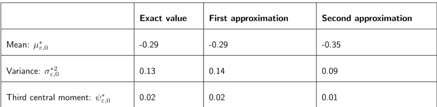
this corresponds to the threshold value of migration below which the above approximation collapses because the distribution becomes bimodal. In this case we have to switch to the analysis of the dimorphic case. Note that the di↵erentiation between habitats depends also on . Some di↵erentiation emerges even when the migration rate is above the critical migration rate, mc (Figures 3 and 4). In Figure 4 we provide a comparison of the results from the first and the second approximations. Our second approximation yields convincing results when the parameters are such that we are far from the transition zone from monomorphic to dimorphic distribution. This approximation is indeed based on an integral approximation which is relevant only when the population’s distribution is relatively sharp around the ESS points. This is not the case in the transition zone unless the e↵ect of the mutations, i.e. ", is very small.
−1 −0.6 −0.2 0.2 0.6 1 0 0.4 0.8 1.2 1.6 2 2.4 2.8 3.2 3.6 4 Phenotypic trait z
Phenotypic distribution in habitats 1 and 2
Figure 3 – Selection-mutation-migration equilibrium of the phenotypic densities n",i(z) in the two habitats in a symmetric scenario. We plot the exact phenotypic densities at equilibrium obtained from numerical computations of the equilibrium of (3) (blue dots) together with our first approximation (full black line) in a case where the distribution is unimodal in each habitat. We also plot the approximation given in D´ebarre et al. 2013 (red dashed line). Note that our approximation captures the emergence of some di↵erentiation even though we are above the critical migration rate leading to the evolution of a dimorphic population. In the presence of large mutation rates, the population’s distribution is indeed shifted to the left(respectively right) in the first(respectively second) habitat, while D´ebarre et al. 2013 provided the same approximation for both habitats. Our calculation yields also better approximations for the variance of the distribution in each habitat (D´ebarre et al. 2013 underestimates this variance). In this figure and in the following ones, to compute numerically the equilibrium, we have solved numerically the dynamic problem (3) and kept the solution obtained after long time when the equilibrium has been reached. Parameter values: m = 1.5, rmax= 3, s = 2; ✓ = 0.5, = 1, U = 1, " = 0.1.
yields the following ESS: {zD⇤
I , zIID⇤} with zDI ⇤ = zIID⇤ = zD⇤ and zD⇤ = p
4s2✓4 m2
2s✓ . When " = 0 this yields the following phenotypic densities at equilibrium : niD⇤(z) = ⌫I,i (z zID⇤) + ⌫II,i (z zIID⇤) (analytic expressions for ⌫I,j and ⌫II,j are given in the supplementary information, Section B.1). When " > 0 we can use our first and second approximations to obtain convincing approximations of the phe-notypic distribution and its moments (see Figure 4). Our first approximation improves the Adaptive Dynamics predictions in a broad range of the parameter space and, as pointed above, our second approximation is pertinent when the parameters are such that we are far from the transition zone from dimorphic to monomorphic distribution. The analytic expressions for the local moments of the stationary distribution in each habitat, obtained from our second approximation, are given in the supplementary information, Section B.3.
Non-symmetric scenarios
glob-0 0.2 0.4 0.6 0.8 1 1.2 1.4 1.6 1.8 2 0.4 0.5 0.6 0.7 0.8 0.9 1 Migration rate m
Total population size
A 0 0.2 0.4 0.6 0.8 1 1.2 1.4 1.6 1.8 2 0 0.1 0.2 0.3 0.4 0.5 0.6 0.7 0.8 0.9 1 Migration rate m Differentiation B 0 0.2 0.4 0.6 0.8 1 1.2 1.4 1.6 1.8 2 0 0.04 0.08 0.12 0.16 0.2 0.24 0.28 Migration rate m Variance C 0 0.2 0.4 0.6 0.8 1 1.2 1.4 1.6 1.8 2 0 0.01 0.02 0.03 0.04 0.05 0.06 0.07 0.08 Migration rate m Third moment D
Figure 4 – E↵ects of migration in a symmetric scenario on (A) the total population size (N",1⇤ ) in habitat 1, (B) the di↵erentiation between habitats (µ⇤",2 µ⇤",1), (C) the variance ( ",1⇤2) and (D) the third central moment of the phenotypic distribution ( ",1⇤ ) in habitat 1 (see (19) and Section B.3 for the definition of these quantities and the analytic formula obtained from our second approximation). The dots refer to the numerical resolutions of the problem with " = 0.05, the red line indicates the case where " = 0, while the lines in black refer to our two approximations when " = 0.05 (the dashed line for the first approximation and the full line for the second approximation). The vertical gray line indicates the critical migration rate below which dimorphism can evolve in the Adaptive Dynamics scenario. Note that both approximations predict the same total population size. Other parameter values: rmax= 1, s = 2, ✓ = 0.5, = 1, U = 1.
ally stable evolutionary strategy which is either monomorphic or dimorphic. There is still a thresh-old value of migration above which the maintenance of a dimorphic polymorphism is impossible: = 4s1s2✓m1m24 1. Note that this condition generalizes the condition in the symmetric case (i.e. when m1 = m2 and s1 = s2). However, for the ESS to be dimorphic, the condition < 1 is not enough and two other conditions should also be satisfied. These conditions (i.e. ⌘1 < 2rmax,2 ↵1rmax,1and ⌘2 < 1rmax,1 ↵2rmax,2 with the constants ↵i, i and ⌘i depending on the parameters m1, m2, s1, s2, 1, 2 and ✓, see the supplementary information, Section B.2), guarantee that the qualities of the habitats are not very di↵erent. Indeed, if one habitat has a higher quality it is likely to overwhelm the dynamics of adaptation in the other habitat. This will yield a monomorphic equilibrium biased
toward the high-quality habitat. Figure 5 illustrates that a polymorphism is only maintained in a range of parameter values where the two habitats are relatively similar. Interestingly, in spite of the asymmetry of the two habitats, the locations of the two peaks of the phenotypic distribution are al-ways symmetric and consequently: zD⇤1 = zD⇤2 = zD⇤ where: zD⇤ =p✓2(1 ). The symmetric locations of the peaks is indeed a consequence of the choice of the quadratic stabilizing selection (1). See the supplementary information, Section B.1 for the expressions of the densities in each habitat and Section A.2.1.1 for the conditions leading to this stable equilibrium.
A Maximal growth rate in habitat 2 (rmax,2 ) Adaptation to habitat1 Adaptation tohabitat 2 Polymorphism 0 0.5 1 1.5 2 0 0.5 1 1.5 2
Maximal growth rate in habitat 1 (rmax,1)
B Maximal growth rate in habitat 2 (rmax,2 ) Adaptation to habitat1 Adaptation tohabitat 2 Polymorphism 0 0.5 1 1.5 2 0 0.5 1 1.5 2
Maximal growth rate in habitat 1 (rmax,1)
Figure 5 – Maintenance of polymorphism and non-symmetric adaptation as a function of the maximal growth rates rmax,1and rmax,2in the two habitats. In (A) we examine a symmetric situation where all the parameters are identical in the two habitats: m1 = m2 = 0.5, s1 = s2 = 2,
1 = 2 = 1. In (B) we show a non-symmetric case with the same parameters as in (A) except
m1 = 0.5 and m2 = 0.7. The black area indicates the parameter space where the population is driven to extinction because the maximal growth rates are too low. In the grey area some polymorphism can be maintained in the two-habitat population as long as the di↵erence in the maximal growth rates are not too high. When this di↵erence reaches a threshold polymorphism cannot be maintained and the single type that is maintained is more adapted to the good-quality habitat (the habitat with the highest maximal growth rate).
A source-sink scenario: An extreme case of asymmetry occurs when one population (the source) does not receive any migrant from the second population (the sink). For instance, when m1 > 0 and m2 = 0 there is no immigration in habitat 1. Note that, this is a degenerate case and in particular, we are not anymore in the framework of Section 3.2.1, where the ESS was always the same in both habitats as a result of strict positivity of migration rate in both directions. Moreover, the computation of the equilibrium in presence of mutations is also slightly di↵erent because of this degeneracy (see the supplementary information Section A.2.2).
in habitat 1: the ESS is ✓ and
N1⇤= rmax,1 m1 1
. (20)
Moreover, the population’s phenotypic density n⇤",1 can be computed explicitly: n⇤",1 = N",1⇤ f", where N",1⇤ = rmax,1 m11 "pU s1 and f" is the probability density of a normal distributionN ( ✓,"
p U p
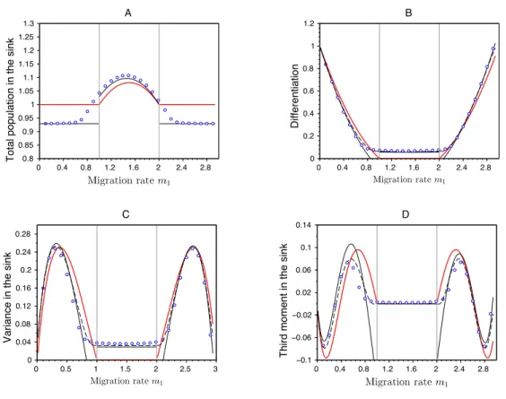
s1). In habitat 2, the evolutionary outcome results from the balance between migration from habitat 1 and local selection. Interestingly, migration has a non-monotonic e↵ect on adaptation in the sink (See Figure 6). Indeed, Figure 6A shows that the population size in the sink is maximized for interme-diate values of migration. More migration from the source has a beneficial e↵ect on the demography of the sink but it prevents local adaptation. Yet, when migration from the source becomes very large it limits the size of the population in the source (see (20)). This limits the influence of the source on the sink and can even promote adaptation to the sink. In fact, it is worth noting that di↵erentiation between the two habitats can actually increase with migration (Figure 6B). The level of migration from the source that prevents local adaptation in the sink is given by the condition:
4s2✓2rmax,2
2
m1(rmax,1 m1) 1
. (21)
Indeed, when condition (21) is verified, the migration from the source overwhelms local selection and the evolutionary stable strategy in the sink is z⇤ = ✓. In contrast, when condition (21) does not hold, the e↵ective growth rate of the optimal trait ✓ in the sink habitat is high enough to compete with the trait ✓ coming from the source, allowing coexistence between the two strategies. Note again that our two approximations (see supplementary information sections A.2.2.2 for the derivation of the first approximation and B.4 for the analytic formula for the moments of the phenotypic distribution derived from our second approximation) provide very good predictions for the moments of the phenotypic distribution in the sink (Figure 6).
4
Discussion
The balance between selection, migration and mutation drives the dynamics of local adaptation in heterogeneous environments. Here we present a new theoretical approach to obtain accurate approx-imations for the equilibrium phenotypic densities in a two-habitat environment. This analysis goes beyond the Adaptive Dynamics framework because it allows us to account for the e↵ect of large mutation rates. This analysis does not rely on the Gaussian approximation which underlies many Quantitative Genetics models. Our analysis yields analytic approximations that help provide a good understanding of the balance between the di↵erent evolutionary forces in both symmetric and non-symmetric scenarios.
In the symmetric scenario we recover the classical results from Quantitative Genetics in a single pop-ulation Lande 1975; B¨urger 2000; Rice 2004 but expand this to spatially heterogeneous scenarios. In particular, we capture the emergence of di↵erentiation between habitats when the migration rate decreases. When migration is strong relative to selection, the stationary phenotypic density is uni-modal in each habitat but heterogeneous selection increases phenotypic variance and di↵erentiation (see (19) and Figure 4). When migration is close to the critical migration rate mc (see condition (18)) we observe a shift between the phenotypic distributions of the two habitats. This pattern was not
0 0.4 0.8 1.2 1.6 2 2.4 2.8 0.8 0.85 0.9 0.95 1 1.05 1.1 1.15 1.2 1.25 1.3
Total population in the sink
A 0 0.4 0.8 1.2 1.6 2 2.4 2.8 0 0.2 0.4 0.6 0.8 1 1.2 Differentiation B 0 0.5 1 1.5 2 2.5 3 0 0.04 0.08 0.12 0.16 0.2 0.24 0.28
Variance in the sink
C 0 0.4 0.8 1.2 1.6 2 2.4 2.8 −0.1 −0.06 −0.02 0.02 0.06 0.1 0.14
Third moment in the sink
D
Figure 6 – E↵ects of migration in a source-sink scenario on (A) the total population size in the sink habitat, (B) the di↵erentiation between habitats, (C) the variance and (D) the third central moment of the phenotypic distribution in sink. The dots refer to exact numerical computations when " = 0.05, the red line indicates the case where " = 0 while the lines in black refer to our two approximations when " = 0.05 (dashed line for the first approximation and the full line for the second approximation). The vertical gray lines, at m1 = 1 and m1 = 2, indicate the critical migration rates where transition occurs between monomorphism and dimorphism in the Adaptive Dynamics framework (see condition (21)). Note that both approximations predict the same total population size. Other parameter values: rmax,1 = 3, rmax,2 = 1, s1 = 3, s2 = 2, 1 = 2 = 1, ✓ = 0.5, U = 1.
detected in previous studies but our method captures this shift and improves the approximation of the variance of the phenotypic distributions (see D´ebarre et al. 2013 and Figure 3). When the migration rate is much smaller than mc and selection is sufficiently strong between habitats, the equilibrium distribution in each habitat can be well approximated as the sum of two distributions. But unlike previous approximations Yeaman and Guillaume 2009; D´ebarre et al. 2013 these two distributions are non-gaussian. We derive approximations for the moments of these distributions. In other words, this work generalises previous attempts to derive the distribution of a phenotypic trait at the mutation-selection-migration equilibrium. Our results confirm the importance of the skewness in the phenotypic distribution and improve predictions of measures of local adaptation in a heterogeneous environment. In the non-symmetric scenario we show that the condition for the maintenance of two specialized
strategies are more restrictive (Figure 5). Indeed, asymmetries promote a single strategy that is more locally adapted to the habitat with larger population size and/or lower immigration rate. The impact of biased migration rates from a source population into the adaptation of peripheral populations has been discussed before Holt and Gaines 1992; Garc´ıa-Ramos and Kirkpatrick 1997; Gomulkiewicz et al. 1999; Holt et al. 2003; Akerman and B¨urger 2014. Our approach, however, yields a quantitative de-scription of the shape of the phenotypic distributions in both the source and the sink habitats. These accurate predictions are key to understand the e↵ect of di↵erent evolutionary forces on the level of adaptation in the two habitats. For instance, the analysis of an extreme case with source-sink dynamics reveals the complex interplay between migration, demography and local selection. The maintenance of a polymorphic equilibrium is possible when migration from the source is either very weak or very strong. This result challenges the classical prediction where migration is always an homogenizing force reducing the di↵erentiation among populations (Figure 6).
Our work illustrates the potential of a new mathematical tool in the field of evolutionary biology. In this work, we use an approach based on Hamilton-Jacobi equations (see (A.22)) which has been developed, mostly by the mathematical community, during the last decade to describe the asymptotic solutions of the selection-mutation models, as the e↵ect of mutation vanishes. We refer to Diekmann et al. 2005; Perthame and Barles 2008; Mirrahimi 2011 for the establishment of the basis of this ap-proach. Note, however, that previous studies were mainly focused on the limit case where the e↵ects of mutations are vanishingly small. In particular, they do not provide approximations of the phenotypic density and its moments when the e↵ect of mutations, ", is nonzero. In the present work we go further than the previous studies and characterize the phenotypic distributions when the influx of mutations can alter significantly the shape of the stationary distribution. Understanding the build up of this dis-tribution is particularly important to study the e↵ect of mutation on adaptation. Although mutation is the ultimate source of adaptive variation, the accumulation of deleterious mutations generates a load on the average fitness of populations. This is particularly relevant in organisms like RNA viruses which are characterized by very large mutation rates Drake and Holland 1999; Sanju´an et al. 2010. In fact, the mutation loads of RNA virus is so high that it may even lead some populations to extinction Bull et al. 2007; Martin and Gandon 2010. Our model can be used to accurately capture the e↵ect of increasing mutation rates on the mutation load of a population living in a heterogeneous environment (Figure 7). This heterogeneity may be particularly relevant in chronic infections by pathogenic virus that can adapt to di↵erent organs Kemal et al. 2003; Sanju´an et al. 2004; Ducoulombier et al. 2004; Jridi et al. 2006. A better understanding of the phenotypic distribution at equilibrium in heteroge-neous environments may thus provide more accurate prediction on the critical mutation rates that can ultimately lead within-host dynamics to pathogen extinction.
Our analysis of the equilibrium between selection, migration and mutation could be extended in several new directions. More than 2 habitats could be considered, or di↵erent growth rates and/or mutation kernels could be used (see Mirrahimi 2013 and the supplementary information, Section A.3). The approach could also be used to analyze situations away from the equilibrium. For instance, it would be possible to track the dynamics of the distribution as the population adapts to a new environment or to a time-varying environment Lande and Shannon 1996. Hamilton-Jacobi equations have indeed also been used to study time-varying (but space homogeneous) environments (see for instance Mir-rahimi et al. 2015; Figueroa Iglesias and MirMir-rahimi 2018). Finally, it is interesting to note that the generalization of the present ecological scenario to model the adaptation of sexual species in hetero-geneous environments remains to be carried out. Our method could be extended to allow for sexual
0 1 2 3 4 5 6 7 8 9 0 0.1 0.2 0.3 0.4 0.5 0.6 0.7
Total population size
Figure 7 – E↵ect of increasing the mutation rate U on the total population size in the symmetric scenario used in Figure 3 with m = 0.5. The full line indicates the approximation and the dots are the results of exact numerical computations. This figure illustrates that our approximation given by the first line of (19) captures reasonably well the e↵ect of large mutation rates on the mutation load in a two-habitat scenario where there is di↵erentiation and some local adaptation.
reproduction within the framework of the infinitesimal model (see Fisher 1919; Calvez et al. 2019). But this analysis falls beyond the scope of the present paper.
Acknowledgements
The first author is grateful for partial funding from the European Research Council (ERC) under the European Union’s Horizon 2020 research and innovation programme (grant agreement No 639638), held by Vincent Calvez, and from the french ANR projects KIBORD ANR-13-BS01-0004 and MOD-EVOL ANR-13-JS01-0009.
References
Akerman, A. and B¨urger, R. (2014). The consequences of gene flow for local adaptation and di↵eren-tiation: a two-locus two-deme model. Journal of Mathematical Biology, 68(5):1135–1198.
Barles, G., Mirrahimi, S., and Perthame, B. (2009). Concentration in Lotka-Volterra parabolic or integral equations: a general convergence result. Methods Appl. Anal., 16(3):321–340.
Bull, J. J., Sanjuan, R., and Wilke, C. O. (2007). Theory of lethal mutagenesis for viruses. Journal of virology, 81(6):2930–2939.
B¨urger, R. (2000). The Mathematical theory of selection, recombination and mutation. Wiley, New-York.
Calvez, V., Garnier, J. and Patout, F. (2019) A quantitative genetics model with sexual mode of reproduction in the regime of small variance. Preprint arXiv:1811.01779.
Caswell, H. (1989). Matrix Population Models. Sinauer Associates.
Champagnat, N., Ferri`ere, R., and M´el´eard, S. (2008). Individual-based probabilistic models of adaptive evolution and various scaling approximations, volume 59 of Progress in Probability, pages 75–114. Birkh¨auser.
Christiansen, F. B. (1975). Hard and soft selection in a subdivided population. The American Naturalist, 109(965):11–16.
Day, T. (2000). Competition and the e↵ect of spatial resource heterogeneity on evolutionary diversi-fication. The American Naturalist, 155(6):790–803.
D´ebarre, F. and Gandon, S. (2010). Evolution of specialization in a spatially continuous environment. Journal of Evolutionary Biology, 23(5):1090–1099.
D´ebarre, F., Ronce, O., and Gandon, S. (2013). Quantifying the e↵ects of migration and mutation on adaptation and demography in spatially heterogeneous environments. Journal of Evolutionary Biology, 26:1185–1202.
D´ebarre, F., Yeaman, S., and Guillaume, F. (2015). Evolution of quantitative traits under a migration-selection balance: when does skew matter? The American Naturalist, 186(37–47).
Diekmann, O., Jabin, P.-E., Mischler, S., and Perthame, B. (2005). The dynamics of adaptation: an illuminating example and a Hamilton-Jacobi approach. Th. Pop. Biol., 67(4):257–271.
Doebeli, M. and Dieckmann, U. (2003). Speciation along environmental gradients. Nature, 421:259– 264.
Drake, J. W. and Holland, J. (1999). Mutation rates among rna viruses. Proceedings of the National Academy of Sciences of the United States of America, 96(24):13910–3.
Ducoulombier, D., Roque-Afonso, A.-M., Di Liberto, G., Penin, F., Kara, R., Richard, Y., Dussaix, E., and F´eray, C. (2004). Frequent compartmentalization of hepatitis c virus variants in circulating b cells and monocytes. Hepatology, 39(3):817–825.
Fabre, C., M´el´eard, S., Porcher, E., Teplitsky, C., and A., R. (2012) Evolution of a structured population in a heterogeneous environment. Preprint.
Figueroa Iglesias, S. and Mirrahimi, S. (2018). Long time evolutionary dynamics of phenotypically structured populations in fluctuating environments. SIAM J. Math. Anal., 50(5):5537–5568. Fisher, R. A. (1919) Xv.-the correlation between relatives on the supposition of mendelian inheritance.
Gandon, S. and Mirrahimi, S. (2016) A Hamilton-Jacobi method to describe the evolutionary equilibria in heterogeneous environments and with nonvanishing e↵ects of mutations. Comptes Rendus -Mathematique, 355(2):155–160.
Garc´ıa-Ramos, G. and Kirkpatrick, M. (1997). Genetic models of adaptation and gene flow in periph-eral populations. Evolution, 51(1):21–28.
Geritz, S. A. H., Kisdi, E., M´eszena, G., and Metz, J. A. J. (1998). Evolutionarily singular strategies and the adaptive growth and branching of the evolutionary tree. Evol. Ecol, 12:35–57.
Gomulkiewicz, R., Holt, R. D., and Barfield, M. (1999). The e↵ects of density dependence and immigration on local adaptation and niche evolution in a black-hole sink environment. Theoretical population biology, 55(3):283–296.
Holt, R. D. and Gaines, M. S. (1992). Analysis of adaptation in heterogeneous landscapes: implications for the evolution of fundamental niches. Evolutionary Ecology, 6(5):433–447.
Holt, R. D., Gomulkiewicz, R., and Barfield, M. (2003). The phenomenology of niche evolution via quantitative traits in a ‘black-hole’ sink. Proceedings of the Royal Society of London B: Biological Sciences, 270(1511):215–224.
Jridi, C., Martin, J.-F., Marie-Jeanne, V., Labonne, G., and Blanc, S. (2006). Distinct viral popula-tions di↵erentiate and evolve independently in a single perennial host plant. Journal of Virology, 80(5):2349–2357.
Kemal, K. S., Foley, B., Burger, H., Anastos, K., Minko↵, H., Kitchen, C., Philpott, S. M., Gao, W., Robison, E., Holman, S., et al. (2003). Hiv-1 in genital tract and plasma of women: compart-mentalization of viral sequences, coreceptor usage, and glycosylation. Proceedings of the National Academy of Sciences, 100(22):12972–12977.
Kimura, M. (1965). A stochastic model concerning the maintenance of genetic variability in quanti-tative characters. Proc. Natl. Acad. Sci. USA, 54:731–736.
Kingman, J. F. C. (1978). A simple model for the balance between selection and mutation. J. Appl. Prob., 15:1–12.
Lande, R. (1975). The maintenance of genetic variability by mutation in a polygenic character with linked loci. Genetical Research, 26(3):221?235.
Lande, R. and Shannon, S. (1996). The role of genetic variation in adaptation and population persis-tence in a changing environment. Evolution, 50(1):434–437.
Leimar, O., Doebeli, M., and Dieckmann, U. (2008). Evolution of phenotypic clusters through com-petition and local adaptation along an environmental gradient. Evolution, 62(4):807–822.
Lenormand, T. (2002). Gene flow and the limits to natural selection. Trends Ecol Evol, 17(4):183–189. Martin, G. and Gandon, S. (2010). Lethal mutagenesis and evolutionary epidemiology. Philosophical
Transactions of the Royal Society of London B: Biological Sciences, 365(1548):1953–1963.
Mesz´ena, G., Czibula, I., and Geritz, S. (1997). Adaptive dynamics in a 2-patch environment: a toy model for allopatric and parapatric speciation. Journal of Biological Systems, 5(02):265–284.
Metz, J.A.J. and Nisbet , R. M. and Geritz, S. A. H. (1992) How should we define ’fitness’ for general ecological scenarios? Trends Ecol Evol , 7(6):198–202.
Mirrahimi, S. (2011). Concentration phenomena in PDEs from biology. PhD thesis, Univeristy of Pierre et Marie Curie (Paris 6).
Mirrahimi, S. (2013). Migration and adaptation of a population between patches. Discrete and Continuous Dynamical Systems - Series B (DCDS-B), 18(3):753–768.
Mirrahimi, S. (2017). A Hamilton-Jacobi approach to characterize the evolutionary equilibria in heterogeneous environments. Math. Models Methods Appl. Sci., 27(13):2425–2460.
Mirrahimi, S., Perthame, B., and Souganidis, P. E. (2015). Time fluctuations in a population model of adaptive dynamics. Annales de l’Institut Henri Poincare (C) Analyse Non Lin´eaire, 32(1):41–58. Nagylaki, T. (1978). A di↵usion model for geographically structured populations. Journal of
Mathe-matical Biology, 6(4):375–382.
Perthame, B. and Barles, G. (2008). Dirac concentrations in Lotka-Volterra parabolic PDEs. Indiana Univ. Math. J., 57(7):3275–3301.
Rice, S. H. (2004). Evolutionary theory: mathematical and conceptual foundations. Sinauer Associates, Inc.
Ronce, O. and Kirkpatrick, M. (2001). When sources become sinks: migration meltdown in heteroge-neous habitats. Evolution, 55(8):1520–1531.
Sanju´an, R., Codo˜ner, F. M., Moya, A., and Elena, S. F. (2004). Natural selection and the organ-specific di↵erentiation of hiv-1 v3 hypervariable region. Evolution, 58(6):1185–1194.
Sanju´an, R., Nebot, M., Chirico, N., Mansky, L., and Belshaw, R. (2010). Viral mutation rates. Journal of Virology, 84(19):9733–9748.
Savolainen, O., Lascoux, M., and Meril¨a, J. (2013). Ecological genomics of local adaptation. Nature Reviews Genetics, 14:807–820.
Slatkin, M. (1978). Spatial patterns in the distributions of polygenic characters. Journal of Theoretical Biology, 70(2):213 – 228.
Szil´agyi, A. and Mesz´ena, G. (2009). Two-patch model of spatial niche segregation. Evolutionary Ecology, 23(2):187–205.
Turelli, M. (1984). Heritable genetic variation via mutation-selection balance: Lerch’s zeta meets the abdominal bristle. Theoretical Population Biology, 25(2):138 – 193.
Whitlock, M. C. (2015). Modern approaches to local adaptation. The American Naturalist, 186(S1):S1– S4. PMID: 26098334.
Yeaman, S. and Guillaume, F. (2009). Predicting adaptation under migration load: the role of genetic skew. Evolution, 63(11):2926–2938.
Part
Supporting Information
Table of Contents
A
Mathematical derivation
2A.1 One population . . . 2
A.1.1 Derivation of our first approximation in absence of migration . . . . 2
A.1.2 Derivation of our second approximation in absence of migration . . 4
A.2 Two populations. . . 5
A.2.1 A general case (where m1 > 0 and m2 > 0) . . . 6
A.2.2 The extreme source and sink case (where m1 > 0 and m2 = 0) . . . 11
A.3 Derivation of a Hamilton-Jacobi equation in the case of model (2) . . . 15
B
Some expressions for the case studies
16B.1 Local densities in the dimorphic case for general and symmetric scenarios 16
B.2 Condition for dimorphism in a general non-symmetric scenario . . . 17
B.3 Analytic formula for the moments of the dimorphic phenotypic distribu-tion in the symmetric case . . . 17
A
Mathematical derivation
In this section, we provide the mathematical derivation of our results. In Section A.1 we treat the case of one habitat. In Section A.2 we provide our derivations for the case of two habitats. Finally in Section A.3 we show how our method can be used to study model (2).
A.1 One population
A.1.1 Derivation of our first approximation in absence of migration
Our first approximation is based on the computation of the terms u0(z) and v0(z). Based on such com-putations we can provide an approximation of the population’s total density N",0⇤ and the phenotypic density n⇤",0(z) in the following form
N",0⇤ ⇡ N0+ "K0, n⇤",0(z)⇡ 1 p 2⇡"exp u0(z) + "v0(z) " . (A.1)
Indeed we neglect the error term in (9) since when " is small, in view of (7), it has only small contribution to the phenotypic density n⇤",0(z).
We will prove in what follows that N0 = N0⇤, with N0⇤ the total population size at the demographic equilibrium of the ESS z0. We will also compute the other terms of the expansions K0, u0(z) and v0(z).
Using (5) and " =pVm, the equilibrium n⇤",0(z) solves: 0 = U "2@
2n⇤ ",0(z)
@z2 + n⇤",0(z) r0(z) 0N",0⇤ . (A.2) Replacing (7) in the above equation we obtain:
0 = U "@ 2u ",0(z) @z2 + U| @ @zu",0(z)| 2+ r 0(z) 0N",0⇤ . (A.3) This equation is derived using the following equalities:
@ @zn ⇤ ",0(z) = @ @zu",0(z) n⇤",0(z) " , @2 @z2n⇤",0(z) = ✓ "@ 2 @z2u",0(z) +| @ @zu",0(z)| 2 ◆n⇤ ",0(z) "2 . We then replace the ansatz (9) in (A.3). We first keep the zero order terms with respect to " (the ones in front of which there is no ", corresponding to the dominant terms) to obtain the following equation on u0(z):
0 = U|@zu0(z)|2+ r0(z) 0N0.
Note also that to have a finite but positive size of population, we should have max
z2R u0(z) = 0.
Otherwise, in view of (7), the total population size whether becomes infinite as "! 0 (if maxz2Ru0(z) > 0) or it goes to 0 (if maxz2Ru0(z) < 0).
At the maximum point zmaxof u0, we have @zu0(zmax) = 0 and hence r0(zmax) 0N0 = 0.
For all other traits z
r0(z) 0N0 = U|@zu0(z)|20.
We deduce that zmax is the maximum point of r0(z), that is zmax = z0. In other words, u takes its maximum at the ESS point z0 and the zero order term N0 in the approximation of the population size is given by
N0= r0(z0)
0
. (A.4)
This corresponds indeed to the total population size N0⇤ at the demographic equilibrium of the ESS z0. We gather our results on u0 in the following form Perthame and Barles 2008; Barles et al. 2009: u0 is indeed the unique solution to the following Hamilton-Jacobi equation
(
0 = U|@zu0(z)|2+ w(z; N0⇤), maxzu0(z) = u0(z0) = 0,
(A.5) where we recall that w(z; N0⇤) = r0(z) 0N0⇤. This equation can be solved explicitly. The solution u0(z) is given by u0(z) = 1 p U Z z z0 q
w(y, N0⇤)dy . (A.6)
The reader can verify that u0(z), given by the formula above, is smooth and solves (A.5). Note that the absolute values are necessary since the upper limit of the integral z can be smaller or larger than the lower limit z0.
We then keep the terms of order "
U @ 2 @z2u0(z) = 2U @ @zv0(z) @ @zu0(z) 0K0. (A.7)
An evaluation of this equation at the point z0 gives K0 =
U 0
@2
@z2u0(z0). (A.8)
The function v0(z) can also be computed thanks to (A.7), that is by integrating the following quantity @
@zv0(z) =
U@z@22u0(z) + 0K0 2U@z@u0(z)
. (A.9)
Note that to compute v0(z) we also need to choose the value of v0(z0). This value is fixed in a way
such that Z 1 1 1 p 2⇡"exp u0(z) + "v0(z) " dz = N ⇤ 0 + "K0. (A.10)
point of r0(z), is given by z0= ✓0. Considering the specific fitness function (10) in (A.4) we first obtain that
N0⇤= rmax,0 0
. Using (A.6) we then obtain that
u0(z) = p1 U Z z ✓0 p s0(y ✓0)2dy = ps 0 2pU(z ✓0) 2.
We also obtain from (A.8) that K0 = p
s0U
0 . Moreover, from (A.9) we obtain that @z@ v0(z) = 0 which means that v0(z) is a constant. Combining these informations with (A.10) we obtain
N",0⇤ ⇡ 1 0 (rmax,0 " p s0U ), n⇤",0(z)⇡ 1 p 2⇡"exp u0(z) + "v0(z) " = N",0⇤ s1/40 p 2⇡"pU exp ps 0 2"pU(z ✓0) 2 .
In other words, our first approximation of the phenotypic density n⇤",0(z) is given by (8) and (11). We note finally that the Gaussian distribution obtained above solves (A.2) and hence it is indeed an exact solution.
Example of non-symmetric growth rate (12). In this example similarly to the previous example the ESS z0 is given by z0= ✓0 and
N0⇤= rmax,0 0
.
The expression of u0(z) is however di↵erent, and it is given thanks to (A.6) by u0(z) = 1 p U Z z ✓0 p s0(y ✓0)2(a + (y ✓0 b)2)dy . (A.11)
From this expression we can then compute K0 and v0(z) similarly to above using (A.8) and (A.9).
A.1.2 Derivation of our second approximation in absence of migration
In this section, we provide the main idea to obtain explicit formula for the moments of the population’s distribution. The computation of explicit formula for the moments of the population’s distribution is based on the observation that, when " is small, the phenotypic density n⇤",0(z) is exponentially small far from the ESS point, since u0(z) takes negative values at those points. Therefore, only the values of u0(z) and v0(z) around the ESS point matter. We indeed use the Taylor expansions of u0(z) and v0(z) around the ESS point to compute such analytic formula.
We first provide our analytic formula for the moments of the population’s distribution. We next show how to compute such approximations.
Analytic formula for the moments of the population’s distribution. According to Section 3.1.1 there exists a unique ESS which is monomorphic and given by z0. In order to provide an explicit approximation of the moments of the population’s distribution, we compute the third order approximation of u0(z) around z0: u0(z) = A 2(z z0) 2+ B(z z 0)3+ O(z z0)4, (A.12)
and the first order approximation of v0(z) around z0: v0(z) = log(
p
AN0⇤) + D(z z0) + O(z z0)2. (A.13)
Such coefficients can be computed thanks to (A.6) and (A.9). To obtain the zero order term in the expansion for v0(z) we use the fact that, as the mutation’s variance vanishes (" ! 0), the total population size N",0⇤ tends to N0⇤ which corresponds to the demographic equilibrium at the ESS. The above approximation allows us to estimate the moments of the population’s distribution:
8 > > < > > : µ⇤",0= N1⇤ ",0 R zn⇤",0(z)dz = z0+ "(3BA2 +DA) + O("2), ⇤ 2 ",0= N1⇤ ",0 R (z µ⇤",0)2n⇤ ",0(z)dz = A" + O("2), ⇤ ",0= N1",0⇤ R (z µ⇤",0)3n⇤",0(z)dz = 6BA3"2+ O("3). (A.14)
Derivation of the analytic formula. We next show how to compute such approximations. We can indeed use the expressions in (A.12) and (A.13) to compute for any integer k 1,
R (z z0)kn⇤",0(z)dz = "k2pAN⇤ 0 p 2⇡ R R(yke A
2y2 1 +p"(By3+ Dy) + O(") dy = "k2N⇤ 0 ⇣ !k(A1) +p" B!k+3(A1) + D!k+1(A1) ⌘ + O("k+22 ),
where !k( 2) corresponds to the k-th order central moment of a Gaussian distribution with vari-ance 2. Note that to compute the integral terms above we have performed a change of variable z z0 =p"y, therefore each term z z0 can be considered as of order p" in the integrations. Note also that since the term v is multiplied by " in (9), a first order expansion of v is enough, while a third order expansion of u is required to obtain the above approximation. The above integrations are the main ingredients to obtain the approximations given in (A.14), i.e. our second approximation.
Example of non-symmetric growth rate (12). Using (A.11) and (A.9) we can compute the coefficients in the Taylor expansions of u0(z) and v0(z), that is (A.12) and (A.13), to obtain
A = p s0(a + b2) p U , B = ps 0b 3pU (a + b2), D = b a + b2.
Then the expressions of µ⇤",0, ⇤2",0and ",0⇤ at the end of Section 3.1.2 can be derived thanks to (A.14).
A.2 Two populations
This section is devoted to the mathematical derivation of our results in the case of two habitats. In Subsection A.2.1 we provide the mathematical derivation of our result in the general case. In Subsec-tion A.2.2 we treat the extreme case where there is no migraSubsec-tion from habitat 2, that is m2 = 0.
A.2.1 A general case (where m1 > 0 and m2 > 0)
In Subsection A.2.1.1, we provide the details of our results in the Adaptive Dynamics framework. In Subsection A.2.1.2 we present the analysis to obtain our first approximation. In Subsection A.2.1.3 we provide the derivation of our second approximation.
A.2.1.1 Adaptive dynamics in presence of migration In this section, we provide the
con-ditions for a global evolutionary stable strategy. To be able to characterize the ESS one should first characterize the demographic equilibrium corresponding to a set of traits. Because there are only two habitats, at most two distinct traits can co-exist. Therefore, we only need to consider two scenarios where the phenotypic distribution is either monomorphic (with phenotype zM) or dimorphic (with phenotypes zID and zIID, where the subscripts I and II indicate that the phenotype is best adapted to habitat 1 and 2, respectively).
The monomorphic equilibrium is given by nM
i (z) = NiM (z zM) where (.) is the dirac delta function, N1M, N2M T is the right eigenvector associated with the dominant eigenvalue W (zM; N1M, N2M) = 0 of A(zM; NM
1 , N2M). In a similar way the dimorphic equilibrium is characterized by: nDi (z) = ⌫I,i (z zID) + ⌫II,i (z zDII), where ⌫I,i + ⌫II,i = NiD and (⌫k,1, ⌫k,2)T are the right eigenvectors associated with the largest eigenvalues W (zDk; N1D, N2D) = 0 (for k = I, II) ofA(zkD; N1D, N2D).
The evolutionary stability of a resident strategy zM⇤ can be studied with the analysis of the invasion of a new mutant strategy zm at the demographic equilibrium N1M⇤, N2M⇤ set by the resident strat-egy. The monomorphic strategy zM⇤ is an evolutionary stable strategy if for any mutant zm 6= zM⇤, the e↵ective fitness is negative: W (zm; N1M⇤, N2M⇤) < 0. In a similar way, the dimorphic strategy {zID⇤, zIID⇤} is an evolutionary stable strategy if for any mutant zm 62 {zID⇤, zD⇤II }, the e↵ective fitness is negative: W (zm; N1D⇤, N2D⇤) < 0.
To determine the global ESS, we first define zD⇤ = r ✓2 m1m2 4✓2s 1s2 , N1D⇤ = m1m2 4✓2s2 + rmax,1 m1 1 , N2D⇤ = m1m2 4✓2s1 + rmax,2 m2 2 . Theorem A.1 Mirrahimi 2017 There exists a unique global ESS.
(i) The ESS is dimorphic if
m1m2 4s1s2✓4 < 1, (A.15) 0 < m2N2D⇤+ (w1( zD⇤; N1D⇤) m1)N1D⇤, (A.16) and 0 < m1N1D⇤+ (w2(zD⇤; N2D⇤) m2)N2D⇤. (A.17)
Then the dimorphic equilibrium is given by
nD⇤i = ⌫I,i (z + zD⇤) + ⌫II,i (z zD⇤), ⌫I,i+ ⌫II,i= NiD⇤, i = 1, 2, with ⌫k,i given in Section B.1.
(ii) If the above conditions are not satisfied then the ESS is monomorphic. In the case where condition (A.15) is verified but the r.h.s. of (A.16) (respectively (A.17)) is negative, the fittest trait belongs to