3-dimensional surface imaging using Active Wavefront Sampling

3-Dimensional Surface Imaging Using Active Wavefront Sampling

by

Federico Frigerio

B.S.E., Mechanical and Aerospace Engineering (1995)

Princeton University

M.S., Mechanical Engineering (1997)

Massachusetts Institute of Technology

SUBMITTED TO THE DEPARTMENT OF MECHANICAL ENGINEERING IN PARTIAL FULFILLMENT OF THE REQUIREMENTS FOR THE DEGREE OF

DOCTOR OF PHILOSOPHY IN MECHANICAL ENGINEERING AT THE

MASSACHUSETTS INSTITUTE OF TECHNOLOGY JANUARY 2006

MASSACHUSETTS INSiTFTE

0 2006 Massachusetts Institute of Technology OF TECHNOLOGY

All rights reserved

JAN

0

2 2007

LIBRARIES

Signature of Author... ...

epartmen f Mechafical Engineering

January

C ertified by ... ...

Douglas P. Hart Professor of Mechanical Engineering Thesis Supervisor

'A

A ccep ted b y ... ,... ...

Lallit Anand Professor of Mechanical Engineering Chairman, Department Committee on Graduate Students

MIT Libraries

Document Services

DISCLAIMER OF QUALITY

Due to the condition of the original material, there are unavoidable

flaws in this reproduction. We have made every effort possible to

provide you with the best copy available. If you are dissatisfied with

this product and find it unusable, please contact Document Services as

soon as possible.

Thank you.

The images contained in this document are of

the best quality available.

3-Dimensional Surface Imaging Using Active Wavefront Sampling

by

Federico Frigerio

Submitted to the Department of Mechanical Engineering on January 1 9h, 2006 in Partial Fulfillment of the Requirements for the Degree of Doctor of Philosophy in

Mechanical Engineering

ABSTRACT

A novel 3D surface imaging technique using Active Wavefront Sampling (AWS) is presented. In

this technique, the optical wavefront traversing a lens is sampled at two or more off-axis locations and the resulting motion of each target feature is measured. This target feature image motion can be used to calculate the feature's distance to the camera. One advantage of this approach over traditional stereo techniques is that only one optical train and one sensor can be used to obtain depth information, thereby reducing the bulk and the potential cost of the equipment. AWS based systems are also flexible operationally in that the number of sampling positions can be increased or decreased to respectively raise the accuracy or to raise the processing speed of the system. Potential applications include general machine vision tasks, 3D endoscopy, and microscopy. The fundamental depth sensitivity of an AWS based system will be discussed, and practical implementations of the approach will be described. Algorithms developed to track target features in the images captured at different aperture sampling positions will be discussed, and a method for calibrating an AWS based method will also be described.

Thesis Supervisor: Douglas P. Hart

Contents

1

1.1 M otivation/B ackground ... 7

1.2 Introduction to Active Wavefront Sampling ... 12

1.3 Performance Potential of Active Wavefront Sampling ... 20

1.4 Roadmap for In-Depth Analysis of AWS-based 3D Imaging ... 26

2 Design and Implementation of AWS 27 2.1 Size of Sampling Aperture ... 27

2.2 Placement of Sampling Plane ... 28

2.3 Mechanical Implementation of AWS ... 30

2.4 Electronic Implementation of AWS ... 33

2.5 Illum ination of T arget ... 34

2.6 Implementation Using 50mm Nikkor Lens ... 36

3 Image Processing 41 3 .1 In troduction ... 4 1 3.2 Review of Motion Tracking Algorithms ... 41

3.3 Algorithms Developed for Two Image AWS Processing ... 58

3.4 Extension of Two-Image Algorithms to Many Sampling Locations ... 70

3.5 Multi-Image Algorithm Using Large Spatio-Temporal Filters ... 76

4 Calibration and Quantitative Measurement 91 4 .1 In troduction ... 9 1 4.2 Geometrical Optics Aberration Theory ... 93

4.3 Determination of Aberration Coefficients ... 100

4.4 Performance of Calibration Model ... 111

4.5 Comparison of Calibration Model to Linear Interpolation Method ... 117

5 Conclusions 5.1 Theoretical Background and Utility ... 123

5.2 Implementation of Active Wavefront Sampling ... 123

5.3 Motion Tracking Algorithms ... 124

Chapter 1: Introduction

1.1 Motivation/Background

For the past 150 years or so, one of the most efficient means to convey information about the world we live in has been through the use of two dimensional images. These images have been recorded and displayed using chemical or more recently with electronic techniques, and have been very effective at capturing and conveying the light intensity, color, and x and y coordinates of targets within a scene. Since these images record the two dimensional projection of our 3D world onto an imaging plane, all quantitative depth information is lost. Only subtle cues such as shading and the mind's a-priori knowledge of the scene allow the human observer to qualitatively extract depth cues from these two dimensional projections. Clearly, even these qualitative depth cues can fail the observer in situations where the target is completely unknown, or if depth ambiguities in the 2D projection exist which can easily fool the human observer. One such "optical illusion" is shown in Figure 1.1.

Because of the inherent limitations of 2D technology, making the transition from 2D to 3D image capture and display is extremely desirable. In terms of 3D capture, any endeavor requiring the quantitative measurement of a target's dimensions would benefit from a sensor system that could also measure depth. Some obvious applications include quality control of parts on an assembly line, facial recognition for security, autonomous vehicle navigation, measurement and registration of tissues during medical procedures, and 3D model capture for the movie and entertainment industries. Indeed, it is difficult to imagine any imaging application where the added capability to measure a target's depth along with its color, intensity, and its x and y position would not be welcome.

Figure 1.1 M.C. Escher Waterfall, 1961. An example of an optical illusion, where the clever use of shading and perspective are used to confuse the observer's visual system.

In terms of transitioning to 3D display technologies, only the latter can take advantage of the human user's "built in" stereoscopic vision system to further enhance the sensation of depth. Just as the use of fully rendered and shaded 2D projection graphics was a huge improvement over the previous use of point clouds, wireframe drawings or flat color projections, the jump to full fledged 3D display represents a huge improvement in how the user can perceive and manipulate target information. Indeed, the final addition of the stereoscopic depth cue should allow for the creation of near perfect virtual optical input; so perfect that the user has difficulty in differentiating between a real scene and its recorded version.

In order to overcome the inherent limitations of standard 2D imaging techniques, research into technologies that can capture and display the full three dimensional information in a scene has been very active. A survey of current technology suggests that image recording and display technology is in a transition stage from two dimensional to three dimensional techniques. In the case of 3D recording techniques, one of the oldest approaches to capturing depth information has been through the use of a pair of 2D recording devices whose relative orientation is known. Much like the optical system of predator animals in Nature, this depth from stereo approach is a triangulation technique that relies on the difference or disparity between the recorded position of

each target point on the two imaging sensors. For each target feature, the magnitude of this disparity is directly related to that feature's distance from the imaging system. Some of this technique's shortcomings include occlusion (where a target feature is visible to one sensor but not to the other), the need to constantly calibrate the system due to camera alignment difficulties, high cost due to the use of multiple camera/lens systems, and high computational cost due to large target feature disparities between one sensor and the other.

Laser scanning systems represent another approach that utilizes triangulation in order to capture the depth information in a scene. In a typical system, a laser sheet is swept across the target object and the position of the resultant line (which is the laser sheet's projection onto the target surface) is recorded by a camera. Just like in stereo camera systems, the relative position and orientation of the recording camera and the laser projector are known, so that the calculation of the laser line's position uniquely determines the distance from the sensor of target features along that line. Though laser scanners are amongst the most accurate 3D imaging systems available, some of this technique's inherent shortcomings include high cost, size and complexity, and scanning times on the order of seconds or minutes.

Figure 1.2. A typical laser scanner system, this Cyberware Model 3030 RGB/MS uses two linear and one rotational stages to capture full view 3D data from a target. Sampling pitch is 0.25-1.0mm in X and Y directions, and 50-200 microns in the Z direction. The translation table is approximately waist high.

Time of flight range scanners, meanwhile, measure the time taken by a pulsed laser beam to bounce off a target and return to its source. These systems are often used in surveying applications as their operating range reaches up to 100 meters. Their positional accuracy is typically about 6mm at 50 m distances, but their disadvantages include their complexity and expense, as well as prolonged operation time required to scan a full target scene.

Figure 1.3. Leica model HDS3000 time of flight range scanner. Mounted on a tripod at a worksite, this range scanner pulses a laser beam and measures the time taken by the beam to bounce off the target and return to its source. Typical accuracies are on the order of 6mm over target distances of 50 m.

Much progress has also been made in the development of devices that can use and display 3D data. For decades, computer graphics libraries have existed that allow the display and manipulation of shaded, photo realistic 2D projections of 3D objects on standard 2D displays. The ability to handle 3D data and display realistic 2D projections of that data has been useful in fields ranging from computer aided design (CAD) to entertainment applications like movies and video games. More recently, devices that seek to give the user an actual sensation of the target's depth (as opposed to just displaying the 2D projection of a 3D object) have become more common in the marketplace. For example, wearable display glasses that transmit the left and

right stereoscopic views to the user's corresponding eyes have been in use for some time and are quite good at creating a virtual reality effect. Computer screens with modified LCD screens are also appearing in the marketplace with some success. These create the impression of depth by having part of the LCD screen project the left image so that it is only visible to the user's left eye, and by having the other part of the LCD screen project the right image so that it is only visible to the user's right eye. Holography based technologies are also being developed that allow multiple users to achieve the same depth sensations from differing vantage points. A similar effect can also be obtained by projecting different 2D views of the 3D data on a rapidly rotating screen.

(a)

(b)

Figure 1.4. (a) Dimensions Technologies Inc. switchable 2D1/3D LCD monitor. A special illumination scheme behind the LCD panel

sends alternate pixel columns to the viewer's right and left eye, creating the stereoscopic illusion of depth without the user having to wear any special glasses. (b) Actuality Systems Perspecta Spatial 3D display uses a rotating screen onto which are projected different

It can be argued that at the current time, technologies to manipulate and display 3D datasets (either in full 3D fashion or simply through 2D display of photorealistic projections) are more widely diffused than 3D recording devices. This gap between 3D input and output technologies will need to be filled by improvements in current measurement devices, as well as by the development of entirely new approaches to the problem. One such approach may well be 3D surface imaging using active wavefront sampling, and the remainder of this thesis will attempt to describe it and to measure its capabilities.

1.2 Introduction to Active Wavefront Sampling

The active wavefront sampling (AWS) approach to 3D surface imaging has several attractive attributes. Its most important characteristic is that, unlike stereoscopic systems, it requires only one optical path to capture depth information. This attribute reduces system costs by halving the cost of the optics, and also allows the technique to be applied to a wide range of currently available 2D imaging systems such as cameras, endoscopes, and microscopes. AWS also reduces system cost by dispensing with expensive laser based target illuminators, and minimizes target acquisition time by not having to slowly sweep an illumination sheet across the target. Instead, the AWS approach can calculate a 3D depth map with as little as two image frames (like a stereo system), thereby allowing real time (>30 Hz) operation.

1.2.1 Depth-From-Defocus

In order to understand the fundamental principle behind the use of AWS to calculate depth, one must first analyze how a target feature's depth is encoded by the diameter of its defocus blur on the sensor plane. This principle is well known and is the basis for an entire range of 3D surface imaging techniques known as depth-from-defocus. As can be seen in Figure 1.5, the diameter of a target feature's defocus blur is directly related to that feature's distance from the optical

Fo

t-of-focus Focal Plane nt

.~ .... . .... .--. . ... - . .... . ... . . - . ... _ d

CCD Plane

Figure 1.5. Schematic of depth-from-defocus approach. In top diagram, the target feature of interest is located on the lens in-focus plane. The feature's image is perfectly in focus and its blur spot diameter is effectively zero. In the bottom diagram, the target feature of

interest is located some distance from the lens in-focus plane. The feature's image is out of focus, and the non-zero diameter of its blur spot is directly related to how far away the target is from the in-focus plane.

cal Plane

CCD PI

OU

Poi

system's in-focus plane. If the feature is situated on the in-focus plane, the target is in perfect focus and the defocus blur diameter is zero (neglecting diffraction effects). As the target feature moves away from the in-focus plane, however, the diameter of the defocus blur increases. A straightforward geometrical optics analysis of the system reveals that the image plane blur diameter can be calculated using the following expression:

d Y Z,

D

(1.1)

In equation 1.1, d is the disparity at the image plane in pixels, D is the diameter of the lens exit pupil,f is the focal length of the lens, Z, is the distance of the target to the lens, and Zfp is the distance of the in-focus plane to the lens' principle plane. Remembering that the denominator in Equation 1.1 is nothing but the distance of the lens' principle plane to the imaging sensor, ZCCD I the expression can be rewritten as follows:

d I

- =ZCC x - -

-D CCDZ,

Zz

(1.2)

When this expression is evaluated over a range of normalized target depths, the plot in Figure 1.6 is obtained. As expected, this plot shows that the blur diameter drops to zero when the target is located on the in-focus plane and that the blur diameter rises as the target moves away from the in-focus plane. It should be noticed that the sensitivity or accuracy of this method is directly proportional to the slope of the line in Figure 1.6, since a larger slope implies a greater disparity

change on the image plane (which is what is being measured) for a given change in target depth (which is what is being calculated).

d

Z/ Z P

Figure 1.6. Normalized blur spot diameter vs. normalized target distance to the principal plane. "d" is the blur spot diameter, "D" is the diameter of the lens exit pupil, "Zt" is the target distance to the principal plane, and "Zfp" is the distance of the focal plane to the principal plane.

In a typical depth-from-defocus system, the optical train's entire wavefront is allowed to travel through and hit the imaging plane. The challenge is then to calculate the diameter of each target feature's blur spot in order to determine its depth. The difficulty of accurately calculating the blur spot diameter and complications related to having overlapping blur spots from feature rich targets have traditionally limited the utility of depth-from-defocus techniques.

1.2.2 Static Wavefront Sampling

Certain limitations in standard depth-from-defocus techniques can be overcome by switching to a wavefront sampling approach. Unlike depth-from-defocus systems, the wavefront sampling approach only allows specific parts of the optical train's wavefront to reach the imaging plane.

The simplest sampling pattern that allows the calculation of a target feature's depth is a sampling plane with two apertures, as shown in Figure 1.7. This static wavefront sampling results in the formation of two quasi-in-focus images of the target feature. If the two static apertures are

separated by a distance equal in magnitude to the full exit pupil diameter of the depth-from-defocus case shown in Figure 1.6, then the separation between the two quasi-in-focus images resulting from the static wavefront sampling will be exactly equal to the blur spot diameter resulting from the depth-from-defocus approach (for the same optical train and target position conditions). In effect, one can think of wavefront sampling in terms of sampling the defocus blur. With a two aperture static wavefront sampling mask, the separation between the two images of the same target feature needs to be calculated in order to determine that feature's depth (determined by equation 1.1). There exist several motion tracking algorithms available, ranging from block matching methods (autocorrelation, etc...), optical flow techniques, and Fourier domain algorithms that can be used to determine this separation distance to within a small fraction of a pixel. However, the fact that multiple images of the same feature are recorded on each frame can still cause overlap problems when the target is feature rich and can also result in a depth ambiguity. Indeed, looking once again at Figure 1.6 shows that for a given disparity measurement, there are two possible target positions. One possible target position is located between the lens and the in-focus plane, and the other possible target position is located beyond the in-focus plane. Without any a priori knowledge of the target's position, it is impossible to tell from a double exposed image resulting from a static mask which of these two possible target positions is correct.

Sampling Position 1

Out-of-focus Focal Plane

CCD Plane

Sampling Position 2

Figure 1.7. Static sampling of the wavefront with two diametrically opposed apertures separated by a distance equal to the overall aperture diameter in Figure xx. Instead of a defocus blur of diameter d, two quasi-focused images separated by the same distance d are recorded on the image plane.

One implementation of a two aperture static sampling system has been carried out by researchers at the National Research Council of Canada (Blais and Rioux [1], and Beraldin et. Al. [2]). The BIRIS sensor comes in various versions but essentially consists of a camera and lens equipped with a two aperture mask, as well as a laser that projects a sheet onto the target (see Figure 1.8). Because of the two apertures, the laser line produces two images on the sensor plane and the depth of the target points illuminated by the laser is calculated by measuring the distance between the two image lines. The target depth is then calculated using equation 1.1. Just like with a regular laser scanner, this system needs to gradually scan the laser line across the target in order to obtain the entire depth map. Recent versions of the BIRIS system also takes advantage of triangulation between the camera and the laser projector to get a second estimate of the depth, and the final output is the result of taking a weighted average of the wavefront sampling derived depth

and of the triangulation derived depth. Because of this, the BIRIS system can be considered to be a hybrid approach between a laser scanning system and a true wavefront sampling system.

Laser

Z ---

---Object Ln

Mask .

Figure 1.8. Schematic of and typical image obtained from BIRIS range finding system. A two aperture mask is used to get an initial depth estimate, and triangulation between the laser projector and the camera is then used to obtain a higher accuracy depth estimate. On the right, a square pyramid (top) is illuminated with several laser light stripes and the resulting image with the lines doubled due to the two aperture mask is shown below. The distance between the two lines on the image is proportional to the depth of that part of the target.

By simple extension, more than two sampling positions can be used to estimate depth. A

sampling mask with three or more apertures would result in pictures with a corresponding number of target images. Measurements of the displacement between the various images of each target feature can be used to back calculate the actual depth of that feature. The exact transformation from the image displacement measurement to actual depth will depend on the pattern of the sampling mask, but is generated in a similar fashion as equation 1.1. Clearly, a higher potential depth estimation accuracy is attained with a greater number of sampling positions but at the same time a greater confusion is caused due to multiple image overlap with a feature rich target.

1.2.3 Active Wavefront Sampling

As was shown above, sampling the wavefront of an optical system with several apertures allows one to estimate the depth of a target feature. However, the use of static aperture masks results in a depth ambiguity (one cannot determine whether the target is located in front of or behind the in-focus plane) and can lead to confusion due to overlapping images from feature rich targets. One

solution to both problems is to use an active wavefront sampling approach. With this technique, a single aperture is moved from one position to another in the sampling plane and a single image is recorded at each spot. This results in clear single exposure images of the target with no confusion due to multiple image overlap, and the depth ambiguity present with a static mask is resolved so long as the motion of the aperture on the sampling plane is known. If, for example, a single aperture is rotated in a circle centered on the optical axis of the lens and images are taken at regular angular intervals, a movie of the resulting images would show the target also rotating in a circular pattern. Under these operating conditions, the depth information for each target feature is coded by the diameter of its rotation; a feature located right on the in-focus plane would have a zero diameter rotation (and would appear stationary) while features located at increasing distances from the focal plane would rotate along circles of greater and greater diameter. Furthermore, a target feature located beyond the in-focus plane will rotate 180 degrees out of phase with a target feature located between the lens and the in-focus plane. This phase difference therefore allows the resolution of the depth ambiguity present in depth-from-defocus and static aperture mask systems described earlier.

Of course, a circular pattern of aperture motion is not the only possible path that can be used with

AWS. The aperture can be simply translated in a horizontal, vertical, or diagonal line; or the aperture path can be chosen to follow any arbitrary closed loop. As long as the aperture path is known, target depth can in theory be recovered by tracking the resulting motion of each target feature from one image to the next. However, a simple circular aperture motion does have at least two major attractive qualities: the first is that it is relatively simple to implement

mechanically, and second is that it presents certain advantages for the processing algorithms used to track target features from one image to the next. These advantages will be discussed in more depth in Chapter 3.

Besides resolving the discussed depth ambiguity and the multiple image overlap problem, the active wavefront sampling approach allows the user to select from a wide range of operating regimes within the high accuracy/low speed - low accuracy/high speed domain. Indeed, for high speed imaging applications where some measurement accuracy can be sacrificed, as little as two wavefront sampling positions can be used to estimate a target feature's diameter of rotation. In this scenario, the displacement between the two images is taken as the estimate of the rotation diameter. For applications where higher accuracy is required but acquisition speed can be

sacrificed, more sampling positions can be used. In this multiple sampling position scenario, a circle can be fitted in the least square sense to the image positions, and the accuracy of the depth estimate will rise with the number of sampling positions.

1.3 Performance Potential of Active Wavefront Sampling

1.3.1 Depth Sensitivity of A WS-based System

As was discussed above, the idealized optical performance characteristics of the active wavefront sampling (AWS) approach are identical to those of the classic depth-from-defocus approach, as described quantitatively by Figure 1.6. Again, this figure shows that as a target feature moves farther away from the in-focus plane, the motion diameter of its image rotation caused by a circular aperture sampling pattern increases. This diameter increases more steeply if the target feature moves toward the lens than away from the lens. Also, it can be seen that if the target feature is moved away from the lens, the diameter asymptotically reaches a constant value. These characteristics suggest that the optimal operating regime for AWS based systems is defined by having the target located between the in-focus plane and the lens, where system sensitivity to depth is highest. This sensitivity can be calculated by taking the derivative of equation 1.2 with respect to target depth, and rearranging slightly:

di 1 = -D x _{ZCCD X}

(1.3)

All other things being equal, the field of view of the optical system decreases as the target is

brought closer to the lens. It is therefore instructive to generate a disparity sensitivity expression where the size of the field of view (in pixels, say) is kept constant by changing the distance between the lens and the sensor, ZCCD. In practice, this can be achieved by changing the focal length of the lens as the target is moved. By using similar triangles, it can be found that

Z

SFOV

(1.4)

where SSensor is the size of the CCD sensor, and SFOV is the size of the field of view (in pixels, say). Inserting equation 1.4 into equation 1.3 results in the following expression:

- -Dx Sensor

1

JZt SFOV Z,

(1.5)

With constant values for Ssensor and SFOV , it can be seen that the sensitivity of the AWS system

now varies inversely with Z,, as opposed to inversely with Z,2 in the case where the lens focal length is held constant and the field of view size is allowed to vary. The expressions in equations 1.4 and 1.5 are plotted in Figure 1.9 below, where it can be seen that the sensitivity of an AWS system drops off quickly with depth. Furthermore, it can also be seen from this figure that the depth sensitivity of a constant focal length AWS system drops off more quickly than the

0.03

--- _{Constant FOV}

Constant Focal Length

0.025-0.02 0.015 Co 0.01 0.005 0 0.5 1 1.5 2 2.5 3

Target Distance (pixels) _{x 10,}

Figure 1.9. Disparity gradient, cM , as a function of target distance, Zt .These simulations assumes a sampling diameter, D, of

800 pixels and a sensor size of 1024 pixels. For the constant field of view (FOV) size simulation, a constant FOV size of 8333 pixels

is used. For the constant focal length simulation, a constant lens to sensor distance of 4166 pixels is used.

1.3.2 Comparison to Standard Stereo Imaging

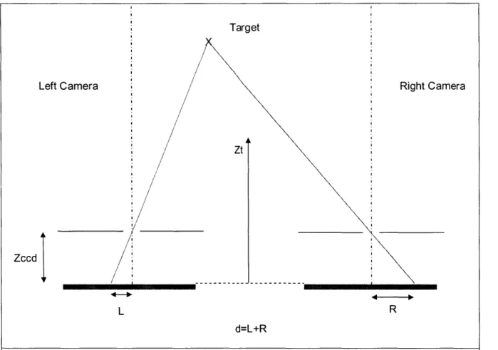
It is instructive to compare the performance of an AWS system to a standard depth-from-stereo imaging system (see Schechner and Kiryati [3], who compared a stereo system to a depth-from-defocus system). A canonical stereoscopic system has two cameras whose sensors are perfectly aligned (ie: they have parallel optical axes and aligned x axes), as can be seen in Figure 1.10. This schematic shows that a target feature produces an image at a different location on each image sensor.

Target Left Camera Zccd L / /

/

zt

d

1

Figure 1.10. Canonical stereo imaging system composed by a left and right camera. The distance from the optical axis of the target image on the left and right cameras is denoted by "L" and "R" respectively. The total disparity d is just the sum of these two distances.

The disparity between these images, d, is clearly related to the distance of the target to the cameras in the z direction. Indeed, a simple geometrical analysis reveals that the disparity between the two images is given by the following equation:

-= ZCCD

b

_Z,

(1.6)

In this equation, ZCCD is the distance from the lens' principal plane to the imaging sensor, b is the baseline distance between the optical axes of each camera, and Z, is the distance of the target

ht Camera

---they only differ by a constant term involving the distance of the in-focus plane to the camera lens. This fact can be seen in Figure 1.11, which shows the disparity between two images of a target feature for both the nominal stereo imaging system as well as the AWS imaging system.

600 C,, L Cn E

500

-100

0

-100,

0

0.5

Target Depth, Zt (pixels)

3

X 10

Figure 1.11. Disparity as a function of target depth (both in pixels) for an AWS system and for a canonical stereo system. Using the same values baseline/sampling diameter and lens-to-sensor distance, it can be seen that the two curves are identical but displaced by a constant amount. This constant is introduced by the l/Zfp term in equation 1.2.

Just like in the AWS case, the sensitivity to depth of the canonical stereo system can be estimated

by taking the derivative of equation 1.6 with respect to target distance. The following equation is

the result of this operation:

il

=

Comparing the above expression to equation 1.3, we see that the sensitivity to depth of a canonical stereo system and of an AWS system is exactly the same. It can therefore be concluded that an AWS system with two diametrically opposed sampling positions responds exactly like a

stereo system whose baseline is equal to the AWS sampling diameter. Therefore, the only physical system parameters that can be varied to increase depth sensitivity are the sampling diameter (equivalent to the baseline in a stereo system) and the distance of the principal plane of the lens to the imaging sensor (ZCCD). Depth sensitivity increases with sampling diameter, but the latter is limited by the lens' exit pupil size; the bigger the lens, the larger the maximum sampling diameter. Depth sensitivity also increases with ZCCD , but the field of view with a given lens also decreases as ZCCD is increased. Compromises must therefore be made in increasing lens size (and therefore increasing cost), and increasing ZCCD length (and decreasing

the field of view).

A typical commercial stereo system might be composed of two lenses and cameras separated by a

baseline on the order of 20cm, while an AWS system made with an identical lens and camera might only have a sampling diameter of 1 cm. All other things being equal, therefore, an AWS system using only two sampling positions would only have 1/2 0th the depth sensitivity of the stereo system. This difference in performance would at first seem to rule out the use of AWS in favor of a standard stereo system, but the comparison requires further examination. First of all, it must be remembered that the larger baseline present in stereo systems comes at the cost of greater occlusion (which is when a target feature is visible in one camera but not in the other), higher hardware cost, greater difficulty with calibration, and higher computational cost (since the matching problem needs to be solved over a larger disparity range). Additionally, there exist operating conditions where a large baseline is undesirable or completely impossible, such as with endoscopes used during surgical procedures; the diameter of the optical instrument in this case

certainly true that a stereo system may be on the order of 20 times more sensitive to depth than a similarly built AWS system that uses two sampling positions, this performance differential can be significantly reduced by increasing the number of sampling positions used by the AWS system. Indeed, it will be shown in later sections that the use of more than two sampling positions increases both the accuracy and the robustness of the algorithms that track target features from one image to another. The higher accuracy of these multi-sampling tracking algorithms results in a smaller uncertainty in the measurement of the target feature's rotation diameter. The better rotation diameter estimate therefore compensates for the shallower sensitivity curve caused by the smaller baseline present in AWS.

1.4 Roadmap for In-Depth Analysis of AWS-based 3D Imaging

With the brief introduction to the concept of using active wavefront sampling to calculate 3D surface models given in this first chapter, a detailed examination of the most important aspects of the approach can be discussed in the subsequent parts of this thesis. In Chapter 2, a description will be given of how the AWS concept can be implemented in hardware. This will include various approaches to moving a sampling aperture, as well as discussing the optimal placement of the sampling plane. Chapter 3 will concentrate on describing the algorithms required to track target features between images captured as the aperture is moved from one sampling position to the next. This third chapter will assume that the optical train behaves ideally, so that a circular motion of the sampling aperture leads to a circular motion of the target feature image on the image plane. In Chapter 4, this assumption will be removed and the effect of aberrations in the optical train will be incorporated. It will be shown that these aberrations can have a very important effect on the calculated target depth, even for relatively fast and expensive optical trains. Finally, Chapter 5 will summarize the results of this work and will indicate areas of potential future study.

Chapter 2: Design and Implementation of AWS

There are many possible ways to implement an AWS system, each with different hardware components and performance flexibility. The aperture sampling can be performed mechanically or electronically, and there are many different aperture sampling paths that can be used. Whether the sampling is implemented mechanically or electronically, the size of the aperture and the placement of the sampling plane itself should be optimized so as to maximize captured image quality. The target illumination method must also be considered as it can have a strong influence on image quality. These design parameters will now be discussed, and the simple mechanical setup used to obtain the results presented later on in this thesis will be described.

2.1 Size of Sampling Aperture

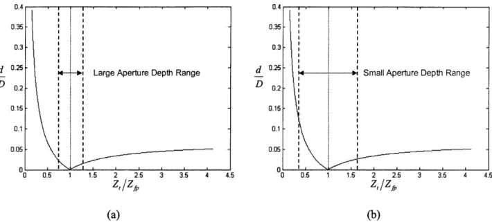
The size of the sampling aperture can have a strong effect on image quality. A larger aperture will be able to image higher frequency features due to its higher numerical aperture (NA), but it will also have a smaller depth of field which will reduce the depth range over which 3D surface imaging is possible to a narrower band surrounding the in-focus plane (see Figure 2.1 .a). A larger aperture will also allow for shorter image exposure times, thereby increasing the possible frame rate of the imaging system. Conversely, a smaller aperture size will increase the operable depth band (allowing increased depth sensitivities) but will low pass filter the image due to the smaller NA (see Figure 2.1 .b). The smaller aperture size will also require an increased exposure time, reducing the maximum frame rate of the system.

The aperture size representing the best tradeoff between depth range, spatial frequency sensitivity and frame rate will depend very much on the particular application at hand. However, we will see in Chapter 3 that the image processing algorithms used to track target features from one image to the next work best with low spatial frequency images, so that using a smaller aperture does not necessarily hinder the quality of the calculated 3D surface model.

0.4 0.4

0.35 - - 0.35

-0.3 -0.3

Large Aperture Depth Range 0.25 -- Small Aperture Depth Range

D 2D 0.15 I0.15 I 0.1 - 0.1 -0.05 - 0.05 I 0 0.5 1 1.5 2 2.5 3 3.5 4 4.5 0 0.5 1 1.5 2 2.5 3 3.5 4 4.5 Zt/ Z Z/ Z, (a) (b)

Figure 2.1. (a) Practical target depth range over which the AWS sampled image is in-focus enough to allow processing, for a large aperture size. (b) Practical target depth range over which the AWS sampled image is in-focus enough to allow processing, for a small aperture size.

2.2 Placement of the Sampling Plane

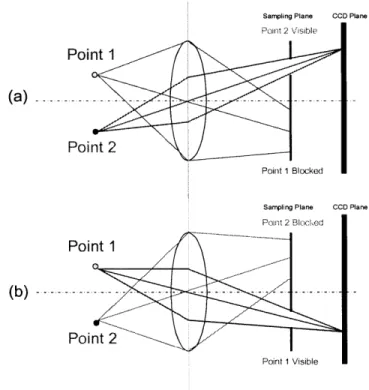
For a pre-existing optical system, the aperture sampling plane should be placed as close as possible to the optical train's exit pupil. This should be done so as to minimize vignetting and intensity variation as the aperture is moved from one sampling position to another. This effect can be seen in Figure 2.1 and Figure 2.2, where schematic ray traces of the image side of an optical system are drawn for the case of a sampling plane located far from the exit pupil and for the case of a sampling plane located right at the exit pupil, respectively. In Figure 2.1, the sampling plane is located at some distance from the optic's exit pupil. With the aperture in the top position, (Figure 2.1(a)), rays from point 2 are sampled while all rays from point 1 are blocked from reaching the sensor plane. Conversely, with the aperture in the bottom position (Figure 2.1(b)), rays from point 1 are sampled while all rays from point 2 are blocked. This vignetting condition is undesirable as target features cannot be tracked from one sampling position to the next resulting in a loss of 3D data. In contrast, Figure 2.2 shows the ray tracings for the case where the sampling plane is located right at the exit pupil. Here, we see that for both

Sampling Plane CCD Plane

Point 1

( a ) . ---- -- .... ...

....---Point 2

Point 1 Blocked

Sampling Plane CCD Plane

Point 2 Blc-cckod

Point 1

Point 2

Point 1 Visible

Figure 2.2. Effect of placing the sampling plane far from the exit pupil of the optical train. In case (a), the aperture is located at the top and light rays from Point 2 are able to reach the CCD plane while all light rays from Point 1 that pass through the lens are blocked. In case (b), the aperture is located at the bottom and all possible light rays from Point 2 are blocked while light rays from Point 1 are able to reach the CCD plane. This extreme vignetting prevents 3D surface reconstruction.

Sampling Plane CCD Plane

Point 2 Visible

Point 1 (a) .

Point 2

Point 1 Visible

Sampling Plane CCD Plane Point 2 Visible

Point 1

(b ) - --- - - - - --- --- - --- ---- --

---Point 2

Point 1 Visible

Figure 2.3. Effect of placing the sampling plane close to the exit pupil of the optical train. In case (a), the aperture is located at the top and light rays from both Point I and from Point 2 are able to reach the CCD plane. In case (b), the aperture is located at the

the top and bottom sampling positions rays from both points 1 and 2 are sampled; the vignetting from the previous setup is removed and full 3D reconstruction is possible.

For optical trains where complete access to all lens elements is available, another possible position for the sampling plane is at the lens aperture plane. This location would also minimize vignetting and intensity variation from one aperture position to the next.

2.3 Mechanical Implementation of AWS

There are several possible mechanical implementations of AWS, each with varying degrees of complexity. A full blown metal leaf system where both the aperture's position and size are fully adjustable gives complete flexibility to the user in terms of number of samples and lighting conditions. If light levels are relatively constant, simpler designs with fixed aperture size can be used. Some fixed aperture mechanical designs in the literature permit only translation in one direction, while others allow full movement within the aperture plane.

Perhaps the simplest mechanical implementation of AWS is the already mentioned rotating aperture approach. This design uses a rotating disk with an off axis, fixed diameter aperture to sample the wavefront. The rotating disk can be supported by a single bearing, and can be powered by a small DC or stepper motor. Angular position accuracy can be maintained by using a DC motor with angular feedback or by using a fine stepped stepper motor and controller. Positional accuracy can also be maintained by using a fixed mask located ahead of the rotating disk with all desired sampling positions pre-drilled. When the rotating aperture passes next to an open hole on the fixed mask, the aperture position is effectively fixed by the accurately manufactured fixed mask.

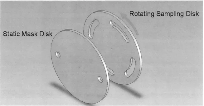
If high frame rate operation using only two horizontally opposed sampling positions is desired, a

rotating disk with several elongated apertures can be used in conjunction with a fixed mask with two aperture holes as shown in Figure 2.4. Increasing the number of elongated apertures on the

rotating disk has the effect of reducing the required motor speed for a desired frame rate, while elongating the aperture arc has the effect of increasing the exposure time for a given frame rate.

Rotating ,afmpfing Disk

Figure 2.4. Schematic of a static two aperture mask in conjunction with a rotating sampling disk. The rotating disk has four elongated apertures which allow for a reduced rotation speed for a given image frame rate. The length of the elongation and the operating frame rate determine the exposure time of each image. The separation between the two disks is exaggerated for clarity.

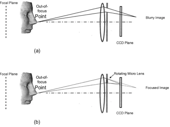
Another approach is to modify the rotating aperture by filling the aperture hole with a small lens (Figure 2.5). The effect of this lens is to converge the sampled rays so that target features very far from the in-focus plane appear in-focus on the imaging plane. In effect, the microlens shifts the in-focus region of Figure 1.6 from a depth band surrounding the in-focus plane to a depth band further away from the in-focus plane, as is shown in Figure 2.6. This new depth band falls on a section of the curve with a higher slope and therefore a higher sensitivity to depth. It is important to note, however, that this same increase in sensitivity to depth can be achieved by simply moving the in-focus plane closer to the lens by focusing it. Though the latter adjustment does in theory reduce the field of view, the reduction is so small as to not have a great effect in practice.

Focal Plane Out-of-focus Point CCD Plane

(a)

Rotting Micro Lens

"11

..-CCD Plane

Focused Image

(b)

Figure 2.5 (a) Standard mechanical AWS implementation. In this case, the target feature is so far in front of the focal plane that the sampled image is blurry, leading to poor processing performance. (b) Rotating micro-lens implementation. Here, the same target feature is perfectly focused onto the CCD plane by the converging lens located inside the rotating aperture. Processing performance is optimized and the system depth sensitivity is increased.

0.4

0

0 0.5 1 1.5 2 2.5 3 3.5 4 4.5

Zt/ZfP

Figure 2.6. Effect of using a microlens in the AWSM. This figure plots the dimensional disparity diameter vs. the non-dimensional target distance from the focal plane. The in-focus range of the original optical system (blue lines) is shifted by the rotating lens further away from the focal plane (red lines), to a region whose greater slope indicates an increased sensitivity to depth.

Focal Plane

d

D

2.4 Electronic Implementation of AWS

The AWS approach can also be implemented electronically. One way to do this is to replace the mechanical aperture with an LCD plane, whose elements can be switched on and off in the shape of an aperture at various locations on the plane. This approach can potentially control both the size and the position of the aperture without any moving parts, and with short response times. One important disadvantage with this approach, however, is that at least 50% of the sampled light is rejected due to the polarization inherent to the LCD technology. Another disadvantage with LCD's is that they have a low fill-factor. This is the percentage of the panel area that actually transmits light, and is typically less than 70% for LCDs. This low fill-factor can have the effect of both reducing the amount of light reaching the sensor plane and of degrading the quality of the image itself.

A second electronic solution to the sampling problem is the use of a Digital Micromirror Device

shown in Figure 2.7 (a). This device, developed and marketed by Texas Instruments, is an array of small mirrors whose tilt can be individually controlled electronically. By placing such a device at an angle to the optical axis, as shown in Figure 2.7 (b), and by turning on specific mirrors so that they reflect light onto the CCD, a wavefront sampling effect can be obtained.

Like the LCD version described earlier, the micromirror approach offers flexible control of both the aperture size and position, but has the added benefit of allowing more light to hit the CCD since the mirror reflectivity is approximately 88% and the chip fill factor is approximately 90%. One disadvantage of the micromirror approach, however, is that the necessity of placing the sampling plane at an angle may introduce some vignetting. This is due to the fact that the wavefront sampling is occurring at different axial positions depending on where the aperture is moved, and as we saw in Figure 2.2 this can lead to some parts of the target disappearing from view depending on the position of the aperture.

(a)

CCD Plane

Point 1

Point 2 Activated Area of Micromirror Array

(b)

Figure 2.7. (a) The Digital Micromirror Device (DMD) is a chip that can hold more than 1 million tiny mirrors on it. The whole chip appears to be a normal mirror to the naked eye. Each 14- Lm2 binary mirror can tilt +12 or -12 degrees when a voltage is applied to its base, resulting in different reflecting directions of the same incident light. Based on whether these mirrors are switched on or off, the

CCD sees dark or bright areas reflected off the DMD (http://www.dlp.com ). (b) Schematic of a micromirror based AWS system.

The computer-controlled micromirror array selectively reflects the incident light onto the CCD camera.

2.5 Illumination of Target

The illumination of the target to be modeled can be critical to the output of high quality 3D results. Structured or random patterns can be projected onto the surface of the target so as to increase its signal to noise ratio, and a variety of different kinds of projectors can be used for this purpose (from simple slide projectors to computer projectors). One key design feature is to align

-- ui. - . =-.--- - - ---

-the illumination source with -the imaging optical train as much as possible. This step insures that shadows on the target are minimized and that the entire target is illuminated as uniformly as possible. Indeed, the best possible solution is to have coaxial illumination, as shown in Figure

2.8. In this conceptual design, the light from the illumination source travels down the same path

as the light from the target. Besides minimizing shadows, this approach also reduces the overall bulk of the system and eliminates the need to separately aim the imaging system and the pattern projector at the target.

In terms of the best design for the projected pattern, its spatial frequency and contrast should be adjusted in order to maximize overall system performance. This will be discussed in detail in Chapter 3.

Figure 2.8. Exploded view of the conceptual design of the 3D monocular system. A readily changeable commercial lens views the object space. The computer-controlled micromirror array selectively reflects the incident light onto the CCD camera. A set of relay

lenses determines the position of the micromirror array along the optical path to ensure optimum imaging quality. Coaxial illumination unit consisting of a 50% beam-splitter, a pattem generator that adds texture onto the object surface and a white light illuminator projects light onto the object being imaged. Courtesy of Dr. Sheng Tan, MIT Hatsopoulos Microfluidics Laboratory.

2.6 Implementation Using 50mm Nikorr Lens

In order to explore the 3D surface imaging capabilities of Active Wavefront Sampling, a system was implemented using a f/1.2 50mm Nikorr lens, a mechanical rotating aperture module, and a Dalsa 1024A CCD camera. The Dalsa camera has a 1024x1024 pixel sensor, with 12 micron pixels, and has an 8 bit grayscale dynamic range. The CCD can be binned down to a 512x512 pixel resolution, and random noise is listed to be approximately 1 Digital Number (DN) by Dalsa

(where the full range is given by 256 DN). The camera is connected to a Coreco Imaging Viper Digital capture card, allowing a 30 Hz frame rate.

Several rotating aperture AWS modules were designed and built over the course of this project, (see Figure 2.9) but all work presented in this thesis using the 50mm Nikorr lens was accomplished using a simple belt driven design built by the Industrial Technical Research Institute (ITRI), in Taiwan ROC. This module, shown in Figure 2.10, mounts the aperture sampling disk on a ball-bearing supported and belt driven gear. The axial position of the rotating aperture sampling disk can be adjusted, and a second fixed sampling mask can be mounted in front of the rotating sampling disk if needed. As was mentioned before, this optional fixed mask serves the purpose of accurately positioning the sampling locations, as well as of removing any smearing caused by the rotating aperture disk moving during the exposure time of the image being acquired. This latter role becomes more important as the speed of rotation increases in an effort to increase the system frame rate. The rotating aperture disk has a single aperture hole with a diameter of approximately 1.5 mm, located at a radial position of 4 mm from the axis of rotation. It was found that increasing the radial position of the aperture any more than this would introduce large amounts of vignetting in the images.

(a) (b)

Figure 2.9. (a) Prototype mechanical AWS module designed for use with an optical train specially designed for monochromatic laser illumination. The aperture disk is driven by a small stepper motor connected via a plastic belt. (b) Compact mechanical AWS module using a ring type DC motor and optical encoder for position feedback (designed by J. Rohaly, Hatsopoulos Microfluidics Laboratory)

Figure 2.10. (a) Exterior view of ITRI designed AWS module, mounted between the Dalsa CA-D4 camera and the Nikkor 50 mm lens. Wires from the stepper motor can be seen protruding from the back of the main casing. (b) Internal view of the same AWS module, achieved by removing the lens and front housing. This view shows the pinion gear, drive belt, and spur gear to which is attached the aperture disk (seen here having a single offset aperture hole). Also visible here is the Hall sensor located between the pinion and spur gears, as well as the metal lip on the spur gear which triggers the zero angular position signal.

The aperture assembly is driven by a Haydon Switch and Instrument, Inc. 36540-12 stepper motor, which is controlled by an Advanced Micro Systems, Inc. MAX-410 controller. The stepper motor is rated at 24 steps per revolution, and the gearing of the motor pinion gear to the aperture spur gear is 10:75. This yields a final aperture angular resolution of 1 degree per motor step when in half-stepping mode. The maximum sustained speed of the stepper motor is

module, and its role is to provide a zero position for the rotating aperture. Before images are acquired, the rotating aperture is moved until a signal from the Hall sensor is received. This angular position is defined as the zero position and the angular position of the aperture is determined by the number of steps taken by the motor relative to this zero position. Though, the overall motor control of the system is clearly open loop, a large number of system tests have shown that the positioning of the aperture to be both accurate and robust.

One end of the AWS module has a standard Nikon F-mount to secure the lens, while the other end is threaded so as to screw into the M42x1 thread on the Dalsa camera. The module thickness is such that the distance between the rear of the Nikkor lens and the CCD plane on the camera is approximately 46.5 mm, the standard F-mount distance. This distance insures that the Nikkor lens is operating under the same conditions it was designed for.

Illumination of the target was performed by using a standard computer projector. One projector that has been used is a 3 LCD type manufactured by Toshiba. A second projector that has also been used is a Digital Light Projection type manufactured by InFocus. This projector uses a single Texas Instruments micromirror array with a spinning color wheel to project an image. It has higher brightness and contrast ratio than the LCD model, and it is also smaller and less bulky. However, it was found that for short camera exposure times (less than 20-30 msec), the brightness variation from one captured image to the other became very large. This suggests that the response time of the single micromirror array combined with the spinning color wheel becomes too long for operating conditions below 20-30 msec. For longer exposure times, however, the captured images showed very uniform brightness using this projector.

A photo showing a typical complete hardware setup for the acquisition of images with the AWS

module is shown in Figure 2.11 below.

Figure 2.11. Photo of complete system setup, with the ITRI AWSM mounted between the Dalsa camera and the Nikkor 50 mm lens, the stepper motor driver, and the 3 LCD projector. The inset image in the top right corner shows a dot pattern being projected onto the target, in this case a human size mannequin head.

Chapter 3: Image Processing

3.1

Introduction

As was discussed in the previous chapters, the Active Wavefront Sampling (AWS) technique encodes depth by shifting the position of a given target's image as a function of the aperture's position on the aperture plane. For the simplest case of a rotating off axis aperture as used in this work, a target point's image will appear to rotate on the image plane as the aperture moves from one angular position to another. Under ideal non-aberrated conditions, the diameter of this circular rotation directly determines the depth of the target point as was shown in Equation 1.6. In order to quantify a target point's depth, therefore, the diameter of this rotation needs to be estimated very accurately by tracking the image motion from one aperture position to the next. In this chapter, background information on some of the various types of tracking algorithms described in the literature will be given, and the algorithms developed specifically for AWS image processing will be described. In describing the algorithms developed for an AWS application, it will be assumed in this chapter that the system's optical train is aberration free. This assumption will be removed in Chapter 4, where the effects of optical aberrations will be incorporated.

3.2

Review of Motion Tracking Algorithms

A large body of work concerning algorithms that track feature motion between image frames

exists. An excellent review of the subject was performed by Barron and Fleet [4]. In this section, several of the most important approaches to the problem will be discussed, including block matching algorithms, frequency domain approaches, as well as gradient methods. The

3.2.1 Block Matching Algorithms

Block matching algorithms are perhaps the simplest form of motion tracking that can be performed. In this approach, the image is divided into small regions (interrogation areas) which are then individually tracked from one image to the next. Matching of the interrogation areas between images is performed by minimizing an error function such as:

Error = j (C[ I+,y,to ),I+ d,,y+ d,,tj)]

(x,y)eR

(3.1) In this expression, R is the region defined by the interrogation area, (d ,, d,) is the displacement

vector, I(x,y, t) is the intensity of the image at given spatial and temporal coordinates, and C[] is a function that indicates the amount of dissimilarity between the two arguments (Lim [5], Little and Verri [6]). Two commonly used choices for video processing applications are the squared difference or the absolute value of the difference between the two arguments

Error= j j[I,y,to--I +d,,y+d,,ti 2

(x,y)eR

(3.2)

Error = (I(xIyIto) _{- I+ + dX ,y + d,,9t)}

(x,y)ER

(3.3)

For each interrogation area in the first image, the error is calculated for a range of displacements in both the x and y directions in the second image. The displacement whose error value is the

smallest is chosen as the true displacement of that particular interrogation area. Block matching in this way can only calculate integer displacement values; in order to calculate subpixel displacements, the original images need to be interpolated so as to provide a finer mesh to the block matching algorithm. Block matching approaches in general can be extremely computationally intensive, especially for long search lengths and for finely interpolated intensity images.

Another evaluation function used to match interrogation areas from one image to another is the discrete cross-correlation function

#(d,,

Xh = YhI(x,y, to) -I(x + dx,,y + d,,5ti )

p(d,d, ) =

Xh ZYh I(xy, t )I Xh _{Y I(x}

_{+ d,y + dt)}

(3.4)

The cross-correlation function approaches 1 when the match between the interrogation area in the first and second images is perfect, and goes to zero where there is no match. Again, the cross-correlation function is calculated for a range of displacements in the x and y directions, so that a cross-correlation table is produced (see Figure 3.1). The displacement vector corresponding to the highest peak in the correlation table is taken to be the actual displacement of the interrogation area. This algorithm is very popular in the experimental fluid mechanics community, where it is used to process images obtained from Digital Particle Image Velocimetry (DPIV) experiments (Willert and Gharib [7]). Just as with the previous metrics, subpixel displacements can be evaluated by first interpolating the original intensity images to a finer grid. Another subpixel approach that avoids interpolation is to fit a Gaussian curve on the correlation plane peak and use the real-valued center of the Gaussian curve as the interrogation area displacement. In order to