• Aucun résultat trouvé

Active vibration cancellation of tonal disturbance using orthogonal eigenstructure control

N/A
N/A
Protected

Academic year: 2021

Partager "Active vibration cancellation of tonal disturbance using orthogonal eigenstructure control"

Copied!
10
0
0

Texte intégral

(1)

Active vibration cancellation of tonal disturbance

using orthogonal eigenstructure control

The MIT Faculty has made this article openly available.

Please share

how this access benefits you. Your story matters.

Citation

Rastgaar, M., M. Ahmadian, and S. C. Southward. “Active vibration

cancellation of tonal disturbance using orthogonal eigenstructure

control.” Active and Passive Smart Structures and Integrated

Systems 2009. Ed. Mehdi Ahmadian & Mehrdad N. Ghasemi-Nejhad.

San Diego, CA, USA: SPIE, 2009. 728823-9. © 2009 SPIE

As Published

http://dx.doi.org/10.1117/12.815639

Publisher

Society of Photo-Optical Instrumentation Engineers

Version

Final published version

Citable link

http://hdl.handle.net/1721.1/52629

Terms of Use

Article is made available in accordance with the publisher's

policy and may be subject to US copyright law. Please refer to the

publisher's site for terms of use.

(2)

Active vibration cancellation of tonal disturbance using

orthogonal eigenstructure control

M. Rastgaar

a

, M. Ahmadian

*b

, S. C. Southward

b

a

Department of Mechanical Engineering, Massachusetts Institute of Technology,

Cambridge, MA, 02139;

b

Center for Vehicle Systems & Safety, Virginia Polytechnic Institute and State

University, Blacksburg, VA, 24060

ABSTRACT

Orthogonal Eigenstructure Control (OEC) is a novel control method that can be used for active vibration cancellation. OEC is an output feedback control method applicable to multiple-input, multiple-output linear systems. In this paper, application of OEC for active vibration cancellation in a plate is presented. A steel plate clamped at four edges is used as a test plate and piezoelectric actuators are used as control actuators. Accelerometers are used for measuring the acceleration and displacement at ten locations on the plate. A tonal disturbance with a frequency of 150 Hz is applied to the plate by an electromagnetic actuator. After identification of the state-space model of the plate, orthogonal eigenstructure control is used to find the control gains that decouple the modes of vibrations and reduce transferring of vibrational energy between them. The results show significant vibration suppression throughout the plate.

Keywords: orthogonal eigenstructure control, active vibration cancellation, structural vibration, plate

1. INTRODUCTION

Eigenstructure assignment methods are effective tools for active vibration cancellation; however, their applications depend on the experience of the control designer based on the geometry and dynamics of the system. For example, they need a definition of the loop eigenvectors and locations for the closed-loop eigenvalues of the closed-closed-loop system, where predicting those values are difficult or will not necessarily lead to a desirable outcome. The main reason is that the closed-loop eigenvectors must lie within the achievable eigenvector set, while a desirable closed-loop eigenvector, suggested by the control designer, may not lie in this set when the dimension of the system is large.

The idea of eigenstructure assignment was initiated by Moore [1, 2]. He showed that there is a class of eigenvectors associated with a distinct set of closed-loop eigenvalues; thus, there are infinite number of control gains or eigenvector matrices for some given closed-loop eigenvalues. A numerical method developed by Cunningham [3] utilized singular value decomposition to find the vectors that span the null space of the eigenvectors of the closed-loop systems. Shelly et al. showed analytically that the absolute displacements in isolated areas in structures can be reduced by eigenvector shaping, regardless of the type of the disturbance [2, 4, 5] and proposed SVD-eigenvector shaping. This method uses a Moore-Penrose generalized left inverse to produce the closest eigenvector in a least square sense to the desired ones [6]. Slater et al. [7] showed that changing the eigenvectors while there is a constraint to keep the closed-loop eigenvalues close to the open-loop ones may lead to excessive control efforts. They showed that a large change in eigenvectors may need a large movement of the eigenvalues to minimize the feedback gains. They also showed that closed-loop eigenvalues have to be consistent with the eigenvectors to avoid large control efforts. Furthermore they suggest that the minimum number of constraints should be imposed to the eigenvectors’ elements to limit the control effort to a reasonable amount.

(3)

Orthogonal eigenstructure control is a novel approach proposed by the authors [8-12], as an active vibration cancellation method that is relatively easy to design and implement. OEC is an output feedback control applicable for structural vibration cancellation. This control method defines a set of desirable closed-loop eigenvectors that decouple the modes of the structure, reject the disturbances, and minimize the spillover of energy from one mode to another. In this method the closed-loop eigenvectors are orthogonal to the open-loop eigenvectors to the feasible extents while they belong to achievable eigenvector set. Therefore, a pre-determination of the closed-loop eigenstructure is not required and no unnecessary constraints are applied to the eigenvectors. Also, eigenstructure assignment methods offer a large and complex design space of options that may overwhelm a designer. To overcome this issue, OEC significantly simplifies the design task and at the same time allows utilizing some experience-based design freedom.

The paper is organized as follow. In section 2, the mathematical basis of the orthogonal eigenstructure control is explained briefly. Section 3, describes the test setup and the components that are used for the experiment. In section 4, the results of the active vibration cancellation in a steel plate due to a tonal disturbance at 150 Hz are explained. Finally, the results of orthogonal eigenstructure control for vibration cancellation are summarized in the conclusion section.

2. MATHEMATICAL EXPLANATION OF OEC

Let’s consider the equation of motion of a first order linear system:

x Ax Bu Ef

&

=

+

+

(1)

y Cx

=

(2)

u Ky

=

(3)

A

is the

N N

×

state matrix and for simplicity,

m

collocated actuators and sensors are considered.

B

is the input matrix,

E

is the disturbance input matrix,

f

is the disturbance vector,

u

is the input vector,

y

is the output vector, and

C

is the output matrix with proper dimensions. Finally,

K

is the

m m

×

feedback gain matrix. The eigenvalue problem for the closed-loop system is defined in matrix notation as

[

| ]

i

0

1, 2,...,

i i

A

I

B

i

N

KC

φ

λ

φ

=

=

(4) i

φ

is the closed-loop eigenvector of the system,

λ

i is the operating eigenvalue, and

I

is the identity matrix. It is seen that the i

i

KC

φ

φ

belongs to the null space of the matrix

S

λi

=

[

A

λ

i

I

| ]

B

N N m×( + ).

Singular value decomposition of

S

λi yields

*

( ) ( ) ( )

[ ]

[ | 0

]

[ ]

i i N N i N m N N m i N m N m

S

λ

=

U

×

Σ

× × +

V

+ × + (5)

The operating eigenvalues are the open-loop eigenvalues. When the open-loop eigenvalues with greatest distance from the origin are chosen as the operating eigenvalues, a more desirable closed-loop system can be achieved [8, 10, 13]. The index

i

is used to specify the equation for the

i

th operating eigenvalue. The number of operating eigenvalues is the same as the number of the required pairs of actuators and sensors

m

.

U

i and

V

i are the left and right orthonormal matrices respectively, and

V

i* is the conjugate transpose of the complex matrix

V

i. If

V

i is partitioned, then the second column block of

V

i spans the null space of the

S

λi [8, 10, 14].

(4)

11 12 ( ) ( ) 21 22

[ ]

[

]

[ ]

[

]

[

]

i i N N N m i N m N m i i m N m m

V

V

V

V

V

× × + × + × ×

= ⎢

(6)

Any linear combination of

m

columns of

V

12i is an eigenvector within the achievable eigenvector set of the closed-loop system.

12

a i i

i

V r

φ

=

(7)

where

φ

ia is an achievable eigenvector of the closed-loop system and

r

iis a coefficient vector that needs to be determined. The corresponding control gain matrix

K

is defined as

22 a i i i

KC

φ

=

V r

(8) * 12 12 i i

V V

and

V V

22i* 22i are Hermitian matrices since

V

12i and

V

22i are complex; therefore, their eigenvalue decompositions yields * * 12 12 i i i i i

V V

=

U

Λ

U

(9) * 22 22 i i i i i w w w

V V

=

U

Λ

U

(10)

where

Λ

i,

U

i and

Λ

iw,

U

wi are the eigenvalue and eigenvector matrices of

V V

12i* 12i and

V V

22i* 22i

respectively. It has been shown by the authors that the eigenvalues of the Hermitian products

V V

12i* 12i and *

22 22

i i

V V

belong to the

[0 1]

interval. It has also been shown that the eigenvectors of

V V

22i* 22i and

V V

12i* 12i are identical and the summation of the eigenvalues of

V V

12i* 12i and

V V

22i* 22i associated with similar eigenvectors are unity [8-12].

i i w

I

Λ + Λ =

(11) i i w

U

=

U

(12)

Using these properties, we can re-arrange equation (9) as

* *

12 12

i i i i i

U V V U

= Λ

(13)

If

U

Ji is the eigenvector corresponding to the unity eigenvalue of

Λ

i, then

U V V U

Ji* 12i* 12i Ji

=

1

(14) * * 22 22

0

i i i i J J

U V V U

=

(15) equation (15) yields 22

0

i i J

V U

=

(16)

(5)

22 22

0

a i i i i

i J

KC

φ

=

V r

=

V U

=

(17)

It implies that the open-loop system is regenerated. This specific

r

ithat is equal to

U

iJ, generates the open-loop eigenvectors from the null space of the closed-loop eigenvectors associated with the operating eigenvalue

λ

i.

V U

12i Ji is identical to the eigenvector corresponding to the open-loop eigenvalue or the operating eigenvalue. The other eigenvectors associated with non-unity eigenvalues of

V V

12i* 12i are orthogonal to

V U

12i Ji. Therefore, a set of closed-loop eigenvectors orthogonal to the open-loop eigenvectors can be found. Further details about the number of possible closed-loop systems as the outcome of orthogonal eigenstructure control can be found in [8, 9, 11, 12].

This process is repeated to the number of pairs of actuators and sensors, and all the calculated closed-loop eigenvectors for entire operating eigenvalues are appended to define

V

and

W

matrices

1 1 12 12 m m

V

= ⎣

V r

L

V r

(18) 1 1 22 22 m m

W

= ⎣

V r

L

V r

(19)

The feedback gain matrix

K

is determined as

1

(

)

K W CV

=

− (20)

Finally, the state matrix of the closed-loop system is

c

A

= +

A BKC

(21)

3. EXPERIMENTAL SETUP

A standard 20-gauge galvanized steel test plate, shown in Figure 1, is clamped to the frame at its four edges. The plate size is 600mm by 500mm. The clamping area is 50 mm at each edge; therefore, the size of plate that it’s dynamic is taken into account for the test is 500mm by 400mm. A bridge is mounted on top of the test stand, to hold the electromagnetic actuator.

The electromagnetic actuator is used for applying the disturbance input to the plate. A stinger made of a threaded rod is used to transfer the force and displacement from the actuator to the plate. At the tip of the stinger a Nylon spacer is placed and glued to the plate to provide a smooth contact area. The stinger is glued 85 mm from the right edge on the axis of symmetry of the short side of the plate. The drive unit amplifier of this actuator can be driven by an external oscillator and may be regarded as an operational amplifier with a voltage gain of unity from DC to 10 kHz.

The control actuators are two high performance piezoelectric actuators T234-A4CL-503X from Piezo Systems, Inc. The piezoceramic elements are composite reinforced bending bimorphs made of PSI-5A4E and have thickness of 0.034 in, an area of 2.5 in by 1.25 in, and weight of 9.7 g. It is X poled for series bending operation. The rated voltages of the piezoceramics are ±250 V. One of the piezoelectric bimorphs is placed at the center of the plate and the second one at a distance of 100 mm away from the first one along the large dimension of the plate. The distance between the second piezoelectric actuator and the electromagnetic actuator is 85 mm. The piezo-driver is a two channel non-inverting high voltage amplifier PZD700 manufactured by Trek. The output voltage of the piezo-driver is within 0 to ±700 V with a current range of 0 to ±100 mA. The amplifier has an adjustable output gain 0 to 300 V/V and has a signal bandwidth of greater than 50 kHz for all voltage ranges.

(6)

0'

Figure 1. Test plate mounted on the frame structure; there are 10 accelerometers and 2 piezoelectric actuators mounted on the plate. Electromagnetic actuator is used as a source of disturbance.

PCB accelerometers with nominal sensitivity of 100 mV/g are used to measure the acceleration at 10 locations on the plate. Seven accelerometers are placed on the top surface of the test plate and three of the accelerometers that are collocated with the actuators are mounted on the lower surface of the test plate. The accelerometers are equally spaced in the transversal direction which is 100 mm. Sensors 1, 2, and 3 are collocated with actuators and are placed at the bottom side of the plate. For signal conditioning, a 20 channel ICP 584 series signal conditioner from PCB Piezotronics, Inc. is used. Finally, for collecting data and output control signals, an AutoBox containing a DS 100e processor, an analog to digital converter DS2201ADC, a digital to analog converter DS2201DAC, and an I/O card with twenty inputs and eight outputs are used.

4. CONTROL OF TONAL DISTURBANCE

To control the induced vibrations to the plate, a model of the system is needed. We intend to apply a tonal disturbance with a frequency of 150 Hz to the plate to validate the OEC effectiveness. A frequency of 150 Hz is chosen because it is one of the natural frequencies of the plate and the coherence of the frequency responses between the disturbance and different accelerometers are high. Figure 2 illustrates the frequency response and its coherence between the acceleration at the electromagnetic actuator location (accelerometer 3) and the accelerometer collocated with the piezoelectric bimorph at the center of the plate (accelerometer 1). For system identification purposes, the piezoelectric actuators are excited by a 150 Hz tonal input signal. The integrated and filtered data from accelerometers 1 and 2 are collected for 6 seconds with 3000 Hz sampling rate. A state space model of the system with a dimension of 10 is estimated. Matlab System Identification Toolbox provides a Prediction-Error Minimization method that is used for system identification [15]. Figure 3 depicts how similar the results of the simulation of the estimated model of the plate are to the collected data with 99% compatibility.

The identified model of the system is used for finding the control gains necessary for the control of vibrations. Orthogonal eigenstructure control is used to find the control gains, and the controller is adjusted by these control gains. Next, the electromagnetic actuator turns on to apply the vibrations with a frequency

accelerometers

piezoelectric

actuators

electromagnetic

shaker

clamped

edges

(7)

50 50 -0 08 06 01 02 50 100 150 200 250 300 350 400 Frequency Response Coherence 50 100 150 200 250 300 350 400 Frequency Hz

of 150 Hz to the plate structure. After 2 seconds, the controller turns on in order to close the feedback control loop and the piezoelectric actuators begin to induce the control force to the system.

Figure 5 shows the signals’ input to the actuators. While the input to the electromagnetic actuator is a steady 150 Hz sinusoidal signal throughout the entire 6 seconds of the experiment, controller signals to the piezoelectric actuators increase from zero to the level that are needed to apply the proper control force. Figure 6 shows the signals from the 10 accelerometers after filtering and converting to displacement. The suppression of vibrations occurs at all the locations. Table 1 shows the maximum amplitude of signals read at accelerometers with and without control. The maximum and minimum amounts of reduction of vibrations are at locations 6 and 9, respectively. The maximum reduction of the amplitude of vibrations is 88.49% and the minimum amount of vibration reduction is 27.80%. The average reduction of amplitude of vibrations throughout the plate is 56.6%.

Figure 2. Frequency response and coherence between the accelerometer collocated with electromagnetic actuator (accelerometer 3) and the accelerometer collocated with piezoelectric actuator at the center of the plate (accelerometer 1)

(8)

04 3.045 3.05 3.055 Time (second) .06 .065 Measured Estimated; fit: 99.88% Measured Estimated; fit: 99.78% 5 5 5 N NO 5 0.05 w 0 0.05 0 2 3 4 5 6 0 2 3 4 5 6 0 2 3 Time (second) 4 5 6

Figure 3. Comparison of results from estimated model and collected data at accelerometer locations for the 150Hz tonal excitations; y1: accelerometer 1; y2: accelerometer 2.

5. CONCLUSIONS

An experiment for validation of applicability of orthogonal eigenstructure control is conducted. The test plate is a steel plate clamped at four edges. A tonal disturbance with a frequency of 150 Hz, generated by an electromagnetic actuator, is applied to the plate. Two piezoelectric bimorphs are used as control actuators and ten accelerometers are mounted on the plate for measuring the vibrations. A state-space model of the plate and the hardware is identified using the measured data. Next, the orthogonal eigenstructure assignment is used to identify the control gains that lead to a closed-loop system with uncoupled modes to the feasible extent. The results show a significant reduction in the maximum amplitude of vibration at all the accelerometers’ locations with an average of 56.6%. This experiment validates the applicability and ease of implementation of the orthogonal eigenstructure control as an active vibration cancellation method.

Figure 4. Signals to the actuators (Volts) for control of 150 Hz disturbance; PZ1: piezoelectric actuator at center of

Controller turned on

Controller turned on

(9)

5 oz -5 5 -5 5 > -5 0

io

-6 x 10 -6 x 10 0) 2 4 6 0 2 4 6 Time (Second) > tu1mp.uum

N-H

2 4 6 0

.

.1

.4

.1

.2.3

Figure 5. Accelerometer Signals (Volts).

Table 1. Comparison of the maximum displacements at accelerometers before and after control (OL: open-loop, CL: Closed-loop)

Accelerometer measurement (V) Maximum OL measurement (V) Maximum CL Percentage reduction

1 2.27e-06 7e-07 -69.10 2 1.01e-06 7.29e-07 -28.20 3 1.56e-06 1.1e-06 -29.75 4 2.33e-06 7.88e-07 -66.23 5 1.19e-06 5.59e-07 -52.85 6 5e-06 5.75e-07 -88.49 7 3.59e-06 7.51e-07 -79.09 8 3.98e-06 1.53e-06 -61.58 9 1.12e-06 8.1e-07 -27.80 10 2.23e-06 8.27e-07 -62.89 REFERENCES

[1] Moore, B., C., "On the Flexibility Offered by State Feedback in Multivariable Systems Beyond Closed Loop Eigenvalue Assignment," IEEE Transactions on Automatic Control, 689-692 (1976).

Accelerometers numbering

(10)

[2] Clark, W., W., Shelley, F., J., "Experiments in Eigenstructure Assignment for Active Mode Localization in a Flexible Beam," Proc. American Control Conference Albuquerque New Mexico, 1859-1863 (1997).

[3] Cunningham, T., B., "Eigenspace Selection Procedures for Closed Loop Response Shaping with Modal Control," Proc. Proc. of the 19th IEEE Conference on Decision and Control Albuquerque New Mexico, (1980).

[4] Corr, L., R., Clark, W., W., "Vibration Confinement Using Piezoelectric Transducers and Eigenstructure Placement," AIAA-99-1552 (1999).

[5] Corr, L., R., Clark, W., W., "Active and Passive Vibration Confinement Using Piezoelectric Transducers and Dynamic Vibration Absorbers," Proc. SPIE Conference on Smart Structures and Integrated Systems Newport Beach California, 3668, 747-758 (1999).

[6] Shelley, F., J., and Clark, W. W., "Active Mode Localization in Distributed Parameter Systems with Consideration of Limited Actuator Placement, Part 2: Simulations and Experiments," Journal of Vibration and Acoustics, 122, 165-168 (2000).

[7] Slater, G., L., and Zhang, Q., "Controller Design by Eigenspace Assignment," AIAA-90-1193-CP, 19-31 (1990).

[8] Rastgaar Aagaah, M., [Vibration Suppression Using Orthogonal Eigenstructure Control], PhD Dissertation Virginia Polytechnic Institute and State University Blacksburg Virginia USA, (2008).

[9] Rastgaar Aagaah, M., Ahmadian, M., Southward, S., C.,"Orthogonal Eigenstructure Control for Vibration Suppression," Journal of Vibration and Acoustics, (2007).

[10] Rastgaar Aagaah, M., Ahmadian, M., Southward, S., C., "Vibration Confinement by Minimum Modal Energy Eigenstructure Assignment," Proc. ASME International Design Engineering Technical Conferences IDETC/CIE 2007 Las Vegas Nevada USA, (2007).

[11] Rastgaar Aagaah, M., Ahmadian, M., Southward, S., C., "Orthogonal Eigenstructure Control with Non-Collocated Actuators and Sensors," Journal of Vibration and Control, (2007).

[12] Rastgaar Aagaah, M., Ahmadian, M., Southward, S., C., "Actuators’ Locations in Vibration Cancellation of a Plate Using Orthogonal Eigenstructure Control," Proc. 18th. International Symposium on Mathematical Theory of Networks and Systems (MTNS08) Blacksburg VA, (2008).

[13] Rastgaar Aagaah, M., Ahmadian, M., Southward, S., C., "Application of Orthogonal Eigenstructure Control to Flight Control Design," Proc. SPIE Smart Structures and Materials & Nondestructive Evaluation and Health Monitoring San Diego CA, (2008).

[14] Shelley, F., J., Clark, W., W., "Experimental Application of Feedback Control to Localize Vibration," Journal of Vibration and Acoustics, 122, 143-150 (2000).

Figure

Figure 1. Test plate mounted on the frame structure; there are 10 accelerometers and 2 piezoelectric actuators  mounted on the plate
Figure 5 shows the signals’ input to the actuators. While the input to the electromagnetic actuator is a  steady 150 Hz sinusoidal signal throughout the entire 6 seconds of the experiment, controller signals to the  piezoelectric actuators increase from ze
Figure 3. Comparison of results from estimated model and collected data at accelerometer locations for the 150Hz  tonal excitations; y1: accelerometer 1; y2: accelerometer 2
Table 1. Comparison of the maximum displacements at accelerometers before and after control (OL: open-loop,  CL: Closed-loop)  Accelerometer  Maximum OL  measurement (V)  Maximum CL  measurement (V)  Percentage reduction  1 2.27e-06 7e-07  -69.10  2 1.01e-

Références

Documents relatifs

In order toimprove, the power factor of the supply network, an advanced control approach based on amultivariable filter is adopted. The novelty of the proposed control

In order to improve, the power factor of the supply network, an advanced control approach based on a multivariable filter is adopted. The novelty of the

Our objective is therefore to determine a feedback controller allowing to significantly reduce the vibration energy in the central zone of the experimental beam when this beam

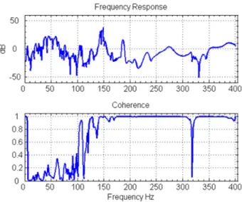
Therefore, a low-order model should refer to a model whose frequency response is close, which means the correspondence around both resonance responses and anti-resonance responses,

Lee, Optimal placement of piezoelectric sensors and actuators for vibration control of a composite plate using genetic algorithms, Smart Materials and Structures 8 (1999) 257–267.

Email address: mohamed.ichchou@ec-lyon.fr (M.N.. phase and gain control policies incorporate necessary weighting functions and determine them in a rational and systematic way; on

Unfortunately, this circumstance may generate a possible increment of the vibration level at other location not managed within the control algorithm; see, in example what has

one max sensor c 2 1i (48) It equals to the output energy measured from the sensors for the ith mode divided by the maximal value of output energy obtained if the ith mode is