Acoustic scattering from sand dollars (Dendraster Excentricus) : modeling as high aspect ratio oblate objects and comparison to experiment

(1)

Author

Joint Program in Oceanography/Applied 0 n ScaenceandEngineerng September 2008

Certified by

Timothy K. Stanton, Senior Scientist Thesis Co-Supervisor A I

" I

Certified by _----

---Andone C. Lavery, Assoc ae Scientist Thesis C&-Supervisor

Accepted by

Alex Techet, Ass'ciae-Piofessor of Mechanical Engineering Chair, Joint Committee for Applig Ocean Science and Engineering

Accepted by

Lallit Anand, Professor of Mechanical Engineering Chairman, Graduate Committee

Acoustic Scattering from Sand Dollars (Dendraster

excentricus): Modeling as High Aspect Ratio Oblate Objects

and Comparison to Experiment

bz

Gregory C. Dietzen

B.S., United States Naval Academy, 2006

Submitted in partial fulfillment of the requirements of the degree of Master of Science

at the MASSACHUSETTS 1I

MASSACHUSETTS INSTITUTE OF TECHNOLOGY OF TECHNOLO

And the

WOODS HOLE OCEANOGRAPHIC INSTITUTION

_{DEC 0}

₇

₂₀₍

September 2008

LIBRARIE

The author hereby grants to MIT and WHOI permission to reproduce and to distribute publicly paper and electronic copies of this thesis document in whole or in part in any medium now

known or hereafter created.

---

,--3Y

8 ST

(2)

(3)

Acoustic Scattering from Sand Dollars (Dendraster excentricus):

Modeling as High Aspect Ratio Oblate Objects and Comparison

to Experiment

Gregory

T.

Dietzen

Submitted in partial fulfillment of the requirements of the degree of Master of Science

at the Massachusetts Institute of Technology and the Woods Hole Oceanographic Institution

Abstract

Benthic shells can contribute greatly to the scattering variability of the ocean bottom, particularly at low grazing angles. Among the effects of shell aggregates are increased scattering strength and potential subcritical angle penetration of the seafloor. Sand dollars (Dendraster excentricus) occur commonly in the ocean and have been shown to be significant scatters of sound. In order to understand more fully the scattering mechanisms of these organisms, the scattering from individual sand dollars was studied using several methods.

Using an approximation to the Helmholtz-Kirchhoff integral, the Kirchhoff method gives an analytic integral expression to the backscattering from an object. This integral was first solved analytically for a disk and a spherical cap, two high aspect ratio oblate shapes which simplify the shape of an individual sand dollar. A method for solving the Kirchhoff integral numerically was then developed. An exact three dimensional model of a sand dollar test was created from computed tomography scans. The Kirchhoff integral was then solved numerically for this model of the sand dollar.

The finite element method, a numerical technique for approximating the solutions to partial differential equations and integral equations, was used to model the scattering from an

individual sand dollar as well. COMSOL Multiphysics was used for the implementation of the finite element method.

Modeling results were compared with published laboratory experimental data from the free field scattering of both an aluminum disk and a sand dollar. Insight on the scattering mechanisms of individual sand dollar, including elastic behavior and diffraction effects, was

gained from these comparisons.

Thesis Co-Supervisor: Tim Stanton Title: Senior Scientist

Thesis Co-Supervisor: Andone Lavery Title: Associate Scientist

(4)

(5)

Acknowledgements

The chance to pursue scientific research at the Massachusetts Institute of Technology and the Woods Hole Oceanographic Institution for the past two years has fulfilled a dream. I will forever be grateful to the Navy for providing me the opportunity and the funding to make this possible. It has been time well spent!

I am extremely appreciative of the support of my two research advisors at the Woods Hole Oceanographic Institution. Dr. Tim Stanton provided the framework for my work at WHOI with his immense experience in the field of acoustic scattering. The enthusiasm and acumen that he offered have been truly valuable gifts. Dr. Andone Lavery has been a constant source of guidance and tutelage, helping me clear many difficult research hurdles. Her insight and tireless assistance were always more than enough to encourage me to continue forward.

This thesis would not have been possible without the help of Dr. Gonzalo Feijoo. His generous donations of time and energy helped introduce me to the powerful and challenging world of modem numerical analysis. Without his insight and contribution of computer resources, the necessary finite element method calculations would have been impossible. I am also grateful to Dr. Dezhang Chu who provided the experimental data that was such a key component of my work.

I would not be where I am today without my parents, who very early taught me the value of filling "the unforgiving minute with sixty seconds worth of distance run." Their unwavering love and support have been a steadfast source of strength. The rest of my family, especially my sister Mary Devon and brother Peter, have continued to help with challenges on the road ahead by reminding me of where I come from.

So many friends, old and new, have been a part of my life over the past two years. I know I will always remember fondly the time that I spent with them in Cambridge and Woods Hole. Finally I would like to thank my amazing girlfriend, Maya, for her encouragement and support in everything that I do. Daisuki desu.

(6)

(7)

List of Figures

Figure 1 - Photograph of sand dollar test, top-view (Stanton and Chu, 2004)...18

Figure 2 - Spherical coordinate system, shown with incoming wave and without scatterer geom etry. ... 27

Figure 3 - Target strength of a rigid/fixed sphere of radius 5 cm, from the Kirchhoff method (starred line) and modal senes solution (smooth line). ... 29

Figure 4 - Cylindrical coordinate system, shown with incoming wave and without scatterer geom etry ... 31

Figure 5 - Broadside target strength of a rigid/fixed finite cylinder of length 10 cm and radius 1 cm using the Kirchhoff method (starred line) and modal series approximation (solid line). Figure 6 - Geometry of the infinitely thin disk ... 36

Figure 7 - Geom etry of the disk. ... ... 38

Figure 8 - Geometry of the spherical cap. ... 40

Figure 9 - Examples of minmax tests in x for Newell's algorithm...44

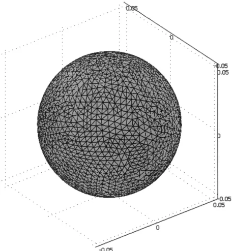
Figure 10 - Surface mesh of a sphere of radius 5 cm in COMSOL...46

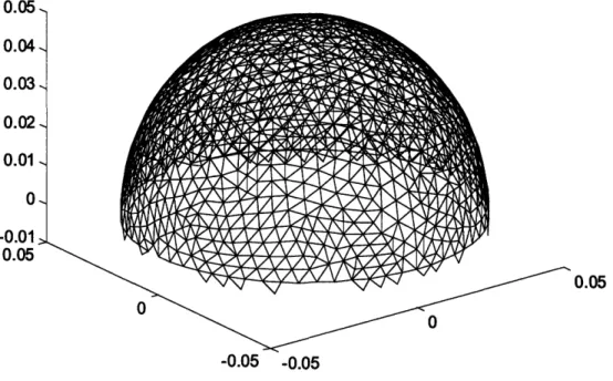
Figure 11 - Surface mesh of a sphere in MATLAB after Newell's algorithm...47

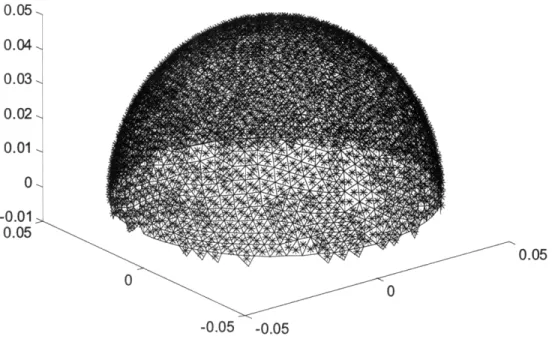
Figure 12 - Surface mesh of a sphere in MATLAB after Newell's algorithm, with triangle m idpoints...48

Figure 13 - Close view of surface mesh of sphere, with midpoints...48

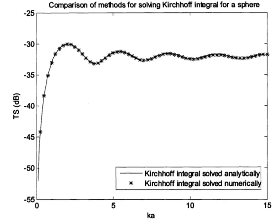
Figure 14 - Target strength of a rigid/fixed sphere with radius 5 cm by solving the Kirchhoff integral analytically (solid line) and numerically (stars) ... .... 49

Figure 15 - Surface mesh of a finite cylinder in COMSOL... ... 50

Figure 16 - Surface mesh of a finite cylinder in MATLAB after Newell's algorithm...50

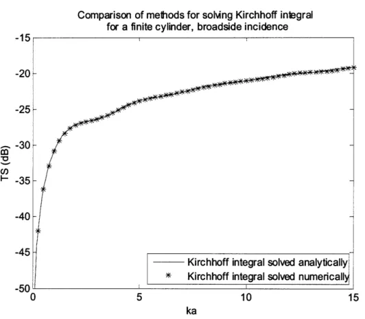
Figure 17 - Target strength of a rigid/fixed finite cylinder with length 10 cm and radius 1 cm by solving the Kirchhoff integal analytically (solid line) and numerically (stars)...51

Figure 18 - Surface mesh of a disk in COMSOL ... 52

Figure 19 - Surface mesh of a disk in MATLAB after Newell's algorithm...53

Figure 20 - Target strength of a rigid/fixed disk with radius 5 cm and thickness 1 cm by solving the Kirchhoff integral analytically (solid line) and numerically (stars) ... 54

Figure 21 - Surface mesh of a spherical cap in COMSOL. ... 55

Figure 22 - Surface mesh of a spherical cap in MATLAB after Newell's algorithm ... 55

Figure 23 - Target strength of a rigid/fixed spherical cap with radius 5 cm and radius 1.34 cm by solving the Kirchhoff integral analytically (solid line) and numerically (stars)...56

Figure 24 - Domain of three dimensional scattering problem, shown with incident wave...59

Figure 25 - Geometry of a bounded three dimensional scattering problem...60

Figure 26 - Examples of two linear (left) and three quadratic (right) triangular finite elements, used to discretize two dimensional problems. The black dots represent the positions of the nodes ... ... . ... 64

Figure 27 - Example of a three dimensional quadrilateral quadratic finite element. The black dots represent the positions of the ten nodes...64

Figure 28 -Sample three dimensional and two dimensional finite element domains in COMSOL ... ... 77

Figure 29 - Total and scattered pressure fields from a rigid/fixed infinite cylinder, ka = 10 in COMSOL. The incident wave arrives from the left side of the domain ... 83

Figure 30 - Max error norm versus EPW for COMSOL approximation of scattering from a rigid/fixed infinite cylinder at ka = 1... 84

Figure 31 - Max error norm versus EPW for COMSOL approximation of scattering from a rigid/fixed infinite cylinder at ka = 5... 84

Figure 32 - Absolute value of infinite form function of a rigid/fixed infinite cylinder, using the modal series solution and COMSOL (point method). EPW = 6 and SMD = 50 ... 86

Figure 33 - Absolute value of infinite form function of a rigid/fixed infinite cylinder, using the modal series solution and COMSOL (circular integral method). EPW = 6 and SMD = 50. ..87

Figure 34 - Error in the infinite form function approximation of a rigid/fixed infinite cylinder at SM D = 50. ... 88

(10)

Figure 35 - Error in the infinite form function approximation of a rigid/fixed infinite cylinder at EPW = 6...89

Figure 36 - Target strength of a rigid/fixed sphere, radius 5 cm, using the modal series solution and COMSOL (spherical integral method). EPW = 6 and SMD = 20 ... 90 Figure 37 - Target strength at broadside incidence of a rigid/fixed disk of radius 3.625 cm and

thickness 5.5 mm, based on (1) the analytic solution of the Kirchhoff integral (dashed line) and (2) the finite element method using COMSOL with axial symmetry (line with x's). EPW = 6 and SM D = 50. ... ... 94 Figure 38 - Target strength at 70 kHz of a rigid/fixed disk of radius 3.625 cm and thickness 5.5

mm based on (1) the analytic solution of the Kirchhoff integral (dashed line) and (2) the finite element method using COMSOL (line with x's). EPW = 6 and SMD = 20. ... 95 Figure 39 - Cross section of a sand dollar (Dendraster excentricus) obtained from CT scans.

Details of the inner structure are revealed in addition to the high-resolution measurements of the outer shape (from Andone Lavery, personal communication). ... 97 Figure 40 - Companson of measured target strength at 70 kHz as a function of angle of

orientation for an aluminum disk (solid starred line), radius 4 cm and thickness 1.9 mm, to predicted target strength of a rigid/fixed disk of similar dimensions found by solving the Kirchhoff integral analytically (dashed line) ... 99 Figure 41 - Comparison of measured target strength at 70 kHz as a function of angle of

orientation for an aluminum disk (solid starred line), radius 4 cm and thickness 1.9 mm, to predicted target strength of a rigid/fixed disk of similar dimensions using the finite

element method in COMSOL (thin solid line with x's). EPW = 6 and SMD = 20 ... 101 Figure 42 - Three dimensional sand dollar model in COMSOL, with the round side visible. ...103 Figure 43 - Sand dollar surface mesh in MATLAB after implementing Newell's algorithm, with

the orientation corresponding to an incident wave normal to the flat side ... 104 Figure 44 - Comparison of predicted target strength at 70 kHz as a function of angle of

orientation for a rigid/fixed disk, radius 3.625 cm and thickness 5.5 mm, based on the analytic solution of the Kirchhoff integral (dashed line) to predicted target strength of the flat side of a rigid/fixed sand dollar of similar dimensionsbased on a numerical solution to the Kirchhoff integral (solid line with circles)...105 Figure 45 - Comparison of measured target strength at 70 kHz as a function of angle of

orientation for the flat side of a sand dollar (solid starred line), to predicted target strength of a rigid/fixed disk, radius 3.625 cm and thickness 5.5 mm, found by solving the Kirchhoff integral analytically (dashed line) ... 106 Figure 46- Comparison of measured target strength at 70 kHz as a function of angle of

orientation for the flat side of a sand dollar (solid starred line), to predicted target strength of the flat side of a rigid/fixed sand dollar found by solving the Kirchhoff integral

numerically (solid line with circles)...107

Figure 47 - Comparison of measured target strength at 70 kHz as a function of angle of

orientation for the flat side of a sand dollar (solid starred line), to predicted target strength of a rigid/fixed disk of radius 3.625 cm and thickness 5.5 mm using the finite element method in COMSOL (thin solid line with x's). EPW = 6 and SMD = 20 ... 108 Figure 48 - Sand dollar surface mesh in MATLAB after implementing Newell's algorithm, with

the orientation corresponding to an incident wave normal to the round side... 109 Figure 49 - Comparison of predicted target strength at 70 kHz as a function of angle of

orientation for an spherical cap, radius 3.625 cm and thickness 1.1 cm, based on the analytic solution of the Kirchhoff integral (dashed line) to predicted target strength of the round side of a rigid/fixed sand dollar of similar dimensions based on a numerical solution to the Kirchhoff integral (solid line with circles). ... 110 Figure 50 - Comparison of measured target strength at 70 kHz as a function of angle of

orientation for the round side of a sand dollar (solid starred line), to predicted target strength of a rigid/fixed spherical cap, radius 3.625 cm and thickness 1.1 cm, found by solving the Kirchhoff integral analytically (dashed line). ... 111 Figure 51 - Comparison of measured target strength at 70 kHz as a function of angle of

orientation for the round side of a sand dollar (solid starred line), to predicted target strength of the round side of a rigid/fixed sand dollar found by solving the Kirchhoff

(11)

Figure 52 - Geometry of a single layer in between two infinite half spaces...114 Figure 53 - Reflection coefficients from three layer model (calcite-water-calcite). Calcite

thickness refers to both top and bottom layer thickness. ... ... 117 Figure 54 - Comparison of measured target strength at 70 kHz as a function of angle of

orientation for an aluminum disk (solid starred line), radius 4 cm and thickness 1.9 mm, to predicted target strength of a penetrable disk (

I

RL = 0.5954) of similar dimensions found by solving the Kirchhoff integral analytically (dashed line) ... 118 Figure 55 - Comparison of measured target strength at 70 kHz as a function of angle of

orientation for an aluminum disk (solid starred line), radius 4 cm and thickness 1.9 mm, to predicted target strength of an penetrable disk ( I RL I = 0.5954) of similar dimensions using the finite element method in COMSOL (thin solid line with x's). EPW = 6 and SMD = 20.119 Figure 56 - Comparison of measured target strength at 70 kHz as a function of angle of

orientation for the flat side of a sand dollar (solid starred line), to predicted target strength of the flat side of penetrable sand dollar ( I RL

I

= 0.4) found by solving the Kirchhoff

integral numerically (solid line with circles). ... 120 Figure 57 - Comparison of measured target strength at 70 kHz as a function of angle of

orientation for the flat side of a sand dollar (solid starred line), to predicted target strength of a penetrable disk (I RL

I

= 0.4) of radius 3.625 cm and thickness 5.5 mm using the finite element method in COMSOL (thin solid line with x's). EPW = 6 and SMD = 20. ... 121 Figure 58 - Comparison of measured target strength at 70 kHz as a function of angle of

orientation for the round side of a sand dollar (solid starred line), to predicted target strength of the round side of a penetrable sand dollar ( I RL I = 0.4) found by solving the Kirchhoff integral numerically (solid line with circles). ... 122

(12)

(13)

List of Tables

Table 1 - Target information for the acoustic scattering experiment performed by Stanton and

C hu (2004)...96

Table 2 - Comparison summary for aluminum disk ... ... 98

Table 3 - Comparison summary for sand dollar, flat side ... 98

Table 4 - Comparison summary for sand dollar, round side ... .... 98

(14)

(15)

Chapter 1 Introduction

1.1 Sound as a Tool in the Ocean

Sound is an important tool for gaining insight into phenomena and processes in underwater environments. In the ocean, the theory of sound is essential in such broad

applications as military operations, geological exploration, and biological surveys. Unlike electromagnetic waves, acoustic pressure waves are able to propagate long distances in water. The typical frequency range used in underwater acoustics is 10 Hz to 1 MHz, with the lower frequencies able to travel many kilometers. An important aspect of the field is acoustic

scattering, that is, understanding how sound reacts to boundaries and obstacles in its path. With SONAR (Sound navigation and ranging)-a method for marine vessels to navigate,

communicate, and detect one another-as its most well-known application, acoustic scattering includes the study of the reflection, diffraction, and transmission of sound incident upon a particular object. This analysis can often convey detailed information about the nature of the object such as its shape, size, or material properties. Knowledge of scattering mechanisms is important in such diverse applications as mine detection and investigating zooplankton populations. There is a vast literature on the subject of underwater acoustic scattering (Urick,

1983; Medwin and Clay, 1998).

1.2 Scattering from Benthic Shells

The seafloor is a significant scatterer of sound. Not only essential to the determination of bathymetry, knowledge of how sound scatterers from the ocean bottom has commercial,

military, and scientific ramifications. Sediment type, bottom roughness, and grazing angle all are important variables in seafloor scattering. Jackson et al. (1986) presented data showing how sediment type alone is not a good predictor of scattering strength, with variations up to 15 dB within a single class of seafloor material. Jackson and colleagues also showed how seafloor

(16)

roughness seemed to account for high variability in the acoustic returns at shallow grazing angles. An important instance of seafloor roughness is the presence of benthic shelled

organisms. Studies have suggested that the presence of benthic shells can contribute greatly to the scattering strength of the ocean bottom at frequencies above 10 kHz (Stanic et al., 1989;

Fenstermacher et al., 2001). Not only can shells greatly increase the scattering strength in the backwards direction, but they also scatter sound into the seafloor itself. This raises the

possibility of detecting buried objects at subcritical angles (Stanton and Chu, 2004). However, the understanding of benthic shell aggregate scattering remains limited due to an incomplete knowledge of the scattering from individual benthic shells.

Accurately describing the scattering from most marine organisms is a significant

challenge, in part due to their geometric complexities. In particular, there are no exact analytic expressions for the scattering from irregular benthic shells. There are only eleven relatively simple geometric shapes with separable coordinate systems, including spheres and infinite cylinders, and thus with exact analytic solutions to their scattering (Bowman et al., 1969; Anderson, 1950; Faran, 1951). In addition to geometry, material properties are also an

important factor in the scattering physics of an object. These material properties are important in determining proper boundary conditions on the surface of the object. Fluid objects simply require continuity of pressure and velocity on their boundary. Solid objects, referred to as elastic, involve more complicated boundary conditions due to the presence of shear waves. Accurately representing the boundary conditions of an object can be just as important as its geometry in the modeling of its scattering.

There has been much work done regarding the scattering of individual zooplankton, including shelled organisms, in the water column (Simmonds and MacLennan, 2005). Certain animal classes have been approximated as simple geometrical shapes, such as spheres

(Greenlaw, 1977; Johnson, 1977; Stanton et al., 1987; 2000) and finite cylinders (Stanton, 1989; Stanton et al., 1993). More complex representations of certain water-column scatterers have also been used. In particular, scattering models based on the distorted wave Born approximation (DWBA) have proved useful in modeling fluid-like zooplankton (Chu et al., 1993; Stanton et al., 1993, 1998; Stanton and Chu, 2000; Lavery et al., 2002; Lawson et al., 2006, Lavery et al., 2007).

(17)

Compared to the understanding developed for scattering from water-column organisms, relatively little work has been done regarding the scattering from individual benthic shelled organisms. Stanton et al. (2000) used a deformed sphere in both ray-based and modal-series-based approaches to model scattering from periwinkles (Littorina littorea), a type of benthic shelled animal. Stanton and Chu (2004) compared laboratory measurements of scattering from a machined round, elastic disk to that of a sand dollar (Dendraster excentricus) and bivalve

(Dinocardium robustum vanhyningi). Specifically, they observed diffraction effects from the edges of the sand dollar through pulse-compression analysis. Though much progress was made in these studies, understanding the importance of the geometrical complexities of these benthic shelled organisms on the scattering was incomplete, which is the motivation for this study. In particular, the focus of this work is to understand acoustic scattering from sand dollars, for which there are controlled laboratory scattering data available (Stanton and Chu, 2004) that can give insight and inspire model development.

1.3 Scattering from Sand Dollars

Sand dollars (Dendraster excentricus) were shown by Fenstermacher et al. (2001) to contribute significantly to seafloor scattering levels when in naturally occurring dense

collections. These benthic echinoderms can form concentrations of up to several hundred per square meter in the sandy, shallow water of the west coast of North America (Chia, 1969; Highsmith, 1982). Sand dollars have skeletons composed of strong calcite, correctly referred to as tests and not shells because of a small amount of external living tissue (Nichols, 1969). These tests, clearly visible after the animal has died, resemble thin round disks, as seen in figure 1.

(18)

Figure 1 - Photograph of sand dollar test, top-view (Stanton and Chu, 2004).

Sand dollars grow to several centimeters in diameter; Chia's (1969) population records show an average adult diameter of 7 cm. Understanding the scattering from individual sand dollars is important for predicting the scattering from aggregations of live organisms found in situ on the ocean bottom.

This work attempts to further understand the scattering from individual sand dollars by first modeling them as high aspect ratio oblate objects, namely disks and spherical caps. Along with the geometrical complexities, the material properties of sand dollars are important to an accurate description of their scattering. One key simplification to the models developed here is that a rigid/fixed, rather than elastic, boundary condition is used. This removes the

complexities of shear waves and internal structure from the analysis and proves to be a good approximation at certain angles of orientation with an added heuristic reflection coefficient. Though the complex scattering mechanisms of elastic disks have been illustrated by Hefner and Marston (2001), they are beyond the scope of this work. Also, the models' focus is solely on the backscattering of incident harmonic plane waves. Both an approximate analytical technique,

namely the Kirchhoff method, and a fully numerical technique, namely the finite element method, are used to model the scattering from sand dollars. Both techniques model them as simple high aspect ratio oblate objects (disks and spherical caps). The Kirchhoff method is then taken further to model the scattering from the sand dollar's exact geometry, obtained from high

(19)

computed tomography (CT) scans. All work involves free field scattering, that is, the scatterer is away from all boundaries.

1.4 The Kirchhoff Method

The Kirchhoff method is an approximation of the Helmholtz-Kirchhoff integral, derived from the theorems of Gauss and Green. The result of the method is an analytic integral that is evaluated over the insonified surface of the scatterer to determine its reflection. There is a vast literature on the subject in both optics and acoustics (Born and Wolf, 1970; Medwin and Clay, 1998). Because any scattering process often also involves strong diffraction effects, there are limitations to the accuracy of the method. In particular, it loses accuracy as wavelength increases beyond the characteristic dimensions of the object. Norton et al. (1993) studied the diffraction-induced errors of this method in the scattering from circular disks.

In Chapter 2, a brief derivation of the Kirchhoff method is discussed. The resulting integral expression is then solved for two objects: a sphere and a finite cylinder. The results are compared to the sphere's exact modal series solution and the finite cylinder's modal-series-based approximation. Next, the Kirchhoff integral expression is solved for a disk and spherical cap, the two objects that approximate the shape of each side of the sand dollar. Finally, a method for solving the Kirchhoff method's integral numerically is presented. It is based on creating a mesh conforming to the surface of the scatterer and summing the integral over the resulting elements. This approach is valuable because it does not require the object's surface to be separable and thus can be used on arbitrarily complex scatterers. Finally, the numerical

approach is tested against the previous analytic solutions of the Kirchhoff integral for the sphere, finite cylinder, disk, and spherical cap.

(20)

1.5 The Finite Element Method

Broadly defined, a numerical technique is a way of approximating continuous problems with discrete solutions. The idea of numerical analysis arose long before computers, evidenced by very old techniques such as Newton's and Euler's methods. However, the surge in

computing power over the past several decades has greatly expanded the scope and power of using numerical techniques for solving problems. In the context of acoustic scattering, a few distinct numerical techniques have risen in popularity, such as the T-matrix and finite element methods. The T-matrix method is a formally exact numerical solution to the wave equation. Introduced by Waterman (1969), this approach has been used to study the scattering and

diffraction of thin circular disks (Kristensson and Waterman, 1982; Norton et al., 1993; Stanton et al., 2007).

An approach to approximating solutions to partial differential equations and integral equations, the finite element method is a general numerical technique with a broad scope of applications. It stemmed from the work of applied mathematicians, physicians, and engineers in the mid twentieth century; each community was interested in approximating solutions to increasingly complex continuous problems (Huebner, 1975). The first mention of the term "finite element method" was by Clough (1960) to describe plane elasticity. Earlier, Courant (1943) used piecewise continuous functions over triangular elements to study the St. Venant torsion problem. The mathematical foundations of the finite element method were solidified in the early 1970s (Strang and Fix, 1973; Babuska and Aziz, 1973), and it has become a popular numerical technique in a wide variety of fields. Early use of the finite element method in the study of acoustics focused on internal problems such as acoustics of an enclosure, structural vibration, and waveguides (Gladwell, 1966; Craggs, 1972; Nefske et al., 1982; Petyt, et al., 1976). As techniques have been developed to deal with the infinite domain of scattering problems, the finite element method has been adapted for them as well (Hunt et al., 1975; Bettess, 1977; Gan et al., 1993; Berenger, 1994; Thompson, 2006).

In Chapter 3, the theory behind the finite element method and its application to acoustic scattering problems are discussed. Techniques for reducing numerical error in two and three

(21)

dimensions are presented. The program COMSOL Multiphysics@ is then explored for its use in predicting the scattering from sand dollars. The accuracy and limitations of this method are explored by again solving problems with known solutions, scattering from a rigid/fixed infinite cylinder and a rigid/fixed sphere.

1.6 Comparison to Experiment

In Chapter 4, the results from both the Kirchhoff method and finite element method models are compared with published (Stanton and Chu, 2004) experimental results. In Stanton and Chu (2004), forward scattering and backscattering from a sand dollar test, a bivalve shell, and a machined aluminum disk of similar size were measured over a range of angles of orientation. Model results based on the finite element method and analytic and numerical solutions to the Kirchhoff method are compared to the experimental results from the aluminum disk and the two faces of the sand dollar. These comparisons are conducted at a single

frequency, 70 kHz, over a range of angles of incidence.

As the wavelength used is similar in size to the dimensions of the sand dollar and

aluminum disk, certain inaccuracies show up in the use of the Kirchhoff method, as mentioned before. However, near normal incidence to the main faces of the sand dollar and aluminum disk (referred to as broadside), this approach results in good agreement between the predicted and measured scattering. The finite element method is able to model some of the experimental data at higher angles of orientation in addition to working well near broadside. Errors due to the use of a rigid/fixed boundary condition are discussed and a heuristic approach to representing the true penetrable condition of the scatterers by means of an added reflection coefficient is

(22)

1.7 Overview of Study

To summarize, Chapter 2 discusses the Kirchhoff method and the resulting solutions for two shapes similar to a sand dollar. Chapter 3 discusses the finite element method and its application in modeling the scattering by a sand dollar. Chapter 4 compares the results of the models with experimental scattering data for an aluminum disk and sand dollar. A heuristic correction to the models is discussed as well to account for the use of the rigid/fixed rather than elastic boundary conditions. Chapter 5 summarizes the thesis and offers recommendations for future work.

(23)

Chapter 2 The Kirchhoff Method

2.1 Introduction

In this chapter, models for understanding the backscattering from individual sand dollars are created through use of the Kirchhoff method. A brief overview of the Kirchhoff method is presented, which results in an analytic integral, referred to as the Kirchhoff integral, which approximates the backscattering amplitude of an object when exposed to an incident harmonic plane wave. The Kirchhoff integral is tested for two shapes with known solutions, namely spheres and finite cylinders. However, because sand dollars have complicated shapes, for which there are no analytic solutions to the Kirchhoff integral, they are represented in this chapter by objects with simpler geometries that incorporate the sand dollar's high aspect ratio oblate shape, namely round disks and spherical caps. These objects are all rigid/fixed, based on the assumption that this is a good approximation of the sand dollar's boundary condition. Finally, a technique for solving the integral numerically for any shape, regardless of geometric complexities, is presented. Numerical solutions to the Kirchhoff integral are then compared to the analytic solutions for a sphere, finite cylinder, disk, and spherical cap.

2.2 Theoretical Background

The Kirchhoff method's derivation begins with the theory of wave propagation proposed by Christian Huygens. Described in detail by Born and Wolf (1970), Huygens'

principle is that each point on an advancing wave front can be considered a source of secondary spherical wavelets. Together, these wavelets form the new wave front as it propagates. Using the theorems of Gauss and Green, analytic expressions for these wavelets can be written. In scattering problems, these wavelets are analyzed on the surface of the scatterer, resulting in the scattered pressure field. Medwin and Clay (1998) summarize the derivation, giving the

(24)

1. 8 e' ei' 8Pcat (?)l (2.1)

psa:4(1) = Ja IPsa t(') r d, .ah

This is an expression for the scattered pressure at position Fi in terms of its value along the surface of the scatterer, oa. Each differential element do on the object's surface has position F' and outward unit normal . The term r, is the distance from the surface element to position i,

r, =1 - ' and k (= 2;r / A, where A is the wavelength) is the acoustic wavenumber. The Kirchhoff approximation simplifies the integral by assuming that each differential element reflects sound in a ray-like manner; each element behaves just as a part of a tangent infinite planar interface would (Medwin and Clay, 1998). This means that the scattered pressure can be written in terms of the incident pressure and the reflection coefficient R, that would result from such an interface. Implicit in this approximation is that only the insonified or "front" of the object contributes to scattering. The field in the shadow or "back" of the object is zero. Therefore, the integral for the scattered pressure is only evaluated on the scatter's insonified surface, 1 8 eik' (2.2) p sca, ,(X) = R , ( e ( ') L ) 2 d .. 2) 41 a n (r.

To simplify further, the incident field is considered to be a harmonic plane wave, written in its time independent form as Pic (P') = Poeik-r', with amplitude po and wave vector k, where

k = kk and I is a unit vector in the direction of the wave's propagation. (Throughout this work, only harmonic waves are considered, so the time dependence is omitted). Inserting the expression for the incident field into the integral gives

Pscat(i) = Rl . e ikr,) d (2.3)

Two further simplifications are made. First, the scatterer is considered to have a rigid/fixed boundary condition; this is defined as one where both the gradient of pressure and the fluid velocity are zero on the boundary. The reflection coefficient for a rigid/fixed interface is always

(25)

equal to one, regardless of angle of orientation. Second, the scattered pressure is only calculated at a distance from the object much larger than the object's dimensions. To do this, the

coordinate system must be oriented so that the scatterer is located at the origin. Then the distance from the origin to the point i, defined as r = xi , must satisfy r >> d, where d is a

typical object dimension. When this is the case, r is a good approximation of the r, term in the

denominator. The r, in the exponent must be approximated more carefully due to the importance of the phase,

(2.4)

r

When the scattered pressure is calculated in the backwards direction, opposite to the direction of the incident wave, this can be rewritten as,

r r + '.. (2.5)

With these approximations, the backscattered pressure (from equation (2.3)) can be expressed as

a

e i ekr (2.6)

4 r

an

r

The normal derivative of - is assumed to be zero because r is large, giving

r

Skr

ikr )i 2 . (2.7)

an r r

The integral thus reduces to

ik (2.8)

Pbs P0 e n )e i2"'do.

This is the final Kirchhoff method expression for the backscattered pressure. In the far-field kr >> 1, the scattered pressure is defined as

Peikr (2.9)

(26)

where f(Q) is known as the scattering amplitude. It is a function of the spherical angles

represented by 2 . Thus from equation (2.8), the backscattering amplitude, fb,, can be written,

i )e (2.10)

Backscattering amplitude can be used to find target strength (Urick, 1983),

TS = log fbs2. (2.11)

The units of target strength are decibels (dB) relative to 1 m2_{. Target strength is a heavily used} indicator of scattering strength and is based solely on the properties of the scatterer itself. Only backscattering is considered throughout this work, so the subscript bs can be dropped. This expression in equation (2.10) is referred to here as the Kirchhoff integral and can be used to calculate the scattering of an object by performing the integral over its insonified surface.

The Kirchhoff method is also referred to as the physical optics method. By only accounting for reflection from the object's front insonified surface, this method neglects the effects of diffraction. Diffraction effects vary greatly with frequency and object shape, making the Kirchhoff method a poor approximation at times. These effects can be explored by

comparisons with shapes that have known exact solutions or approximations to their scattering, such as spheres and finite cylinders.

2.3 Scattering from a Sphere

In this section, the Kirchhoff integral is solved for a rigid/fixed sphere. The results are compared to the exact modal series solution for scattering from a rigid/fixed sphere.

2.3.1 Kirchhoff Integral Solution for a Sphere

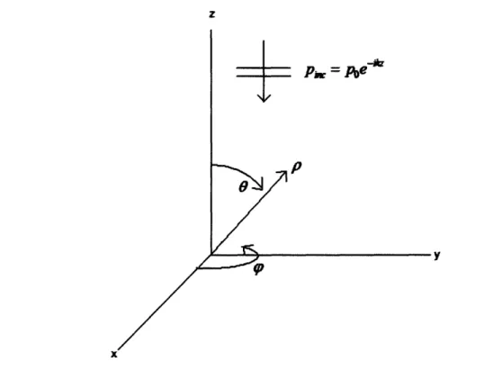
The first step involves setting up a spherical coordinate system with radial variable p, polar variable 0, and azimuth variable p. The Cartesian coordinate system is described with

(27)

unit vectors x, y, and 2. Assume a rigid/fixed sphere with radius a is centered at the origin

and consider an incident plane wave pine = Poe- ik _{proceeding in the negative z direction, as}

seen in figure 2. This orientation is chosen to simplify the limits of integration in the integral. z

y

Figure 2 - Spherical coordinate system, shown with incoming wave and without scatterer geometry.

It is seen that

(2.12)

k = -kd

A = cos p sin 89 + sin (Psin 899 + cos 82 = a cos p sin 89 + a sin r sin 8O+ a cos 89

dor = a2 _{sin OdOdo .}

In this case, the Kirchhoff integral becomes

. 2j r/2

f

r _2 -oe-i2kacos2 Sindd . f= f f-cs a sin OdOdi.

00

The integral over p is easily performed, leaving

(28)

2 /2 _(2.14)

f=

-ia 2 cos e-i2kacos sin OdO.

0

Making the substitution of x = cos 9,

o (2.15)

f = -ika 2 -xe-i2k=dx -1

the expression for backscattering amplitude becomes

-i2ka -i2ka (2.16)

/ = - +

~---4k 2 4k

Target strength follows from equation (2.11).

2.3.2 Modal Series Solution for a Sphere

Again consider the spherical coordinate system with a rigid/fixed sphere of radius a centered at the origin and an incident plane wave p,,e = Poe -k i _{traveling in the negative z}

direction. The scattered pressure from a fluid sphere is can be written as a series of modal terms:

p,ca,(r, 9,p) = E BmP(cos O)h'(kr), (2.17)

m=O

where P, is the Legendre polynomial and h ) _{is the spherical Hankel function of the first kind}

(Anderson, 1950). A rigid/fixed sphere may be thought of as a fluid sphere with infinite density. In this case, the coefficient Bm becomes

S-po(-i) (2m + )jm(ka) (2.18)

hm'' (ka)

where

j,

is the spherical Bessel function of the first kind. The derivatives marked by the primes are with respect to the functions' argument, ka . For backscattering, 0 = 0 and

(29)

P (cos 9) = 1 for all values of m. Simplifying, the backscattered pressure from a rigid/fixed sphere is

P0 ( -p (-i)m (2m + )hm(kr)jm,'(ka) (2.19)

p,. (r) =

m=o h (' (ka)

The backscattering amplitude and target strength can now be found using equations (2.10) and (2.11).

2.3.3 Comparison of Kirchhoff Method and Modal Series Solution for a

Rigid/Fixed Sphere

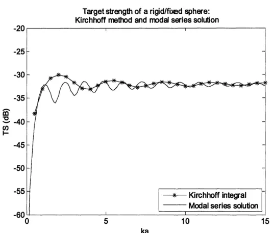
Target strength of a rigid/fied sphere: Kirchhoff method and modal series solution

-LU -25 -30 -35 -40 I---45 -50 -55 -Ai 0 10 ka

Figure 3 - Target strength of a rigid/fixed sphere of radius 5 cm, from the Kirchhoff method (starred line) and modal series solution (smooth line).

Figure 3 shows how the Kirchhoff method result seems to converge to the exact solution as ka increases. However, both curves have strikingly different phases for their peak and null

(30)

patterns. The reason for this is that the Kirchhoff method does not include the effects of diffraction around the sphere. The modal series solution includes both the effects of reflected and diffracted, or creeping, waves. Described by Franz (1957), creeping waves diffract around the object and encircle it multiple times. Watson (1918) and Sommerfeld (1949) described the phenomenon in the study of electric waves diffracting around the Earth. Creeping waves constantly radiate off energy tangentially from the object; some of that radiates in the backwards direction and interferes with the reflected wave. They can be measured

experimentally by using short sound pulses due to their increased travel distance and time (Uberall et al., 1966). These waves can also be influenced by surface waves if the object is elastic. With a rigid/fixed boundary condition, however, they only depend on the geometry of the scatterer. As ka increases and these effects of diffraction lessen, the Kirchhoff method provides a better approximation to the exact modal series solution.

2.4 Scattering from a Finite Cylinder

In this section, the Kirchhoff integral is solved for a rigid/fixed finite cylinder. The results are compared to an approximate modal series based solution for a rigid/fixed finite cylinder. This latter approximation is based on the exact modal series solution for scattering from an infinite cylinder. The approximation neglects the effects of the end of the finite cylinder, and is therefore most accurate near broadside. Therefore, the Kirchhoff integral for the rigid/fixed

finite cylinder is solved so the incident wave is normal to the cylinder's axis.

2.4.1 Kirchhoff Integral Solution for a Finite Cylinder

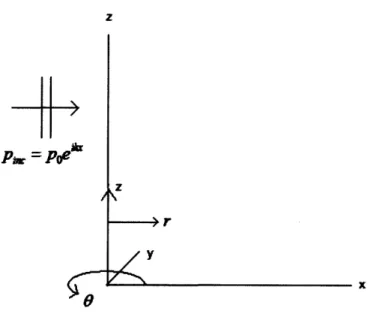
The first step involves defining a cylindrical coordinate system with radial variable r, polar variable 9, vertical variable z, and the same Cartesian coordinate system as was defined in the previous section. Assume the finite cylinder with length L and radius a is centered at the origin so that it is lengthwise along the z axis. An incident plane pi,, = Poei' wave

(31)

traveling in the positive x direction strikes the cylinder normal to its axis. Because the incoming wave arrives at broadside, the cylinder ends are not insonified and therefore do not contribute

to the scattering as calculated using the Kirchhoff integral. Therefore only the sides of the cylinder are considered.

Z

PcW = Poe*

4;

- r

A

Figure 4 - Cylindrical coordinate system, shown with incoming wave and without scatterer geometry.

It can thus be seen that

(2.20)

i = cos 0i + sin 8 i = a cos 09 + a sin 0 + zOi

dao = adOdz .

Substituting these expression into the Kirchhoff integral gives . L/2 3x/2

f = f Cos ei2_kacsOdOdz.

-L/2 r/2

The integral over z is straightforward, leaving

ikaL 3/2

f

= ai cos ei2kacosdO.

1/2

(2.21)

(32)

It is split in order to help solve

kL F r 3r2 1 (2.23)

ikaL cos ei2kacosJd + cos ei2kacosod0I

Two substitutions are made: in the first integral, a = -0 + r; in the second integral, = 8- r :

ikaL -cos ae-i2kacosada + -cos e-i2kacosd

(2.24)

0 0

Both integrals can be solved with help of the relationship (Gaunaurd, 1985)

l'/2 (2.25)

cosxe-iosdx = 1 - [H, (z) + iJ (z)],

f

2

where H, is the Struve function of order one, and J1 is the Bessel function of the first kind of

order one. Thus, equation (2.24) becomes

-ikaL (2.26)

f = [2 - ;[H (2ka) + iJ (2ka)]]. (2.26)

Target strength easily follows from equation (2.11).

2.4.2 Modal Series Based Solution for a Finite Cylinder

The modal series approximation for the scattering of finite cylinders is based on the exact modal series solution for an infinite cylinder. It assumes that end effects are negligible, and, therefore, it is much more accurate near broadside than at high angles of incidence. Stanton

(1988) gives the expression for scattering from a rigid/fixed finite cylinder of length L and radius a: -iL sin A (2.27) f = B,.(-i)" cos(mp) A m=0 where A = kL( - ) - Fc (2.28) 2

(33)

and B, -emimJm'(ka) (2.29) H,'' (ka)

The P terms represent the unit position vectors of the source (subscript i), receiver (subscript r), and cylinder's axis (subscript c). In the case of broadside incidence, A = 0 .The term (p is the angle between the source and receiver vectors in the plane perpendicular to the cylinder axis. For the backscattering case, q7 = ;r, and therefore cos(m~p) = (-1)m. The term 6m is equal to 1 for

m = 0 _{and equal to 2 for all other vales of m . Thus, the backscattering amplitude becomes}

iL e, (-1)" J' (ka) (2.30)

f =

Z m=0 H('l)(ka) Target strength follows from equation (2.11).

(34)

2.4.3 Comparison of Kirchhoff Method and Modal Series Based Solution

for a Rigid/Fixed Finite Cylinder

4r'

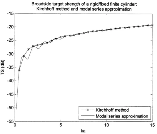
Broadside target strength of a rigid/fixed finite cylinder: Kirchhoff method and modal series approximation

-10 -20 -25 -30 -35 -40 -45 -50 -55 --- Kirchhoff method

- Modal series approximation

ka

Figure 5 - Broadside target strength of a rigid/fixed finite cylinder of length 10 cm and radius 1 cm using the Kirchhoff method (starred line) and modal series approximation (solid line).

As with the sphere, there is a discrepancy in the null-peak phase patterns caused by the creeping waves not accounted for in the Kirchhoff method. The effects of this are again lessened as ka increases. There seems to be much less of an effect from creeping waves for the finite cylinder than for the sphere, as evidenced by the former's better agreement with the Kirchhoff method. It is hypothesized that while the waves diffract relatively well around the entire body of the sphere and the curved sides of the cylinder, they do not diffract as well around the flat ends of the cylinder.

(35)

2.5 Kirchhoff Method Approximations for the Sand Dollar

When an object's geometry becomes too complex, it may not be possible to obtain a closed form solution to the Kirchhoff integral. However, it is possible under some circumstances to approximate the complex geometry of the object with a simpler geometry that does have an analytic solution to the Kirchhoff integral. A sand dollar is an example of a complex geometry where the integral expression cannot be solved analytically due to its irregular shape and surface roughness. Generally, sand dollars have flat bottoms and slightly domed tops in addition to fine scale surface roughness. In this section, the Kirchhoff integral is solved for objects that approximate both of the orientations of the sand dollar. A round disk is used to model the flat bottom and a spherical cap is used to model the rounded top. This section starts with the use of the Kirchhoff integral to derive scattering from an infinitely thin, rigid/fixed disk, as this sheds light on the derivation for the (finite thickness) disk and spherical cap.

2.5.1 Kirchhoff Integral Solution for an Infinitely Thin Disk

The first step in solving the Kirchhoff integral for a disk is to start with the simplest case, a circular rigid/fixed disk of radius a and zero thickness. The lack of thickness means that only the front round face of the disk is incorporated into the solution. Returning to the cylindrical coordinate system, assume the disk is located at the origin, perpendicular to the z axis. The

incoming wave vector k forms an angle 6 with the z axis, varying over the range of angles

(36)

a E--- ;--- -1

I I I I

Ip

Figure 6 - Geometry of the infinitely thin disk.

In this coordinate system, the relevant parameters of the Kirchhoff integral are given by

k =-ksin fl + k cos (2.31)

n = -Z

r = rcos0x + rsin9 O do = rdrd .

Substituting these into the Kirchhoff integral, the backscattering amplitude is given by

-2icosfl (2.32)

-2i fr e -i2krsinc Od

dr .

0 0

Abramowitz and Stegun (1965) give an integral definition of a Bessel function of the first kind:

n ()d(2.33)

J (z)=

e

cos(no)d

Substituting this expression back into equation (2.32), the backscattering amplitude is

a (2.34)

f

2= rJo (-2krsin ,)dr . 0

Next, the substitution z = -2kr sin/i is made

(37)

= -2ricosj -2kasinf -Z J ) - ricos(2.35)-2kasn zJ(z)dz

=

-A o 2ksin fl ) _{2ksinf 2Ak}2_sin

(z) Abramowitz and Stegun give the derivative of a Bessel function as

CI

dp

'P

=

(2.36)

z dz [zJ( = zJ(z).

Setting p = v = 1, this simplifies to

d (2.37)

-[zJ(z)] = zJo(z).

Substituting and solving,

icos -2kasi ()] = (-2ka sin) cos (2.38)

f=2k sinf 0 2sinfc

The target strength of the rigid/fixed, infinitely thin disk is thus given by

TS =10

log I a (-2ka sin fl)cos l2 (2.39)

TS=

0log

.

Urick (1983) gives this result in a slightly different form as the target strength of a circular plate.

2.5.2 Kirchhoff Integral Solution for a Disk with Finite Thickness

The next step in solving the Kirchhoff integral for the disk is to give it a thickness. There are now two different scattering regions of the disk: the flat round face and the curved edge. The height of this new edge is the disk's thickness, T.

(38)

2

a

TI

*

I

...I, ... ..T. K.... K...

k

Figure 7 - Geometry of the disk.

The disk is simply a finite cylinder with an extremely high radius to length aspect ratio. Therefore, this derivation is like that of the finite cylinder over any angle of incidence. The Kirchhoff integral can be split to analyze each of the disk's elements. These two regions of scattering add coherently to give the total scattering amplitude,

f = fface + fedge (2.40)

The backscattering amplitude of the face is very similar to before, with the only difference being a phase shift due to the face's negative displacement by T/2,

ika 2,1 (-2ka sin ,) cos f -ikTcos/ (2.41) 2ka sin f

Next, the scattering from the edge is evaluated. The relevant parameters within the Kirchhoff integral are given by

k= -k sin ,f6 + k cos fi (2.42) n = cos O^ + sin 0F r = a cos 9 + a sin 093 + z do = adOdz. ; ~j ,

(39)

Substituting into the integral expression, the backscattering amplitude is given by

. T/2 /2 (2.43)

fedge = 2

J

-sin

fl

cos9ei2( sina~dos+cos. )ad .dz.

-T/2 -x/2

The integral over z is straightforward:

-ia sin(kT cos

/)

sin

fl

cos e-i2asincdO (2.44)

fedge2 cosd

27r cos/ -fl2-;/2

To solve this integral it first must be split. Then a substitution a = -0 is made in one of the resulting integrals:

fedge

=

-ia sin(kT cos f) sinfl 0 osee.i

2_kinsidcos ₊ ose-i2kas d (2.45)

21 cos/ -2f _-2 _n20f

fedge = -ia sin(kT cos fl) sin cosaeifl 2kasinfcosada+

J

Cose-2asinf' O

(2.4

2rcos/

L

a

These integrals may now be solved with help from equation (2.25), giving

-ia sin(kT cos /) sin

/

(2.47)

fe -ia sin(kT cos ) sin [2 - [H, (2ka sin

/f)

+ iJU (2ka sin fl)]] (2.47).

2 cosp

Gaunaurd (1985) presents a similar derivation and arrives at the same result in his discussion of total insonification of a finite cylinder. The target strength of the rigid/fixed disk is thus given by

TS = 10 log I fac + fedge 12 (2.48)

ika2_{j (-2ka sin}_f)_cos

₃

_e-ikTcos _{ia sin(kT cos}_f)_sin

_/2

= 10log 2ka sinfl 2; cos /

x[2- [H (2ka sin f) + i1 (2ka sin

/)]]

2.5.3 Kirchhoff Integral Solution for a Spherical Cap

The next object that the Kirchhoff integral is solved for is a spherical cap, modeling the sand dollar's top side. Returning to the spherical coordinate system, assume a sphere of radius a centered at the origin. A slice perpendicular to the x-y plane is made through the top half of

(40)

the sphere, and everything below is discarded, leaving only the top cap of the sphere. Another way to define the cap is by polar angle, 0 = 0 to some angle r . The incident wave makes an angle f with the z axis.

z Sk / \B I.

,'V

rX

. '17/

Figure 8 - Geometry of the spherical cap.

The relevant parameters of the Kirchhoff integral are given by

k= -k sin L +kcos fi (2.49)

i = cos ( sin ~O + sin gsin 09 + cos 09

i'= a cos qP sin Ox + a sin (p sin 0 + a cos O2

dr = a2 sin OdOd( . Substituting into the Kirchhoff integral and simplifying,

ika2 _2T_? _(2.50)

f

= - J((sin f cos p sin 9 - cos fl cos ) sin 9ei2ka(sinfscossinO-cosfcosO)dd p.

2r 0

This author is not aware of an analytic solution, so this double integral is to be evaluated numerically.

(41)

2.6 Solving the Kirchhoff Integral Numerically

Using a simplified approximation to the geometry of a complex shape in order to obtain a closed form, analytic solution to the Kirchhoff integral can introduce errors into the predicted scattering associated to the geometric differences. In cases where analytic simplification is impractical, or the resulting errors are unacceptable, it is possible to use a numerical approach to solve the Kirchhoff integral that does not rely on simplifying the object's shape. In this section, a method is presented for solving the Kirchhoff integral numerically, regardless of the object's irregularities.

2.6.1 Creating Geometry and a Mesh in COMSOL Multiphysics

The first step in solving the Kirchhoff integral numerically is to create a surface mesh of the object of interest. This is simply a collection of small connected triangles that attempt to match the surface of the object. The size of these triangles determines how well they conform to the shape. One simple method for creating the object's surface mesh is through use of the finite element software COMSOL Multiphysics@ (ver. 3.2a), referred to in this work simply as

COMSOL. COMSOL is a commercially available program for solving finite element method problems, which will be explored further in Chapter 3. For now, it is used for its capability to model and mesh complex geometries.

Within COMSOL, the geometry of the object of interest can be created using either the GUI or script. Objects can be created from scratch or imported as computer-aided design (CAD) files. Once the geometry is created, a mesh can be generated to conform to it. The mesh for a three dimensional object consists of tetrahedrons in the interior and triangles on the surfaces. The vertices of these shapes are known as mesh vertices. The mesh is created by defining input parameters that regulate the size of the triangles and tetrahedrons and how well they conform to curved parts of the geometry. The size of the triangles on the geometry's surface will have an effect on the accuracy of numerical solution to the integral, since each triangle acts a differential element.

(42)

The mesh may be represented by two sets of information: coordinates and connectivity. The coordinate information lists the location of each of the numbered mesh vertices. The connectivity lists the vertices (by number) that make up each of the mesh elements, in some

systematic way (e.g. counterclockwise for triangles, right hand rule for tetrahedrons). In this way, each mesh tetrahedron is defined by a connectivity of four vertices whose locations are

contained in the coordinate list. Similarly, each triangle is defined by three vertices. Because the Kirchhoff method uses a surface integral, only the information regarding the surface triangles is important. This can easily be separated and assembled within COMSOL into two arrays.

2.6.2 Determination of Insonified Surface

Once the two surface mesh arrays have been compiled, the next step is to determine which triangular surface elements should contribute to the solution. Because the Kirchhoff integral is only applied to the insonified region of the object, any surface in the shadow needs to be ignored. When solving the integral analytically, the proper surface of the object is defined by the limits of integration. Since these are not defined here, there needs to be some way to

eliminate the triangle elements that are not in the line of sight of the incoming wave vector. This problem is similar to one in computer graphics, where several surfaces or polygons share the same set of pixels. In order to display the correct surface (e.g. that which is closest to the viewer), a process known as hidden surface removal determines what information each pixel should display (De Berg et al., 1997). Newell's algorithm is a similar method for determining which polygons are hidden (Newell, 1972). A simplified version of Newell's algorithm is

developed here in order to determine which triangles are hidden by others, from the view-point of the incoming wave vector.

To use the method developed here, a step must be taken before the mesh is created. In order to avoid complicated coordinate transforms later on, the incoming wave vector is set to always coincide with the negative z direction. The object can be rotated in COMSOL so that the desired angle of incidence is achieved. After the mesh is created for this orientation of the object, the simplified version of Newell's algorithm can be applied: