HAL Id: hal-00318028
https://hal.archives-ouvertes.fr/hal-00318028
Submitted on 3 Jul 2006
HAL is a multi-disciplinary open access
archive for the deposit and dissemination of
sci-entific research documents, whether they are
pub-lished or not. The documents may come from
teaching and research institutions in France or
abroad, or from public or private research centers.
L’archive ouverte pluridisciplinaire HAL, est
destinée au dépôt et à la diffusion de documents
scientifiques de niveau recherche, publiés ou non,
émanant des établissements d’enseignement et de
recherche français ou étrangers, des laboratoires
publics ou privés.
Enhanced gravity-wave activity and interhemispheric
coupling during the MaCWAVE/MIDAS northern
summer program 2002
E. Becker, D. C. Fritts
To cite this version:
E. Becker, D. C. Fritts. Enhanced gravity-wave activity and interhemispheric coupling during the
MaCWAVE/MIDAS northern summer program 2002. Annales Geophysicae, European Geosciences
Union, 2006, 24 (4), pp.1175-1188. �hal-00318028�
www.ann-geophys.net/24/1175/2006/ © European Geosciences Union 2006
Annales
Geophysicae
Enhanced gravity-wave activity and interhemispheric coupling
during the MaCWAVE/MIDAS northern summer program 2002
E. Becker1and D. C. Fritts2
1Leibniz-Institute of Atmospheric Physics, K¨uhlungsborn, Germany
2Colorado Research Associates Division, Northwest Research Associates, Boulder, Colorado, USA
Received: 19 July 2005 – Revised: 2 February 2006 – Accepted: 13 Febraury 2006 – Published: 3 July 2006
Part of Special Issue “MaCWAVE: a rocket-lidar-radar program to study the polar mesosphere during summer and winter”
Abstract. We present new sensitivity experiments that link
observed anomalies of the mesosphere and lower thermo-sphere at high latitudes during the MaCWAVE/MIDAS sum-mer program 2002 to enhanced planetary Rossby-wave ac-tivity in the austral winter troposphere.
We employ the same general concept of a GCM having simplified representations of radiative and latent heating as in a previous study by Becker et al. (2004). In the present version, however, the model includes no gravity wave (GW) parameterization. Instead we employ a high vertical and a moderate horizontal resolution in order to describe GW ef-fects explicitly. This is supported by advanced, nonlinear momentum diffusion schemes that allow for a self-consistent generation of inertia and mid-frequency GWs in the lower atmosphere, their vertical propagation into the mesosphere and lower thermosphere, and their subsequent dissipation which is induced by prescribed horizontal and vertical mix-ing lengths as functions of height.
The main anomalies in northern summer 2002 consist of higher temperatures than usual above 82 km, an anomalous eastward mean zonal wind between 70 and 90 km, an al-tered meridional flow, enhanced turbulent dissipation be-low 80 km, and enhanced temperature variations associated with GWs. These signals are all reasonably described by differences between two long-integration perpetual model runs, one with normal July conditions, and another run with modified latent heating in the tropics and Southern Hemisphere to mimic conditions that correspond to the un-usual austral winter 2002. The model response to the en-hanced winter hemisphere Rossby-wave activity has resulted in both an interhemispheric coupling through a downward shift of the GW-driven branch of the residual circulation and an increased GW activity at high summer latitudes. Thus a quantitative explanation of the dynamical state of the
Correspondence to: E. Becker
northern mesosphere and lower thermosphere during June– August 2002 requires an enhanced Lorenz energy cycle and correspondingly enhanced GW sources in the troposphere, which in the model show up in both hemispheres.
Keywords. Meteorology and atmospheric dynamics
(Gen-eral circulation; Middle atmosphere dynamics; Waves and tides)
1 Introduction
The austral winter 2002 was an exceptional season in several respects. The most prominent feature was a major strato-spheric warming observed above Antarctica in mid Septem-ber – the first ever recorded in the southern winter hemi-sphere (Roscoe et al., 2005). This spectacular event trig-gered numerous investigations intended to identify its dy-namical origin, which lies in the preceding temporal evolu-tion of planetary Rossby waves (Harnik et al., 2005). Indeed, when considering the variability of the southern troposphere and stratosphere between June and September 2002, it is ap-parent that the entire season exhibited unusually strong plan-etary Rossby-wave activity (e.g. Baldwin et al., 2003). As a result, the southern polar night jet in 2002 was on average weaker, warmer, and more variable than in other years, to some extent resembling its boreal winter counterpart. Also the rather weak ozone hole in early spring 2002 can be at-tributed to the anomalous dynamics and the late winter major warming (Stolarski et al., 2005).
Coincidently, the MaCWAVE/MIDAS program to study the polar summer middle atmosphere took place in 2002 at the site of Andøya (69.3◦N in northern Norway), per-forming observations of GWs, turbulence, and the mean dy-namical state (Goldberg et al., 2004). Particular empha-sis was placed on the upper mesosphere and lower thermo-sphere (MLT). In comparing the observations from 2002 with
1176 E. Becker and D. C. Fritts: Enhanced gravity-wave activity and interhemispheric coupling
Figure 1: The mean thermal and dynamical structure of the summer MLT at Andøya
in years prior to 2002 (solid curves) and during the MaCWAVE/MIDAS campaign 2002
(dashed curves or dots). (a) Temperature based on falling sphere soundings. (b),(c) Mean
horizontal winds obtained with the ALOMAR MF radar between June 15 and July 15,
2005. (d) Turbulence dissipation rates based on CONE rocket soundings. For details of
the different data sets see Goldberg et al. (2004), Singer et al. (2005), and Rapp et al.
(2004).
26
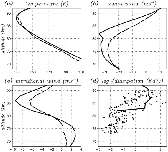
Fig. 1. The mean thermal and dynamical structure of the summer MLT at Andøya in years prior to 2002 (solid curves) and during the
MaCWAVE/MIDAS campaign 2002 (dashed curves or dots). (a) Temperature based on falling sphere soundings. (b), (c) Mean horizontal winds obtained with the ALOMAR MF radar. (d) Turbulence dissipation rates based on CONE rocket soundings. For details of the different data sets see Goldberg et al. (2004), Singer et al. (2005), and Rapp et al. (2004).
those from previous years, systematic anomalies were iden-tified. Figure 1 provides an overview of the major depar-tures noted by Goldberg et al. (2004), Singer et al. (2005), Fritts et al. (2004), and Rapp et al. (2004). From panel (a) we see that the northern summer mesosphere in 2002 was colder than usual by ∼5 K below about 82 km and warmer at higher altitudes (see also Singer et al., 2005, Fig. 2). The observed mean zonal wind was also different from previ-ous years, showing an anomalprevi-ous eastward component be-tween 70 and 90 km (Fig. 1b). An even more striking signal can be seen in the averaged radar observations of the merid-ional wind above Andøya (Fig. 1c). Since standing planetary waves are absent in the extratropical summer middle atmo-sphere according to the Charney-Drazin criterion (see An-drews et al., 1987), we expect the temporal mean temperature and zonal and meridional winds to be good approximations to the temporal zonal means. Therefore, the reduction and downward shift of the equatorward flow in Fig. 1c reflects a
corresponding shift of the zonal-mean drag generated by the breakdown of internal GWs. Assuming that the turbulence in the MLT results primarily from the nonconservative prop-agation of GWs, the downward shift in the meridional wind should be associated with enhanced turbulence at lower al-titudes than usual. Indeed, Rapp et al. (2004) observed sig-nificant turbulence dissipation rates as low as 73 km during the MaCWAVE/MIDAS northern summer program, whereas in previous summers turbulence had never been observed be-low 80 km (L¨ubken et al., 2002). The average dissipation rate prior to 2002 is depicted in Fig. 1d (solid curve) along with the individual soundings from 2002 (dots).
In an earlier study by Becker et al. (2004, B04) an at-tempt was made to relate these exceptional observations in the northern MLT during June–August 2002 to the anoma-lously high planetary Rossby-wave activity in the Southern Hemisphere at the same time. Those authors used a mech-anistic GCM from the surface to 100 km providing explicit
description of planetary and synoptic waves. However, GWs were parameterized according to Lindzen (1981) and Becker (2004), assuming a fixed, horizontally uniform GW source at 170 hPa. The mechanistic character of the model was due to its thermal forcing, using temperature relaxation to mimic radiative heating, prescribed tropical heating to represent the cumulus convection zones along the equator, and self-induced condensational heating in middle latitudes (K¨ornich et al., 2003). The strength of this simplicity lies in the possi-bility to adjust the latent heating functions in order to realize different states of planetary Rossby-wave activity in perpet-ual long-integration simulations.
Taking advantage of this utility, B04 performed two sim-ulations, one with “normal July” conditions and a sensitivity experiment with “July 2002” conditions. The general con-clusion drawn by comparing the climatologies of both runs was that the aforementioned anomalous observations in the northern summer MLT can qualitatively be interpreted as the interhemispheric coupling communicated by a downward shift of the GW-driven summer-to-winter-pole residual cir-culation. In particular, enhanced Rossby-wave activity in the winter stratosphere leads to a weaker and more variable polar night jet, which in turn causes the saturation levels of GWs to shift to lower altitudes and to be distributed over a deeper height range (Becker and Schmitz, 2003). The associated weakening and downward shift of the GW-driven branch of the residual circulation in the winter hemisphere is accompa-nied by a corresponding shift in summer. This shift in sum-mer can only exist in climatological equilibrium if the GW drag shifts downward as well, requiring enhanced eastward flow in the MLT, as observed (Fig. 1b). The associated tem-perature signal is also consistent with this argument, since a downward shift in GW drag implies enhanced adiabatic cooling in the lower part of the MLT and reduced adiabatic cooling above. Here we have ignored the direct thermody-namic effects associated with GW breakdown, which in the GW parameterization used in B04 were dominated by ver-tical mixing of entropy, causing strong cooling in the MLT and weak heating below the breaking levels (Becker, 2004). Hence the response of the direct thermodynamic effects to a downward shift in GW saturation added to the anomalous adiabatic heating. This interpretation by B04 applies at most qualitatively to the anomalous observations in the northern summer MLT during the MaCWAVE/MIDAS campaign.
There are, of course, many obvious reasons why one should not expect any quantitative agreement between the observations and mechanistic model estimates. For exam-ple, statistical significance tests for the differences in the observed dissipation rates are not possible due to the small amount of data. Also, the differences in the temperature pro-files were obtained from only a limited number of sound-ings during 2002, leaving room for uncertainties. On the other hand, the SABER temperature retrievals reported by Goldberg et al. (2006) confirm lower temperatures than usual below 80 km for northern summer 2002 when compared to
2003 or 2004, and they support higher temperatures farther above for at least the difference between the 2002 and 2003 northern summer seasons. Furthermore, the more nearly con-tinuous radar measurements of meridional and zonal winds may be considered to be robust.
Concerning the model, the simplistic thermal forcing is questionable with regard to both the troposphere and the mid-dle atmosphere, but may be acceptable in order to reveal the dynamical mechanism. The major uncertainty in the B04 model, however, lies in the strong assumptions that consti-tute a GW parameterization. Despite single-column-GW dy-namics, an instantaneous response of the whole GW column to any change in the resolved flow, and the general uncer-tainty in the details of the dissipation mechanism (McLan-dress and Scinocca, 2005), GW parameterizations generally suffer from the fact that GW sources must be tuned in such a way to make the model behave reasonably. Attempts to re-late the GW sources to the dynamics of the resolved scales (Charron and Manzini, 2002) may be considered as a first step to reduce the ambiguity of assumed GW sources in GW parameterizations.
GW temperature variances observed at Andøya during summer 2002 indicate that either 1) GW sources in the lower atmosphere were extraordinaryly strong or 2) propa-gation conditions enabled large-amplitude GWs in the MLT (Fritts et al., 2004; Rapp et al., 2004). Large energy dissipa-tion rates and turbulence at lower altitudes than previously observed also support this hypothesis (Rapp et al., 2004; Fig. 1d). Therefore, a downward shift in the GW-driven residual circulation induced by interhemispheric coupling is probably not the full story to the observations during the MaCWAVE/MIDAS campaign. A more thorough interpreta-tion on the basis of GCM experiments requires us to account for both the interhemispheric coupling and possible anoma-lies of the GW sources.
The purpose of this study is to present an expanded in-terpretation of the anomalous dynamics in northern summer 2002 based on more complete GCM simulations. The ma-jor difference from the model configuration used by B04 is that we now dispense with a GW parameterization and sim-ulate GW effects explicitly. Such an attempt is not new (e.g. Hamilton et al., 1995, 1999). In accordance with arguments by Lindzen and Fox-Rabinovitz (1989), the present model configuration employs a high vertical resolution (190 hy-brid levels) in order to adequately describe the propagation of GWs up to the lower thermosphere. The spectral reso-lution is T85. Obviously, such a model cannot in any way represent all GW scales known to be relevant in the MLT re-gion (Fritts and Alexander, 2003). Especially high-frequency GWs are excluded. On the other hand, such a model setup can capture well the generation and propagation of inertia GWs and mid-frequency GWs, with the latter transporting sufficient momentum from low to high altitudes to account for considerable zonal-mean GW dissipation and drag in the MLT. It is likely that the resolved GW drag would occur at
1178 E. Becker and D. C. Fritts: Enhanced gravity-wave activity and interhemispheric coupling
Figure 2: Prescribed fields used for thermal forcing in the simple GCM. (a),(b)
Equilib-rium temperature T
e(contour interval 20 K) and corresponding thermally balanced zonal
flow U
e(contour interval 20 ms
−1). (c),(d) Horizontal structure of the heating functions in
the ’normal July’ run (black contours for 1, 2, 3 Kd
−1) and in the ’July 2002’ run (white
contours for 1, 2, 3 Kd
−1) at different pressure levels. (e) Same as (c),(d), but for the
surface temperature (contour interval 20 K). (f) Same as (c),(d), but for the zonal means
in a latitude-height cross-section (contour interval 0.5 Kd
−1).
27
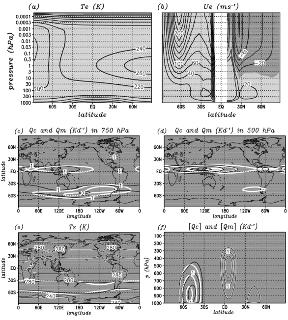
Fig. 2. Prescribed fields used for thermal forcing in the simple GCM. (a), (b) Equilibrium temperature Te (contour interval 20 K) and
corresponding thermally balanced zonal flow Ue(contour interval 20 ms−1). (c), (d) Horizontal structure of the heating functions in the
“normal July” run (black contours for 1, 2, 3 Kd−1) and in the “July 2002” run (white contours for 1, 2, 3 Kd−1) at different pressure levels.
(e) Same as (c),(d), but for the surface temperature (contour interval 20 K). (f) Same as (c), (d), but for the zonal means in a latitude-height
cross-section (contour interval 0.5 Kd−1).
shorter horizontal wavelengths and higher intrinsic frequen-cies if higher horizontal resolution was employed, and this question deserves to be addressed in the future. Nonetheless, the present model setup enables tropospheric GW sources to be simulated in a self-consistent manner, offering the oppor-tunity to address the question raised by the findings of Fritts et al. (2004) and Rapp et al. (2004), namely whether en-hanced tropospheric GW forcing may have contributed to the extraordinary dynamical state of the northern summer MLT in 2002.
The outline of this paper is as follows. In the next sec-tion we describe those aspects of the present GCM that are of particular importance for the purpose of the present study. In Sect. 3 we compare the climatologies of the new sensitiv-ity experiments, which were performed using essentially the same thermal forcing as in B04. Section 4 analyzes changes in the northern tropospheric GW sources that are induced by changing the latent heating functions in the southern and tropical troposphere. We briefly discuss anomalies of the temperature variations in Sect. 5. Section 6 presents re-sults from a “transient” experiment in which we continuously
Figure 3: Assumed vertical profiles of (a) the asymptotic vertical mixing length and (b)
the horizontal mixing length.
28
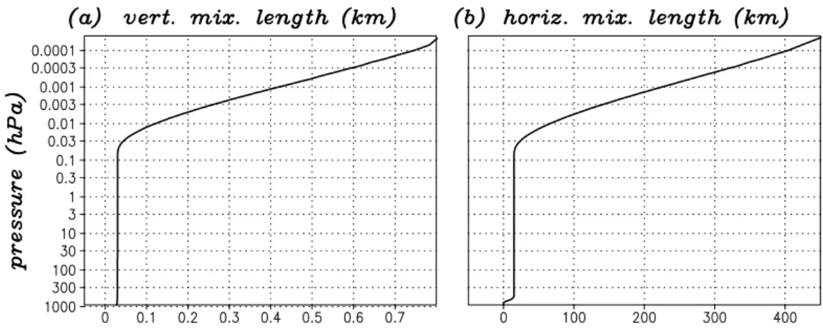
Fig. 3. Assumed vertical profiles of (a) the asymptotic vertical mixing length and (b) the horizontal mixing length.
simulate the transition from the assumed “normal July” to the “July 2002” conditions. This experiment is designed to re-visit and interpret the character of the interhemispheric cou-pling by the summer-to-winter-pole residual circulation. In this context we also estimate the typical time scale of the interhemispheric coupling. Our results are summarized in Sect. 7.
2 Model description
Our model is the K¨uhlungsborn Mechanistic general Circula-tion Model (KMCM). This simple GCM has a standard spec-tral dynamical core. In its present setup we adopt 190 full hybrid levels from 0.1 to about 125 km, resulting in a verti-cal level spacing of approximately 550 m from the boundary layer to 100 km. Due to the restriction of computer resources we have run a horizontal resolution of T85 corresponding to a horizontal gridspacing of 1.4 deg or 162 km. We abbrevi-ate this model version as T85/L190 model. The former low-resolution simulations presented in B04 were performed with the T31/L60 version.
We apply permanent July conditions and there is no forc-ing of thermal tides. The total diabatic heatforc-ing in terms of sensible heat per unit mass divided by heat capacity cpcan
be written as Q = −T − Te
τ +Qc +|ω| h(−ω)
40 mb d−1Qm
+diffusion + frictional heating . (1) As usual, T is temperature and Tea zonally symmetric
equi-librium temperature which is displayed in Fig. 2a. The corre-sponding thermally-balanced zonal mean wind is shown for reference in Fig. 2b. The relaxation time τ is 14 days in the troposphere and 7 days in the upper stratosphere and meso-sphere, with an intermediate maximum of 40 days around 100 hPa. The spatial structures of the heating functions Qc
and Qmare displayed in Figs. 2c, d, and f, with black
con-tours corresponding to “normal July” conditions and white contours to “July 2002” conditions. The surface sensible heat flux is computed from a local boundary layer scheme (Holtslag and Boville, 1993) with the surface temperature (see Fig. 2e) defined as
Ts = [Te+0.4 τ Qc+Qm) ]surface. (2)
The differences in thermal forcing between the two model experiments are designed to induce enhanced planetary Rossby-wave activity in the Southern Hemisphere in the “July 2002” simulation. This aim is achieved by assuming al-most the same heating functions for “normal July” and “July 2002” as in B04 – despite an additional self-induced heating over the continents in the northern extratropics, where the heating function Qmis identical in both simulations. Note
that the Qc maximum over the maritime continent is shifted
somewhat into the tropical Pacific in the “July 2002” exper-iment in order to account for the El Nin´o in 2002. Such a procedure follows the method of Ting and Held (1990) and has turned out to be necessary for stronger planetary Rossby waves in the Southern Hemisphere in our “July 2002” simu-lation. Our second aim to also describe a possibly enhanced GW forcing in the northern summer troposphere for 2002 conditions is not controlled by any specified change in model forcing, but is instead allowed to respond to other shifts in lo-cal conditions such as an anomalous stationary Rossby-wave train that is induced by the modified Qcand ranges from the
western tropical Pacific over North America to the North At-lantic (Ting and Held, 1990).
KMCM employs special parameterizations of turbulent friction. First, horizontal diffusion is included using a gener-alized mixing length approach in association with a symmet-ric stress tensor formulation appropriate for sphesymmet-rical coor-dinates (Smagorinsky, 1993; Becker, 2001). The details are
1180 E. Becker and D. C. Fritts: Enhanced gravity-wave activity and interhemispheric coupling
Figure 4: Zonal-mean climatology for ’July 2002’ conditions. (a) Temperature (contour
interval 20 K). (b) Zonal wind (contour interval 20 ms
−1). (c) Eulerian meridional wind
(contour interval 2 ms
−1). (d) Dissipation (contours 0.25, 0.5, 1, 2, 4, 6, 8 Kd
−1). Zero
contours are not drawn. Positive and negative values are indicated by light and dark
shading. The additional white contours in (c) show the residual mass streamfunction
Ψ
res(contours ±0.01, 0.1, 1, 10, 100 × 10
9
kgs
−1).
29
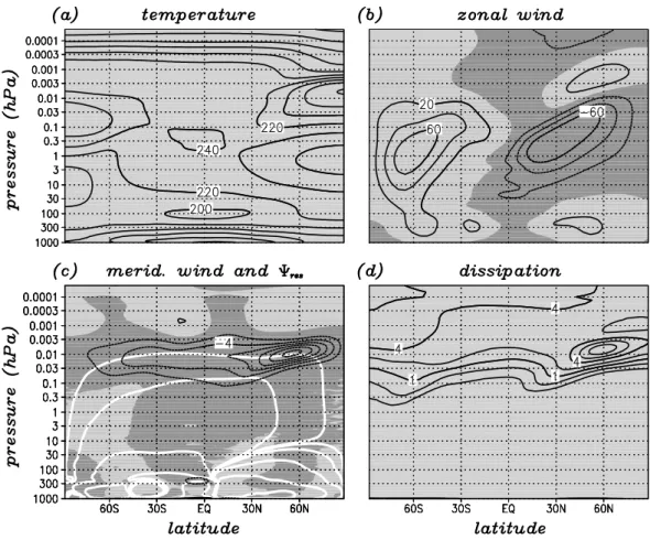
Fig. 4. Zonal-mean climatology for “July 2002” conditions. (a) Temperature (contour interval 20 K). (b) Zonal wind (contour interval
20 ms−1). (c) Eulerian meridional wind (contour interval 2 ms−1). (d) Dissipation (contours 0.25, 0.5, 1, 2, 4, 6, 8 Kd−1). Zero contours are not drawn. Positive and negative values are indicated by light and dark shading. The additional white contours in (c) show the residual mass streamfunction 9res(contours ±0.01, 0.1, 1, 10, 100×109kgs−1).
given in Becker and Burkhardt (2006)1. In short, the hori-zontal diffusion coefficient is written as Kh=lh2|S|, where lh
denotes the horizontal mixing length and √
2 |S|is the Frobe-nius norm of the strain tensorS. This scheme is better moti-vated physically than conventional hyperdiffusion schemes. It also enables an efficient scale selectivity and satisfies all hydrodynamic conservation laws, including a consistent rep-resentation of the frictional heating (dissipation).
Second, the boundary-layer formulation of the vertical dif-fusion coefficient, which is given by the local scheme de-scribed in Holtslag and Boville (1993), is applied at all model layers, with the asymptotic vertical mixing length prescribed as a function of height. As usual, the upper boundary condi-tions assume zero vertical fluxes at the model lid, and con-ventional flux boundary conditions are applied at the bottom. The molecular diffusion coefficient diffuses momentum, but cpT instead of cp2with respect to sensible heat, where 2
1Becker, E. and Burkhardt, U.: Nonlinear horizontal diffusion
for GCMs. Mon. Wea. Rev., submitted, 2006.
is potential temperature. To calculate the frictional heat-ing associated with vertical momentum diffusion, the finite-differencing method of Becker (2003) is implemented, which explicitly accounts for the no-slip condition in order to en-sure a closed Lorenz energy cycle in the troposphere.
Figure 3 shows the assumed profiles for the asymptotic vertical and horizontal mixing lengths. These profiles were chosen such that the resolved GWs are damped in the MLT. That is, we conceive of a dynamical-convective instability process by which the waves dissolve into smaller-scale waves and finally into turbulence, giving rise to Eliassen-Palm flux divergence that drives the mean flow. Such an assumption is supported by recent direct numerical simulations (Fritts et al., 2003, 2006), but these dynamics are not sufficiently un-derstood for parameterization purposes at this stage. Thus, we must employ an empirical adjustment of diffusion pa-rameters in order to ensure application of the GW drag well below the model upper boundary, as is common in middle-atmosphere GCMs. Advantages of this procedure are 1) no tunable GW parameters occur in the present model and
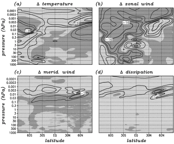
Figure 5: Simulated zonal-mean differences in the ’July 2002’ simulation from the
’nor-mal July’ run. (a) Temperature (contours ±2, 4, 8, 16, 32 K). (b) Zonal wind (contours
±2, 4, 8, 16 ms
−1). (c) Eulerian meridional wind (contours ±1, 2 ms
−1). (d) Dissipation
(contours ±0.5, 1, 2 Kd
−1). Zero contours are not drawn. Positive and negative values are
indicated by light and dark shading.
30
Fig. 5. Simulated zonal-mean differences in the “July 2002” simulation from the “normal July” run. (a) Temperature (contours
±2, 4, 8, 16, 32 K). (b) Zonal wind (contours ±2, 4, 8, 16 ms−1). (c) Eulerian meridional wind (contours ±1, 2 ms−1). (d) Dissipation (contours ±0.5, 1, 2 Kd−1). Zero contours are not drawn. Positive and negative values are indicated by light and dark shading.
2) negligible sponge-layer feedback (Shepherd et al., 1996) in our application.
The time step was 24 s. The “normal July” and “July 2002” experiments were integrated for 200 model days in each case after equilibration of the model climatologies. Model data were sampled every 90 min.
3 Climatologies
Zonal-mean fields for the “July 2002” simulation are shown in Fig. 4. The corresponding differences from the run with “normal July” conditions are displayed in Fig. 5. We will refer to such differences between the two simulations as anomalies, signals, or model response. The simulated zonal-mean general circulation (Fig. 4) is reasonable. However, a few shortcomings due to dispensing with a GW parame-terization should be mentioned. The resolved winter hemi-spheric Eliassen-Palm flux (EPF) divergence (see Appendix) is obviously too weak to account for a wind reversal in the MLT. Also, the resolved wave drag in summer (not shown) is weaker than that provided by a GW parameterization.
Fur-thermore, the assumed equilibrium temperature Te is too
warm by about 10 deg in this region. As a result, the sim-ulated summer mesopause is much warmer than observed. Despite these discrepancies, the simulated dissipation (fric-tional heating) shows the well-known summer-winter asym-metry in the MLT and is much more pronounced at high lat-itudes than in the T31/L60 model, with a shift to higher alti-tudes in summer towards the pole.
The zonal-mean model response (Fig. 5) is generally con-sistent with the previous sensitivity experiments (see B04, their Fig. 5). In particular, the general character of the anomalous temperatures, mean winds, and dissipation rates summarized in Fig. 1 is reproduced by the present T85/L190 model. The signals maximize at high summer latitudes, whereas the T31/L60 model version with parameterized GWs showed almost no sensitivity at high summer latitudes with respect to the meridional wind or the dissipation. That same discrepancy between the old and new simulations is also reflected in the momentum budget as discussed below.
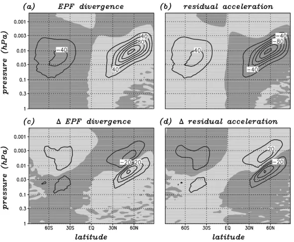
Figures 6a and b show the Eliassen-Palm flux (EPF) di-vergence and the Coriolis force plus nonlinear advection as-sociated with the residual circulation, loosely abbreviated as
1182 E. Becker and D. C. Fritts: Enhanced gravity-wave activity and interhemispheric coupling
Figure 6: Zonal-mean momentum budget in the residual picture. (a) Eliassen-Palm flux (EPF) divergence and (b) Coriolis force plus nonlinear advection associated with the residual circulation in the ’July 2002’ simulation (contour interval 20 ms−1d−1). (c),(d)
Same as (a),(b), but for the difference from the ’normal July’ run (contour interval 10 ms−1d−1). Zero contours are not drawn. Positive and negative values are indicated by
light and dark shading.
31
Fig. 6. Zonal-mean momentum budget in the residual picture. (a) Eliassen-Palm flux (EPF) divergence and (b) Coriolis force plus nonlinear
advection associated with the residual circulation in the “July 2002” simulation (contour interval 20 ms−1d−1). (c),(d) Same as (a), (b), but for the difference from the “normal July” run (contour interval 10 ms−1d−1). Zero contours are not drawn. Positive and negative values are indicated by light and dark shading.
“residual acceleration”, in the “July 2002” experiment. The definitions are given in the Appendix. The sum of the two terms is approximately zero, as should be the case. In partic-ular, the frictional forces associated with our mixing-length sponge layer are negligible. Also the differences in the “July 2002” run from the “normal July” run show a satisfactory balance between the anomalous EPF divergence (Fig. 6c) and the anomalous acceleration by the residual circulation (Fig. 6d), indicating that a sponge-layer feedback (Shepherd et al., 1996) is not relevant in the present model.
Due to the enhanced planetary Rossby-wave activity, there is an anomalous deceleration in the winter stratopause region (Fig. 6c). According to Becker and Schmitz (2003), this should lead to a downward shift of the winter-hemispheric GW drag or, equivalently, to reduced deceleration at higher altitudes where the EPF divergence is dominated by the GW drag. This effect is indeed visible in Fig. 6c above about 0.02 hPa in the southern winter MLT. However, the strongest signal of the anomalous EPF divergence appears in the po-lar summer MLT, where we can infer a highly significant downward shift of the total EPF divergence, with the
anoma-lies being about one third as strong as the absolute values. In this context, we note that the resolved GW drag in the summer MLT is to a significant extent counterbalanced by the deceleration associated with travelling planetary waves which develop in situ as a result of baroclinicity (Lieberman, 1999, 2002). As a result, in each of our two simulations the maximum GW drag is about 30 ms−1d−1stronger than the maximum EPF divergence. On the other hand, the difference of the EPF divergence between both runs is quite similar to the difference of the GW drag (not shown). Since such a pronounced sensitivity of the wave driving at high summer latitudes was absent in the T31/L60 model, we expect that a stronger GW source in the lower atmosphere is essential for the anomalous wave effects in the MLT. In the following section we inspect the anomalous GW sources in more detail.
4 Enhanced gravity-wave activity
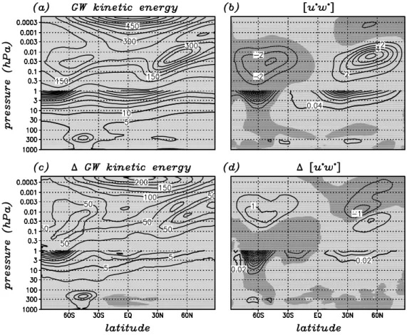
Figures 7a and b show the kinetic energy per unit mass as-sociated with the transient, divergent part of the resolved
Fig. 7. GW kinetic energies and zonal-mean momentum fluxes in the climatological zonal mean. (a) Kinetic energy associated with the
divergent, transient part of the resolved flow in the “July 2002” run (contour interval 50 m2s−2above 1 hPa and 5 m2s−2below). (b) Vertical momentum flux due to transient waves in the “July 2002” run (contour interval 1 m2s−2above 1 hPa and 0.04 m2s−2below). (c),(d) Same as (a), (b), but for the differences in the “July 2002” experiment from the “normal July” simulation (contour intervals are 25 and 0.5 m2s−2 above 1 hPa, or 2.5 and 0.02 m2s−2below). Zero contours are not drawn. Positive and negative values are indicated by light and dark shading.
flow and the vertical flux of zonal momentum associated with transient eddies in the “July 2002” experiment. Apart from synoptic-scale ageostrophic components in the tropo-sphere and winter stratotropo-sphere, we can take these quantities as measures of the resolved GW kinetic energy and resolved GW momentum flux. Accordingly, the extratropical maxima between 0.1 and 0.003 hPa in panels a and b mark the gions of maximum GW-mean flow interaction. Figure 7c re-veals that for “July 2002” conditions the GW kinetic energy is larger everywhere in the middle atmosphere than in the “normal July” case. When we consider the 0.03 hPa level, above which the GW drag sets in, we infer a strengthening of the GW kinetic energy by about 25% poleward of ∼60◦N.
The corresponding increase of the GW momentum flux at polar summer latitudes is about 15%. These intensifications likely contribute to the downward shifts of wave drag, merid-ional wind, and dissipation around 60◦N (Figs. 6c, 5c, and 5d).
The self-induced condensational heating in the Northern Hemisphere is included in the model to describe the large-scale diabatic heating pattern in the northern summer tropo-sphere as diagnosed by Wang and Ting (1999) from observa-tional analyzes. However, even our simple parameterization for latent heating induces the generation of GWs. In fact, neglecting the summer hemispheric Qm results in a
reduc-tion of the mesospheric GW drag by about 50% (not shown). In order not to prescribe any changes in GW sources in the Northern Hemisphere, the corresponding part of the heating function Qm is identical in all our simulations (see Fig. 2).
Furthermore, we have checked that the zonally-averaged and vertically-integrated self-induced condensational heating in the Northern Hemisphere is essentially the same for both the “normal July” and the “July 2002” simulations. Neverthe-less, we can diagnose an enhanced Lorenz energy cycle in the “July 2002” run, with the global-mean dissipation rate being 2.29 Wm−2 compared to 1.84 Wm−2 in the “normal July” run. While this globally-enhanced dissipation is due
1184 E. Becker and D. C. Fritts: Enhanced gravity-wave activity and interhemispheric coupling
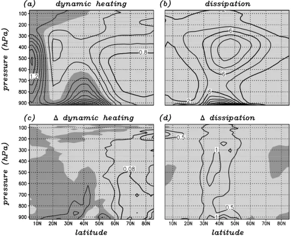
Figure 8: (a),(b) Dynamic heating (adiabatic heating plus advection) and dissipation (frictional heating) in the northern troposphere for the ’July 2002’ simulation. (c)(d) Corresponding differences from the ’normal July’ run. Contour intervals are: (a) 0.2 Kd−1, (b) 2 × 10⁻³ Kd−1, (d) 0.04 Kd−1, (e) 0.5 × 10⁻³ Kd−1. Zero contours are not
drawn. Positive and negative values are indicated by light and dark shading.
33
Fig. 8. (a),(b) Dynamic heating (adiabatic heating plus advection) and dissipation (frictional heating) in the northern troposphere for the “July
2002” simulation. (c), (d) Corresponding differences from the “normal July” run. Contour intervals are: (a) 0.2 Kd−1, (b) 2×10⁻³Kd−1, (d) 0.04 Kd−1, (e) 0.5×10⁻³Kd−1. Zero contours are not drawn. Positive and negative values are indicated by light and dark shading.
primarily to the modified dynamics in the southern tropo-sphere, the northern troposphere also indicates an enhanced energy cycle. Figure 8 shows the dynamic heating, defined as adiabatic heating plus advection by the resolved flow, and the dissipation in the northern troposphere for the “July 2002” simulation, as well as the differences from the “nor-mal July” simulation. Panel (c) clearly indicates enhanced heat transport from low to high latitudes. Furthermore, there is enhanced frictional heating in the mid-latitude troposphere (Fig. 8d), indicating enhanced dissipation of synoptic-scale wave kinetic energy in that region. We have not shown the boundary-layer dissipation below 900 hPa in Fig. 8 since this heating is much stronger than the dissipation in the upper tro-posphere (Becker, 2003) and almost identical in both simula-tions. Summarizing, the enhanced GW activity in the north-ern summer hemisphere for 2002 conditions can be linked to a stronger Lorenz energy cycle in the troposphere. This sensitivity is induced primarily through imposed changes in tropical heating Qcand, probably to a smaller degree, by the
modified winter troposphere. It is beyond the scope of this study to address the causes or the true magnitudes of these effects in greater detail, since our primary focus is on the
summer MLT and we have employed a GCM unable to de-scribe smaller-scale GWs and their energy and momentum transport explicitly.
5 Temperature variances
Figures 9a and b show the zonal averages of the standard deviation of temperature associated with GWs and the corre-sponding relative temperature variance for the model output at 70◦N, which corresponds approximately to the latitude of Andøya. We have chosen to plot zonally averaged variations instead of those at a particular longitude since longitudinal variations in GW effects in the summer MLT are less likely than in winter and the zonally averaged model response is thus more robust. The temperature variations in the sim-ulated summer MLT are generally dominated by travelling planetary waves with zonal wavenumbers m=1 . . . 6, espe-cially the quasi-2-day wave with m=3. Accordingly, the sim-ulated GW variations shown in Fig. 9 have been diagnosed by retaining only zonal wave numbers in excess of m=10. Ob-served temperature variances associated with GWs already presented by Rapp et al. (2004, their Fig. 3) are also included
Figure 9: (a) Zonal mean of the temperature standard deviation at 70oN in the ’normal
July’ run (solid curve) and in the ’July 2002’ run (dashed curve). Only zonal wavenumbers m = 11 . . . 85 are retained. (b) Black curves: Same as (a), but for the relative temperature variation. In addition, the red curves give observed relative temperature variations already presented by Rapp et al. (2004), which were compiled from soundings during years before 2002 (solid curve) and during the MaCWAVE year 2002 (dashed curve).
34
Fig. 9. (a) Zonal mean of the temperature standard deviation at 70◦N in the “normal July” run (solid curve) and in the “July 2002” run (dashed curve). Only zonal wavenumbers m=11 . . . 85 are retained. (b) Black curves: Same as (a), but for the relative temperature variation. In addition, the red curves give observed relative temperature variations already presented by Rapp et al. (2004), which were compiled from soundings during years before 2002 (solid curve) and during the MaCWAVE year 2002 (dashed curve).
in Fig. 9b for the same altitude range (red curves). Differ-ences between the simulated and observed temperature vari-ations may result from insufficient spatial resolution of the model, application of adhoc assumptions in the turbulent dif-fusion schemes, and from uncertainties in the extraction of observed GW variations. Despite these deficiencies, the ob-served intensification of temperature variations is reproduced in our sensitivity experiments quite reasonably.
Rapp et al. (2004) interpreted this signal as a result of an associated increase in the background Brunt-V¨ais¨al¨a fre-quency squared, N2, arguing that the temperature vari-ance of a single GW scales with N2 in regions of sat-uration. The complete dependence, based on the polar-ization relations given in Becker (2004), yields that the relative temperature variance of a saturated GW scales like T02/ ¯T2≈202,/ ¯22∝N2(c− ¯u)2, where c is the phase
speed and ¯uthe horizontal background wind in the direction of propagation.2 In northern summer 2002, N2 was indeed unusually strong due to the modified mean temperature, but at the same time (c− ¯u)2should have been weaker due to the anomalous eastward wind component, provided we assume that only GWs with eastward phase speeds of the order of 30 ms−1are relevant in the summer MLT.
The present numerical experiments clearly support en-hanced GW sources as an explanation of the higher temper-ature variances in the MLT. However, the changes in static stability are not simulated in a satisfactory way, mainly be-cause the absolute model temperatures are too high in the summer MLT by about 30 degrees. Therefore, the origin of the changes in temperature fluctuations cannot be addressed at present. We speculate, however, that the increases in both static stability and GW source strength likely played roles
2The remaining factors consist of constants like the horizontal
wavenumber and the momentum flux at the source level.
in the enhanced temperature variances observed by Rapp et al. (2004) and Fritts et al. (2004) during polar summer in 2002.
6 Interhemispheric coupling in the MLT by the residual circulation
In the winter middle atmosphere, the downward shift of GW drag and the GW-driven branch of the residual circulation is controlled by enhanced planetary Rossby-wave activity in the stratosphere. In particular, stronger planetary Rossby waves induce a weaker and more variable eastward zonal flow, which causes the GW drag to be spread over a deeper height range and to occur on average at lower altitudes. This mechanism has proven to be valid if GW damping is defined via a saturation assumption (Becker and Schmitz, 2003). Ob-viously, it also applies in the present case of mixing-length based horizontal and vertical diffusion schemes (Fig. 6c). The question not answered in previous papers by Becker and Schmitz (2003) or B04 is how this signal is communicated to the summer mesosphere, where a downward shift of GW effects and the residual circulation is also found, even in the case of fixed GW sources. In particular, if we applied the same argument valid for the winter mesosphere to the sum-mer MLT, the downshift in GW drag would suggest a re-duced westward jet in the summer stratosphere and lower mesosphere, rather than stronger westward winds as seen in the previous sensitivity experiments (see B04, their Fig. 5b; Becker and Schmitz, 2003, their Fig. 3) or in falling-sphere wind soundings (Goldberg et al., 2004). Therefore, putting changes in GW sources aside, an explanation of the down-ward shift of the residual circulation in summer must be quite different from that for winter. In the following we propose
1186 E. Becker and D. C. Fritts: Enhanced gravity-wave activity and interhemispheric coupling
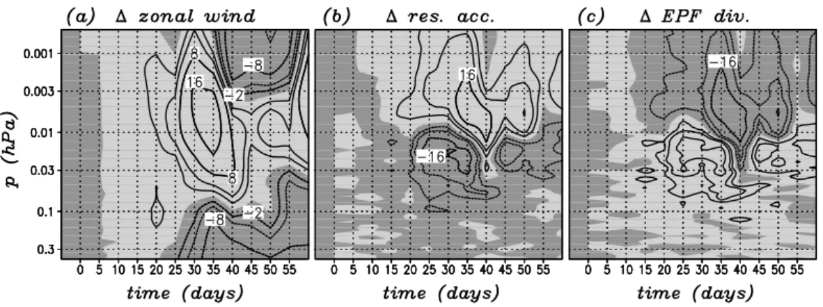
Figure 10: Transient model response with respect to (a) zonal-mean zonal wind (contours ±2, 4, 8, 16 ms−1), (b) residual acceleration (contours ±4, 8, 16 ms−1d−1), and (c) EPF
divergence (contours ±4, 8, 16 ms−1d−1). Each quantity is averaged over 5 days and from
15oN to 60oN. Positive and negative values are indicated by light and dark shading.
35
Fig. 10. Transient model response with respect to (a) zonal-mean zonal wind (contours ±2, 4, 8, 16 ms−1), (b) residual acceleration (contours
±4, 8, 16 ms−1d−1), and (c) EPF divergence (contours ±4, 8, 16 ms−1d−1). Each quantity is averaged over 5 days and from 15◦N to 60◦N. Positive and negative values are indicated by light and dark shading.
an explanation for how the interhemispheric coupling in the MLT might come about.
We argue, for reasons of continuity, that a downward shift of the GW-driven branch of the winter-hemisphere resid-ual circulation will also cause the meridional flow across the equator and in the summer hemisphere to shift to lower altitudes, with the signal decreasing towards the summer pole. This downward shift of the summer hemispheric f vres
corresponds to a net zonal force with acceleration around the altitude of maximum GW drag and deceleration below. The resulting additional eastward wind component will cause in-creased vertical wavenumbers of the eastward propagating GWs, leading to GW dissipation at somewhat lower alti-tudes, which in turn alters the GW drag and the mean zonal flow in a way to balance the altered f vres and maintain
steady downward control.
This transition process can be simulated in the following way. We change the latent heating functions continuously from “normal July” to “July 2002” conditions within one month, starting from some time step in the “normal July” run, defined as day 0. From day 30 on, the “July 2002” heating functions are again constant in the transient experiment. The time series of the transient run are then compared to the cor-responding time series of the “normal July” integration. We monitor subsequent 5-day averages of the zonal-mean zonal wind, the residual acceleration, and the EPF divergence (see Appendix). Figure 10 shows the corresponding differences between the transition experiment and the “normal July” run, averaged between 15◦and 60◦N. The temporal evolution of
the zonal wind signal is evident from panel (a). Note that the positive zonal wind anomaly extends well into the mid-dle mesosphere due to the contribution from low summer latitudes (see Fig. 5b). Comparing panels a and b we see that only the upper half of the positive wind anomaly fol-lows the anomalous residual acceleration (or f vres). Hence,
the transient change of the EPF divergence (or the GW drag)
causes the positive wind anomaly to extend to lower alti-tudes than the transient change in the residual acceleration would suggest. From day 20 or so on, the transient anomalies are contaminated by the independent internal variabilities in the “normal July” and the transient experiments. In particu-lar, the eastward GW momentum flux in the lower summer mesosphere is stronger in the transient run than in the “nor-mal July” run around day 25, but it is weaker around day 40 (not shown). Averaging both runs from day 0 to day 60, the transient intensification of the eastward momentum flux in the summer mesosphere turns out to be about half as strong than the climatological result presented in Fig. 7d. Thus our transient experiment cannot fully isolate the interhemispheric coupling.
Since the interhemispheric coupling occurs not only in sensitivity experiments, but also shows up as a mode of in-ternal variability (Volodin and Schmitz, 2001), a statistical estimate of its typical time scale can be obtained from time-lagged correlations in the “July 2002” simulation. The vari-ations of the daily averaged zonal-mean temperature in the “July 2002” simulation maximize around 55oS, 0.05 hPa and above the summer pole around 0.002 hPa (not shown). These locations correspond to the negative and positive extrema of the temperature signal in Fig. 5a which reflect the global downshift of the summer-to-winter-pole residual circulation. We compute correlations between the time series of daily av-eraged zonal-mean temperatures at the two locations. The re-sulting correlation coefficient minimizes at –0.71 for a time lag of 28 days and it reduces to –0.14 for a 40-day time lag, or to 0.01 for a 10-day time lag. Hence, the typical time scale for interhemispheric coupling in the MLT due to inter-nal variability of planetary Rossby waves in the winter hemi-sphere is about one month in the present model.
7 Summary
We have analyzed long-term simple-GCM simulations in order to interpret various anomalous data recorded during the MaCWAVE/MIDAS measurement program at Andøya (northern Norway) during summer 2002 in the polar MLT. Our model runs have assumed permanent July conditions, one parameter set representing a typical austral winter state and another leading to enhanced planetary Rossby-wave ac-tivity to mimic conditions typical for the exceptional aus-tral winter 2002. The novelty of the present investigation is that tropospheric GW sources and the resulting GW drag in the MLT are simulated explicitly. For this purpose, we have employed a high vertical resolution with 190 levels up to ∼ 125 km and a moderate spectral horizontal resolution of T85. Such a setup cannot describe all scales of GWs as-sumed to be important for the general circulation of the MLT. On the other hand, no ambiguous adjustment of GW sources is required, since the GW sources are self-consistently deter-mined by the internal dynamics of the troposphere and lower stratosphere. This model feature allowed us to ask whether enhanced planetary Rossby-wave activity in the austral win-ter hemisphere, which we impose by adjusting our simplistic latent heating parameterizations (Sect. 2, Fig. 3), can lead to alterations of GW sources in the lower atmosphere and the resulting GW effects in the summer MLT.
The anomalous observations in northern summer 2002 were summarized in Fig. 1. They consist of lower tem-peratures than usual below ∼82 km and higher temtem-peratures above, an anomalous eastward component of the zonal flow in the MLT, a downward shift of the equatorward meridional flow, and enhanced turbulent dissipation below 80 km. En-hanced temperature fluctuations due to GW motions were also identified by Fritts et al. (2004) and Rapp et al. (2004). All these anomalies are captured reasonably by our new sen-sitivity experiments. Our results suggest that the observed anomalies in the high-latitude MLT during northern summer 2002 may be interpreted by a combination of two effects. First, the GW driven summer-to-winter-pole circulation was shifted to lower altitudes as a result of enhanced planetary Rossby waves in the southern winter stratosphere. We have given an extended interpretation in Sect. 6 of how this in-terhemispheric coupling leads to anomalous eastward zonal mean winds and higher temperatures in the summer MLT, as well as to a downward shift of GW effects. The typical time scale for this process is about one month. Second, enhanced generation of GWs occurred throughout the troposphere in association with a globally-enhanced Lorenz energy cycle, contributing to the summer MLT anomalies in the same sense as the interhemispheric coupling.
Whereas the first mechanism has proven to yield at least a qualitatively consistent interpretation of the unusual obser-vations in 2002, the second mechanism turns out to be of particular importance at middle and high summer latitudes. Indeed, a pronounced model sensitivity shows up in the MLT
around 60◦N (Figs. 5, and 6c, and 6d), indicating that
en-hanced GW sources in this region are responsible for dissipa-tion and momentum deposidissipa-tion at lower altitudes than usual.
Appendix A
Zonal-mean momentum budget in the residual frame
Using temperature (enthalpy) as the thermodynamic variable and pressure as the vertical coordinate, the mean meridional circulation in the residual frame is defined analogously to Andrews et al. (1987, ch. 3.5): vres = [v] + ∂p [T∗v∗] R cpp[T ] − ∂p[T ] (A1) ωres= [ω] − 1 cos φ∂y cos φ [ T∗v∗] R cpp[T ] − ∂p[T ] ! . (A2)
Here, vres is the residual meridional wind, ωres is the
resid-ual pressure velocity, and ∂y represents the derivative with
respect to latitude φ divided by the Earth’s radius. Zonal averages are indicated by brackets and deviations by aster-isks. The symbols have their usual meanings otherwise. The transformed zonal momentum equation can be written as ∂t[u] = {residual acceleration} + {EPF divergence}
+ {momentum diffusion } (A3) {residual acceleration} = ( f + [ξ ] ) vres−ωres∂p[u] (A4)
{EPF divergence}= − 1 cos2φ∂y cos 2φ [ u∗ v∗])+ ∂p[u] [ T ∗v∗] R cpp[T ]−∂p[T ] ! −∂p [u∗ω∗] + ( f + [ξ ] ) [ T∗v∗] R cpp[T ] − ∂p[T ] ! . (A5) The GW drag is {GW drag} = − ∂p[u∗ω∗]. (A6)
For steady downward control in the summer MLT, Eq. (A3) can be simplified as
0 ≈ f vres+ {GW drag} . (A7)
Acknowledgements. We are indebted to P. Hoffmann, M. Rapp, and
J. Russell III for helpful discussions and providing their data sets. Also the valuable comments of A. K. Smith are gratefully acknowl-edged. D. Fritts acknowledges research support from AFOSR under contract F49620-03-C-0045, NASA under contract NAS5-02036, and NSF under grant ATM-0137354.
Topical Editor U.-P. Hoppe thanks A. K. Smith for her help in evaluating this paper.
1188 E. Becker and D. C. Fritts: Enhanced gravity-wave activity and interhemispheric coupling
References
Andrews, D. G., Holton, J. R., and Leovy, C. B.: Middle atmo-sphere dynamics, Academic Press, San Diego, 489, 1987. Baldwin, M., Hirooka, T., O’Neill, A., and Yoden, S.: Major
strato-spheric warming in the southern hemisphere in 2002: Dynamical aspects of the ozone hole split, SPARC Newsletter, ISSN 1297-9961, 2003.
Becker, E.: Symmetric stress tensor formulation of horizontal mo-mentum diffusion in global models of atmospheric circulation, J. Atmos. Sci., 58, 269–282, 2001.
Becker, E.: Frictional heating in global climate models, Mon. Wea. Rev., 131, 508–520, 2003.
Becker, E.: Direct heating rates associated with gravity wave satu-ration, JASTP, 66, 683–696, 2004.
Becker, E. and Schmitz, G.: Climatological effects of orography and land-sea heating contrasts on the gravity-wave driven circu-lation of the mesosphere, J. Atmos. Sci., 60, 103–118, 2003. Becker, E., M¨ullemann, A., L¨ubken, F.-J., K¨ornich, H., Hoffmann,
P., and Rapp, M.: High Rossby-wave activity in austral winter 2002: Modulation of the general circulation of the MLT during the MaCWAVE/MIDAS northern summer program, Geophys. Res. Lett., 31, L24S03, doi:10.1029/2004GL019615, 2004. Charron, M. and Manzini, E.: Gravity waves from fronts:
Parame-terization and middle atmosphere response in a general circula-tion model, J. Atmos. Sci., 59, 923–941, 2002.
Fritts, D. C. and Alexander, M. J.: Gravity wave dynamics and effects in the middle atmosphere, Rev. Geophys., 41, 1, doi:10.1029/2001/RG000106, 2003.
Fritts, D. C., Bizon, C., Werne, J. A., and Meyer, C. K.: Layer-ing accompanyLayer-ing turbulence generation due to shear instabil-ity and gravinstabil-ity wave breaking, J. Geophys. Res., 108, D8, 8452, doi:10.1029/2002JD002406, 2003.
Fritts, D. C., Vadas, S. L., Wan, K., and Werne, J. A.: Mean and variable forcing of the middle atmosphere by gravity waves, J. Atmos. Solar-Terres. Phys., in press, 2006.
Fritts, D. C., Williams, B. P., She, C. Y., Vance, J. D., Rapp, M., L¨ubken, F.-J., M¨ullemann, A., Schmidlin, F. J., and Goldberg, R. A.: Observations of extreme temperature and wind gradients near the summer mesopause during the MaCWAVE/MIDAS rocket campaign, Geophys. Res. Lett., 31, L24S06, doi:10.1029/2003GL019389, 2004.
Goldberg, R. A., Fritts, D. C., Williams, B. P., L¨ubken, F.-J., Rapp, M., Singer, W., Latteck, R., Hoffmann, P., M¨ullemann, A., Baumgarten, G., Schmidlin, F. J., She, C.-Y., and Krueger, D. A.: The MaCWAVE/MIDAS rocket and ground-based measurements of polar summer dynamics: Overview and mean state structure, Geophys. Res. Lett., 31, L24S02, doi:10.1029/2004GL019411, 2004.
Goldberg, R. A., Fritts, D. C., Schmidlin, F. J., Williams, B. P., Croskey, C. L., Mitchell, J. D., Friedrich, M., Russell III, J. M., Blum, U., and Fricke, K. H.: The MaCWAVE program to study gravity wave influences on the polar mesosphere, Ann. Geophys., 24, this issue, 2006.
Hamilton, K., Wilson, R. J., Mahlman, J. D., and Umscheid, L. J.: Climatology of the SKYHI troposphere-stratosphere-mesosphere general circulation model, J. Atmos. Sci., 52, 5–43, 1995.
Hamilton, K., Wilson, R. J., and Hemler, R. S.: Middle atmosphere simulated with high vertical and horizontal resolution versions
of a GCM: Improvements in the cold pole bias and generation of a QBO-like oscillation in the tropics, J. Atmos. Sci., 56, 3829– 3846, 1999.
Harnik, N., Scott, R. K., and Perlwitz, J.: Wave reflection and focus-ing prior to the major stratospheric warmfocus-ing of September 2002. J. Atmos. Sci., 62, 640–650, 2005.
Holtslag, A. A. M. and Boville, B. A.: Local versus nonlocal boundary-layer diffusion in a global climate model, J. Atmos. Sci., 52, 5–43, 1993.
K¨ornich, H., Schmitz, G., and Becker, E.: Dependence of the an-nular mode in the troposphere and stratosphere on orography and land-sea heating contrasts. Geophys. Res. Lett., 30(5), 1265, doi:10.1029/2002GL016327, 2003.
Lieberman, R. S.: Eliassen-Palm fluxes of the 2-day wave, J. At-mos. Sci., 56, 2846–2861, 1999.
Lieberman, R. S.: Corrigendum, J. Atmos. Sci., 59, 2625–2627, 2002.
L¨ubken, F.-J., Rapp, M., and Hoffmann, P.: Neutral air tur-bulence and temperatures in the vicinity of polar meso-sphere summer echoes, J. Geophys. Res., 107(D15), 4273, doi:10.1029/2001JD000915, 2002.
Lindzen, R. S.: Turbulence and stress owing to gravity wave and tidal breakdown, J. Geophys. Res., 86, 9707–9714, 1981. Lindzen, R. S. and Fox-Rabinovitz, M.: Consistent vertical and
hor-izontal resolution, Mon. Wea. Rev., 117, 2575–2583, 1989. McLandress, Ch. and Scinocca, J. F.: The GCM response to current
parameterizations of nonorographic gravity wave drag, J. Atmos. Sci., 62, 2394–2413, 2005.
Rapp, M., Strelnikov, B., M¨ullemann, A., L¨ubken, F.-J., and Fritts, D. C.: Turbulence measurements and implications for gravity wave dissipation during the MaCWAVE/MIDAS rocket program, Geophys. Res. Lett., 31, L24S07, doi:10.1029/2003GL019325, 2004.
Roscoe, H. K., Shanklin, J. D., and Colwell, S. R.: Has the Antarctic vortex split before 2002? J. Atmos. Sci., 62, 581–588, 2005. Shepherd, T. G., Semeniuk, K., and Koshyk, J. N.: Sponge layer
feedbacks in middle-atmosphere models, Geophys. Res., 101, No. D18, 23 447–23 464, 1996.
Singer, W., Lattek, R., Hoffmann, P., Williams,B., Fritts, D. C., Murayama, Y., and Sakanoi, K: Tides and planetary waves during the MaCWAVE/MIDAS summer rocket program, Geophys. Res. Lett., 32, L07S90, doi:10.1029/2004GL021607, 2005.
Smagorinsky, J.: Some historical remarks on the use of nonlinear viscosities. Large eddy simulation of complex engineering and geophysical flows, edited by: Galperin, B. and Orszag, St. A., Cambridge University Press, 3–36, 1993.
Stolarski, R. S., McPeters, R. D., and Newman, P. A.: The ozone hole of 2002 as measures by TOMS, J. Atmos. Sci., 62, 716–720, 2005.
Ting, M. and Held, I. M.: The stationary wave response to a tropical SST anomaly in an idealized GCM, J. Atmos. Sci., 47, 2546– 2566, 1990.
Volodin, E. M. and Schmitz, G.: A troposphere-stratosphere-mesosphere general circulation model with parameterization of gravity waves: Climatology and sensitivity studies, Tellus, 53A, 300–316, 2001.
Wang, H. and Ting, M.: Seasonal cycle of the climatological sta-tionary waves in the NCEP-NCAR Reanalysis, J. Atmos. Sci., 56, 3892–3919, 1999.