Contributions to the analysis of proteins

Contributions to the analysis of proteins

by

Reza Sharifi Sedeh

Master of Science in Mechanical Engineering (2005)

Sharif University of Technology, Tehran, Iran

Bachelor of Science in Mechanical Engineering (2003)

University of Tehran, Tehran, Iran

Submitted to the Department of Mechanical Engineering

in partial fulfillment of the requirements for the degree of

Doctor of Philosophy

at the

MASSACHUSETTS INSTITUTE OF TECHNOLOGY

MASSACHUSETTS INSTirITrE OF TECHNOLOGY

JUL 2

9

2011

LIBRARIES

ARCHNES

June 2011

@

Massachusetts Institute of Technology 2011. All rights reserved.

A uthor ... . .-. e . =;V ... ...

Department of Mechanical Engineering

May 3, 2011

Certified by...

Klaus-Jiirgen Bathe

Certified by...

Accepted by...

Professor of Mechanical Engineering

Thesis Supervisor

... ... ...

Mark Bathe

Assistant Professor of Biological Engineering

aon .-/ This Supervisor

David E. Hardt

Chairman, Department Committee on Graduate Students

Contributions to the analysis of proteins

by

Reza Sharifi Sedeh

Submitted to the Department of Mechanical Engineering on May 3, 2011, in partial fulfillment of the

requirements for the degree of Doctor of Philosophy

Abstract

Proteins are essential to organisms and play a central role in almost every biological process. The analysis of the conformational dynamics and mechanics of proteins using numerical methods, such as normal mode analysis (NMA), provides insight into their functional mechanisms. However, despite the fact that much effort has been focused on improving NMA over the last few decades, the analysis of large-scale protein motions is still infeasible due to computational limitations.

In this work, first, we identify the usefulness and effectiveness of the subspace iteration (SSI) procedure, otherwise widely used in structural engineering, for the analysis of proteins. We also develop a novel technique for the selection of iteration vectors in protein NMA, which significantly increases the effectiveness of the method. The SSI procedure also lends itself naturally to efficient NMA of multiple neighboring macromolecular conformations, as demonstrated in a conformational change pathway analysis of adenylate kinase.

Next, we present a new algorithm to account for the effects of solvent-damping on slow protein conformational dynamics. The algorithm proves to be an effective approach to calculating the diffusion coefficients of proteins with various molecular weights, as well as their Langevin modes and corresponding relaxation times, as demonstrated for the small molecule crambin.

Finally, the structure of Homo sapiens fascin-1, an actin-binding protein that is present predominantly in filopodia, is examined and described in detail. Application of a sequence conservation analysis to the protein indicates highly conserved surface patches near the putative actin-binding domains of fascin. A novel conformational dy-namics analysis suggests that these domains are coupled via an allosteric mechanism that may have important functional implications for F-actin bundling by fascin. Thesis Supervisor: Klaus-Jirgen Bathe

Title: Professor of Mechanical Engineering Thesis Supervisor: Mark Bathe

Acknowledgments

This thesis could not have been completed without the support, encouragement, and inspiration of a number of wonderful people who made my life at MIT memorable. Although it would be impossible to name all of them, I would like to gratefully acknowledge those who contributed most to this work during my four-year and a half PhD study.

First, I would like to thank the chair of my thesis committee and my thesis su-pervisor Professor Klaus-Jiirgen Bathe for his enthusiastic guidance and constant support throughout the course of my PhD studies. I have always considered myself extraordinarily lucky to have the opportunity to benefit from his tremendous expe-rience and insight into the world of finite element methods. Although world-famous and extremely busy, he has always taken the time not only to discuss my research progress and to answer my technical questions but also to chat and to give me in-valuable advice about non-academic challenges. I am really indebted to him for all the patience, flexibility, and encouragement he provided over the last four years and a half, especially during stressful periods.

I would also like to thank Professor Mark Bathe, my other thesis supervisor,

who provided me the opportunity to work on a number of extremely interesting bioengineering projects. My special thanks go to him for being a constant source of guidance, knowledge, and encouragement throughout this work. No matter how busy his schedule, he has always made time to listen to my research results, give me great feedback, and share a number of wonderful ideas. I am deeply indebted to him for his invaluable support and assistance during my research and preparation of this dissertation.

Additionally, I am grateful to Professor Nicolas Hadjiconstantinou, the other mem-ber of my thesis committee, for his thoughtful comments and brilliant suggestions that significantly improved the quality of this work. I was extremely privileged to have

the opportunity to discuss my ideas with him during committee meetings. He has my deepest appreciation.

I also thank the members of the "Finite Element Method" group in the

Depart-ment of Mechanical Engineering and the "Laboratory for Computational Biology & Biophysics" group in the Department of Biological Engineering for providing me a wonderful working environment. In addition, I am grateful to the staff of ADINA R&D Inc. for their constant support with the use of ADINA.

I would also like to thank all my friends at MIT and all over the world whose

invaluable support and encouragement made my PhD studies at one of the most prestigious universities not only possible but also enjoyable. Thank you all!

Finally, I wish to express my infinite gratitude to my family: Esmaeil Sharifi Sedeh (father), Shahnaz Samiei Esfahani (mother), Arezoo and Sara (sisters), and Omid and Arash (brothers) for their unconditional support, sacrifice, understanding, trust, and encouragement during, and prior to, my PhD. This thesis is proudly dedicated to my parents, to whom I am forever indebted for their endless love and prayers.

Contents

Introduction 17

1 The subspace iteration method in protein normal mode analysis 21

1.1 M ethods . . . . 24

1.1.1 The basic subspace iteration method . . . . 24

1.1.2 The algorithm to calculate the number of starting iteration vectors 27 1.2 R esults . . . . 30

1.2.1 Illustrative solutions . . . . 30

1.2.2 Conformational change pathway analysis of adenylate kinase . 34 1.3 Important properties of the subspace iteration method . . . . 39

1.4 Concluding remarks . . . . 42

2 Finite element framework for Langevin modes of proteins 45 2.1 M ethods . . . . 48

2.1.1 Langevin mode analysis . . . . 48

2.1.2 Properties of Langevin modes . . . ... 49

2.1.3 _{Calculation of the friction matrix from the FEM . . . .} 51

2.1.4 Calculation of the friction matrix from bead models . . . . 55

2.1.5 Calculation of diffusion coefficients from the friction matrix . . 56

2.1.6 Calculation of the stiffness and mass matrices . . . . 58

2.2 R esults . . . . 58

2.2.1 Diffusion coefficients of a sphere with a radius of 25

A

sur-rounded by 20 0C water . . . . 58

2.2.2 _{Diffusion coefficients of proteins . . . .} 63

2.2.3 Langevin modes of crambin . . . . 67

2.3 Concluding remarks. . . . . . . . 71

3 Structure, evolutionary conservation, and conformational dynamics of Homo sapiens fascin-1, an F-actin crosslinking protein 75 3.1 R esults . . . . 77

3.1.1 Overall structure . . . . 77

3.1.2 P-Trefoil domain structure . . . . 78

3.1.3

5-Trefoils

associate to form two lobes in fascin . . . . 85

3.1.4 Lobes associate to form the full-length fascin molecule . . . . 85

3.1.5 Putative actin-binding sites of fascin . . . . 87

3.1.6 Conformational dynamics . . . . 89

3.2 Discussion... . . . . . . . . . . . . 90

3.3 Computational procedures.. . . . . . . . 92

3.3.1 Sequence analysis.. . . . . . . . 92

3.3.2 Physical property analysis . . . . 94

Conclusions 97 A Calculation of the conformational change pathway of adenylate ki-nase 99 B Calculation of the effective material properties of adenylate kinase 103 C Supplementary materials for Chapter 3 107 C.1 Supplementary figures . . . 107

C.2 Supplementary tables . . . . 116

C.3 Supplementary computational procedures . . . . 129

C.3.1 Structural similarity and sequence identity of fascin-1

_B-trefoil

domains to 1-trefoil domains available in the PDB . . . . 129

C.3.2 Conservation analysis over all -trefoil domains available in the

P D B . . . 130

C.3.3 Calculation of marginal-covariances and pair-covariance matrix

List of Figures

1-1 The lowest one hundred eigenvalues (Ai) of T4-lysozyme (Protein Data Bank ID 3LZM) [1]. (The first six zero eigenvalues correspond to rigid body m odes.) . . . . 28

1-2 Normalized actual iteration time and normalized TCC to calculate the first one hundred eigenvalues for T4-lysozyme (Protein Data Bank ID 3L Z M ) [1]. . . . . 30

1-3 G -actin-A D P. . . . . 32

1-4 Normalized solution times versus required number of the lowest eigen-values with six digits of accuracy for G-actin (Protein Data Bank ID

1J6Z)

[2]

using the traditional and improved subspace iteration methods. 33

1-5 Pertussis toxin. . . . . 35 1-6 Normalized solution times versus required number of the lowest

eigen-values with six digits of accuracy for one of two molecules from per-tussis toxin (Protein Data Bank ID 1PRT; Chains A-F) [3] using the traditional and improved subspace iteration methods. . . . . 36

1-7 Conformational change pathway of adenylate kinase. . . . . 38

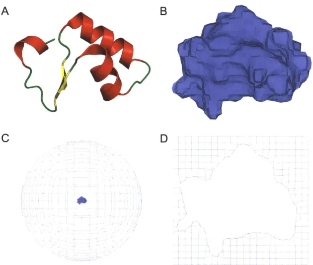
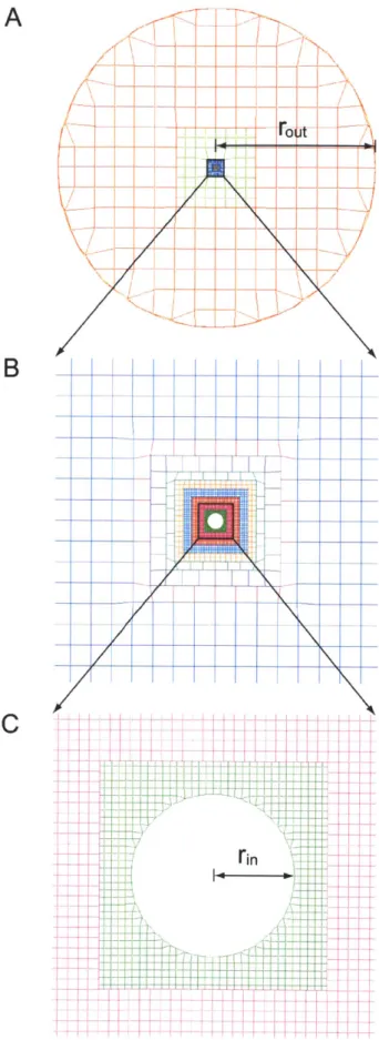
1-8 Normalized actual solution time per conformation for the subspace iteration method versus the number of conformations analyzed in the conformational change pathway of adenylate kinase using 100 and 20 norm al m odes . . . . 40 2-1 Finite element solvent model of crambin (Protein Data Bank ID 2FD7). 52 2-2 The mesh between the inner and outer sphere surfaces (in cross-section). 60

2-3 Error in the calculated translational and rotational diffusion coeffi-cients of the inner sphere versus the fraction of the nodes on the outer sphere surface that are unrestrained, rfree. . . . . 61

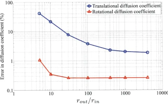
2-4 Error in the calculated translational and rotational diffusion coeffi-cients of the inner sphere versus the ratio of rout to rin. . . . . 62 2-5 Error in the calculated translational and rotational diffusion

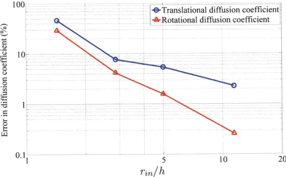
coeffi-cients of the inner sphere versus the ratio of ri, to h. . . . . 63 2-6 Root-mean-square fluctuations of -carbons of crambin obtained using

the FEM and the RTB procedure. . . . . 68 2-7 Relaxation times of the critically damped or over-damped Langevin

modes of crambin calculated for different solvent viscosities that heav-ily correlate with non-zero vacuum normal modes 1-3 of crambin. . . 72 3-1 Overall structure of H. sapiens fascin-1. . . . . 79 3-2 Structure and sequence analyses of the P-trefoil fold. . . . . 80 3-3 _{Multiple sequence alignment of homologous fascins . . . . 83}

3-4 Residues suggested to stabilize the -trefoil cores and lobes of fascin-1 84

3-5 Conservation grade and solvent-accessible surface burial of surface residues of the lobes of fascin-1 . . . . 86 3-6 _{Close-up view of highly conserved interfacial residues H139, Q141,}

S259, R383 and R389 in stick representation. . . . . 87 3-7 Residue conservation near putative actin-binding sites of fascin-1 . . . 88

3-8 Dynamically correlated domains of fascin-1 . . . . 90

A-i (A) RMSDk and (B) ARMSD k versus conformation number for the

1843-conformation pathway. . . . . 101 A-2 ARMSD versus conformation number for the (A) 1001-, (B) 101-,

and (C) 11-conformation pathways. . . . . 102 B-i Root-mean-square fluctuations of x-carbons obtained using the FEM

C-1 Analysis of structural alignments of fascin-1 domains with other

@-trefoil fold dom ains . . . 108

C-2 Conservation of residues suggested to stabilize the f-trefoil core and solvent accessible surface burial upon

B-trefoil

domain-domain associ-ation within each lobe of fascin-1 . . . 109

C-3 Distributions of pair-wise sequence identities of -trefoil domains and hom ologous fascins . . . . 110

C-4 Histograms of conservation grades across homologous fascins . . . . . 111

C-5 Functional analysis of residues of fascin-1 . . . 112

C-6 The two lowest normal modes of fascin-1 . . . 113

C-7 Correlated dynamical motions of fascin-1 . . . 114

C-8 Analysis of correlation coefficients between C, atom thermal fluctua-tions in fascin-1 . . . 115

List of Tables

2.1 Experimental values of the translational and rotational diffusion coef-ficients of 10 different proteins. . . . . 64 2.2 _{Calculated values of the translational and rotational diffusion}

coeffi-cients of 10 different proteins for the hydration layer thicknesses of 0 and 1 A . . . . 65 2.3 _{Calculated values of the optimal hydration layer thicknesses and the}

errors in the translational and rotational diffusion coefficients of 10 different proteins. . . . . 66

2.4 Highest overlap scores and corresponding critically damped or over-damped Langevin modes and relaxation times for the 10 lowest non-zero vacuum normal modes of crambin. . . . . 70 2.5 Number of critically damped or over-damped Langevin modes of

cram-bin at different solvent viscosities. . . . . 71 3.1 Average generalized linear mutual information coefficient and fraction

of residues that are in contact

(% in parentheses) for the five clusters

in fascin-1 shown in Fig. 3-8... . . . . . . . . . 91

C. 1 Solvent-accessible surface area

(A

2

)

buried between t-trefoil

domain-domain interfaces in fascin-1. . . . 116

C.2 RMSDs between the pair-wise aligned

B-trefoil

domains of fascin-1

(F1-F4) given in

A

for each pair of domains. . . . . 116 C.3 Sequence identity between domains of fascin-1 and other f-trefoil

C.4 Structural similarity between fascin-1 domains and other

B-trefoil

do-mains available in the PDB. . . . . 117 C.5 Residue type, number of residues of specific residue type, fraction of

residues of specific residue type (in parentheses) and residue num-bers of the fifty-one highly conserved residues across homologous fascin molecules that are not included in the set of hydrophobic core stabiliz-ing residues, interfacial residues, and residues 29-43 (see also Fig. C-5).118

C.6 Residue type, residue number, and conservation grades across

B-trefoil

domains (CGTD) available in the PDB, conservation grades across homologous fascin (CGHF) molecules, fraction of corresponding column which is of type "gap" (FCCTG) in the structure-based sequence align-ment of the 59 r-trefoil domains available in the PDB, and poten-tial functional reason for conservation of the fifty-one highly conserved residues across homologous fascin molecules that are not included in the set of hydrophobic core stabilizing residues, interfacial residues, and residues 29-43 (see also Fig. C-5). . . . 119

C.7 61 sequences homologous to fascin-1 retrieved from the NCBI [4] and

Introduction

Proteins are essential to organisms and play a central role in almost every biological process. Based on their functions, proteins can be divided into different classes. Structural proteins such as F-actin and microtubules are a class of proteins that are used in the cytoskeleton of cells and are responsible for the cell geometry. Another class of proteins are enzymes, which are catalysts and accelerate the chemical reactions occurring within organisms. There are also many other proteins that play roles in cell adhesion, cell cycle, cell signalling, etc.

The conformational dynamics and mechanics of proteins are of great importance to many biological functions, ranging from transcription and translation to cell di-vision and migration. Numerical methods, such as molecular dynamics (MD) and normal mode analysis (NMA), may give insight into the mechanical properties and dynamic behavior of proteins. Unlike MD, which needs to perform time-consuming time-integrations of the full set of governing equations of motion, NMA examines only harmonic oscillations of the protein around its ground-state conformation. As a result, NMA can be employed to analyze many protein motions that are currently inaccessible to MD. For example, NMA has proven successful in analyzing the func-tional motions associated with large macromolecules, such as myosin

[5,

6], kinesin

[5, 7], microtubules [8], and F-actin [9].

Over the last few decades, significant effort has been directed towards further improving the computational efficiency and accuracy of NMA for analyzing the con-formational dynamics and mechanics of proteins. For example, one of the main time-consuming parts of NMA, which has attracted much attention, is solving the eigenvalue problem associated with the protein model. However, in spite of all the

effort [10, 11], the all-atom NMA of many protein motions, such as conformational change pathways of large macromolecules, is still almost infeasible due to the lack of a computationally efficient and robust eigenvalue solver. Additionally, since the effects of solvent friction on proteins are generally ignored in NMA, the time scales of protein functional motions cannot be predicted correctly using eigensolutions. Also, it is expected that the normal modes of proteins are altered substantially when the effects of solvent-damping are incorporated into NMA [12].

The present work focuses on both developing a computationally efficient and ro-bust eigenvalue solver and incorporating the solvent-damping effects into NMA. Also, here NMA along with other computational procedures, such as sequence conservation analysis, are employed to gain insight into the functional mechanism of Homo sapiens fascin- 1, an F-actin crosslinking protein.

In Chapter 1, we first review briefly the standard subspace iteration (SSI) method, a widely used eigenvalue solver in engineering problems

[13].

Then, we present a new algorithm to optimize the number of iteration vectors employed in the method [14]. We subsequently apply the improved method to two proteins to illustrate its use in protein NMA. A particularly important observation is that with the new variant of the SSI method CPU time scales linearly with the number of eigenpairs sought [14], as in the Lanczos method [15]. Additionally, it is demonstrated that the SSI method is well-suited to the analysis of protein conformational change pathways, where hundreds of normal mode analyses may be performed in nearby conformations

[16].

In Chapter 2, we first review the Langevin mode analysis developed by Lamm and Szabo [17] to incorporate the effects of solvent-damping into the standard NMA. Then, we present a new algorithm that calculates a solvent friction matrix using the finite element method (FEM) to account for the solvent-damping effects. The algorithm proves successful in calculating the diffusion coefficients of a sphere and 10 proteins with various molecular weights, ranging from 7 kDa to 233 kDa. We subsequently couple the solvent friction matrix and the stiffness and mass matrices calculated using the FEM [18] to obtain the Langevin modes and corresponding relaxation times of

crambin, a small protein with 46 amino acids. The obtained results are then compared with those calculated using bead models

[19].

In Chapter 3, we first examine the structure of Homo sapiens fascin-1 [20], an actin-binding protein that is present predominantly in filopodia. The structure re-veals a novel arrangement of four tandem

B-trefoil

domains that form a bi-lobed structure with approximate pseudo 2-fold symmetry. We subsequently apply sequence conservation analysis to the protein to investigate its structurally and functionally im-portant regions. The results confirm the importance of the hydrophobic core residues that stabilize the f-trefoil fold, as well as the interfacial residues that are likely to stabilize the overall fascin molecule. Additionally, sequence conservation analysis in-dicates highly conserved surface patches near the putative actin-binding domains of fascin. Conformational dynamics analysis also suggests these domains to be coupled via an allosteric mechanism that might have important functional implications for F-actin crosslinking by fascin.

Chapter 1

The subspace iteration method in

protein normal mode analysis

Normal mode analysis (NMA) plays an important role in relating the conformational dynamics of proteins to their biological function [11]. In classical NMA [21, 22], pro-tein atomic degrees of freedom are treated explicitly in solving the generalized eigen-value problem in a biologically relevant conformation, typically for the lowest twenty to one hundred normal modes that represent the largest conformational fluctuations of the molecule. In the analysis of conformational transitions, numerous normal mode analyses may be performed for the same protein in nearby conformations [23].

NMA provides a considerable computational advantage over molecular dynamics

because of the elimination of time-integration and explicit solvent degrees of freedom. Nevertheless, significant effort has been directed towards further improving the com-putational efficiency of NMA to enable its application to ever-larger supramolecular complexes including viral capsids, molecular motors, and the ribosome (Ref. [16] and references therein). Particular attention has been directed to the development and application of coarse-grained protein models such as elastic network and related models [18, 24], whereas somewhat less attention has been paid to the development of algorithms that improve the computational efficiency of all-atom protein NMA itself. Such developments are of interest because they preserve the explicit representation of atomic degrees of freedom and their solvent-mediated interactions as modeled by

implicit solvent force-fields. The explicit representation of atomic interactions is im-portant to model accurately a number of biological processes, including interactions between proteins and nucleic acids [25], as well as small molecules in rational drug design [26]. Additionally, the role of allosteric regulation of binding affinity and catal-ysis by at-a-distance mutations remains an interesting and open area of research that may require all-atom modeling to understand fully [27].

The subspace iteration method was originally developed by K. J. Bathe for the solution of frequencies and mode shapes of macroscopic structures such as buildings and bridges using finite element analysis (FEA) [28, 29]. In those applications, rela-tively few frequencies and corresponding mode shapes were sought, such as the lowest 10-20 eigenpairs in models containing a total of 1000-10,000 degrees of freedom. Since its development, however, the subspace iteration method has been used extensively in the FEA of considerably larger systems reaching millions of degrees of freedom, and naturally has attracted significant attention for improvements as a result (see for example Refs. [30-37]).

The subspace iteration method is a particularly attractive approach to protein

NMA because the procedure (1) is designed specifically for the calculation of the

low-est eigenpairs of large systems; (2) uses previously calculated eigenvectors from nearby conformations to speed up significantly the solution of eigenpairs in nearby confor-mations of interest; (3) is computationally robust; and (4) is amenable to parallel-processing.

The original development of the method was based on the earlier use of the Ritz method, and relates to the works of Bauer [38] and Rutishauser [39]. Key devel-opments for its practical use in structural engineering were the specific steps in the iteration method, the construction of the starting iteration vectors, the use of an effective number of iteration vectors, the use of error measures, and the Sturm se-quence check [28]. A convergence analysis of the subspace iteration method is given in Ref. [40]. The method is also abundantly used in the solution of linearized buckling problems [13], which is applicable to calculations of the stability of the cytoskele-tal polymers filamentous actin and microtubules, as well as viral capsids and other

supramolecular assemblies with mechanically related biological function [18].

An additional leading approach to NMA in the structural mechanics community is the Lanczos method [15], advanced particularly by Paige [41] and others [42]. Initially, the Lanczos method exhibited instabilities due to loss of orthogonality of the iteration vectors employed. This shortcoming, however, has been largely overcome, and when implemented properly the method is highly efficient. A particular asset of the method is that computational effort scales about linearly (neglecting the effort for the initial factorization) with the number of eigenpairs sought, a property that is not generally satisfied by the traditional subspace iteration method. An important property of both the subspace iteration and Lanczos procedures is that they solve directly for the eigenpairs sought instead of calculating intermediate matrices first, as if all eigenvalues were desired. This property contrasts with the approach of the Householder-QR method [13], for example, which becomes prohibitively expensive computationally and in memory as the size of coefficient matrices increases. At present, the Lanczos and subspace iteration methods are the two most widely used techniques for the solution of large eigenvalue problems in FEA, when coefficient matrices are of order

10,000-10,000,000. For these reasons, any significant improvements to these methods

are of great interest.

Recently, considerable effort has been directed towards using parallel processing in FEA, in shared-memory and distributed-memory processing modes. Whereas the Lanczos method can intrinsically (largely) be parallelized only in the factorization of the stiffness matrix and the forward reduction and back-substitution of the individual vectors, the subspace iteration method allows in addition the parallel solution of

multiple iteration vectors which can result in a large computational benefit. However,

there is also interest in improving the method in other ways, and in particular, for the solution of eigenproblems in which relatively many eigenpairs need to be calculated.

As mentioned earlier, a key step in the subspace iteration method is the establish-ment of effective starting iteration vectors, which implies using an optimal number of iteration vectors. The objective of the present work is to apply the subspace iter-ation method to the normal mode analysis of proteins, and to introduce a significant

improvement upon the original implementation regarding the choice of the number of iteration vectors. In the following sections, we first review briefly the standard sub-space iteration method and discuss its inherent value for the solution of frequencies and mode shapes of proteins. We, subsequently, present a new algorithm to estab-lish an effective number of iteration vectors, illustrating the use of this algorithm in some applications. A particularly important observation is that computational ef-fort increases linearly with the number of eigenpairs sought in the solutions obtained with the improved subspace iteration method, as in the Lanczos method. To focus on our new development only, and to compare results obtained with the traditional and improved methods, we employ a basic implementation without parallelization of the code, running in-core on a single processor workstation. Moreover, we provide only relative solution times, which are largely independent of the machine used. Al-though these times thereby represent practically "machine-independent" algorithmic improvements, actual solution times will naturally depend on the specific machine employed and will decrease as computational hardware becomes more efficient.

1.1

Methods

1.1.1

The basic subspace iteration method

We consider the generalized eigenvalue problem,

Kp

AMp

(1.1)

where K and M are symmetric matrices of order n, K is positive definite, and M is positive semidefinite. We seek the smallest p eigenvalues A,, A2, ..., A, and corre-sponding eigenvectors pi, <p2, ..., p with the ordering,

A < A ... < A_ _(1.2)

Kqp = AiMpi; i= 1, ... , p (1.3)

and

(1.4)

(pi TKwpy = Aiotj

where 63 is the Kronecker delta. The basic equations used in the subspace iteration method are as follows [13]:

Step 1: Establish q starting iteration vectors in X1

Step 2: Iterate with k= 1, 2, 3, ..., until convergence

KXk+1 = MXk (1.5) - T Kk+1 = Xk+1 KXk+1 Mk+1 = k+1 MXk+1 Kk+lQk+l = Mk+lQk+1Ak+1 (1-7) Xk+1 = Xk+lQk+l (1.8)

Step 3: Perform the Sturm sequence check.

Hence, the procedure consists of three distinct solution steps. First, the q starting iteration vectors in X1 are established, q > p, where X1 is a matrix of dimension

n x q. Second, iteration is performed using Eqs. 1.5-1.8, for k = 1, 2, ... until the

convergence tolerance below is satisfied, where Qk+1 and Ak+1 store the eigenvectors

and eigenvalues corresponding to the subspace matrices Kk+1 and Mk+1. Finally, the

Sturm sequence check is performed.

Let Ai(k) be the approximation for A2 calculated in the (k - I)th iteration, we have

convergence to an accuracy of 2 x s digits in the eigenvalues when for i = 1, ..., p

[1 (-k)) (k)T 2 - 1/2 < w2s 1)

(qj k)) (k)

where q(k) is the vector in the matrix Qk corresponding to Ai(k). The eigenvectors will only be accurate to s digits and the theoretical convergence rate of the vectors is Ai/Aq+1. Thus, there is a higher convergence rate for a smaller eigenvalue and its corresponding eigenvector. Although these convergence rates correspond to the theoretical values [13, 40], they are usually also observed in actual computations. The Sturm sequence check is carried out to ensure that the lowest p eigenpairs, that is,

(Ai, pi), i 1, ..., p, have indeed been calculated [13, 28]. If the Sturm sequence check

is not passed, the iteration is continued with a larger number of iteration vectors. Considering Eqs. 1.5-1.8, it is seen that the method can be programmed efficiently for parallel computations. The factorization of the coefficient matrix and the forward reductions and back-substitutions of each individual vector can be parallelized. In

addition, the solution of the q vectors can be distributed to different processors and also the computation of the subspace matrices Kk+1 and Mk+1 can be parallelized.

An important difference between the coefficient matrices of structural FE as-semblages and of proteins is that the latter have much larger bandwidths because of long-range nonbonded electrostatic, and to a lesser extent van der Waals, interactions that introduce broad coupling between protein atoms. Thus, for a given number of degrees of freedom, the factorization of the matrix and solution of the vectors in

Eq. 1.5 constitute a much larger computational effort than in standard FE solutions.

Although parallel processing can be very important for this reason, we do not address this computational issue further in the present work.

Using the earlier equations, it is critical to establish effective starting iteration vectors for two reasons. First, if the subspace of these vectors contains the exact eigenvectors, theory states that a single iteration will result in the exact eigenvalues and vectors sought. Here, we simply use the algorithm of Ref. [28] (also given in Ref. [13]), to construct the starting iteration vectors. In cases where better starting

vectors are known from an existing solution, such as in conformational change path-way analyses of proteins where eigensolutions may be performed numerous times for small changes in protein conformation

[23],

the algorithm of Ref. [13] is used only for the first eigensolution. Thereafter, the previous solution from the nearest-neighbor conformation provides the starting iteration vectors for the next eigensolution. Sec-ond, an effective value of q needs to be used because the convergence rate to an eigenvector is given by Ai/Aq+1. If q (> p) is small, a relatively large number of

itera-tions are required to converge. In contrast, if q is large, fewer iteraitera-tions are required for convergence, but each iteration is computationally more costly. Thus, use of an optimal value of q is highly desirable. Calculation of an effective value of q for the frequency and mode shape solutions of proteins is addressed in the next section.

1.1.2

The algorithm to calculate the number of starting

it-eration vectors

An important observation regarding proteins is that the magnitudes of their eigen-values increase nearly linearly with increasing wave-number [43, 44], as shown for T4-lysozyme in Fig. 1-1. This characteristic of proteins may be used to find an effec-tive value of q for the subspace iteration method.

Assume that we order the iteration vectors in Xk naturally so that they correspond to increasing eigenvalues, with the first vector corresponding to A1 . Then the last

iteration vector to converge is the pth vector in Xk and its rate of convergence is A .

Additionally, after the ith iteration, the norm of the vector difference between the pth

M-orthonormalized eigenvector and its current approximation (the error vector c) is given by,

e (current)|

= jJ

)

(initial) (1.10)

where e (initial) is the initial error vector. To reach s-digits of accuracy in the

0.04 0.035 04 0.03-0.025 0.02 3 0.015 0.01 0.005 0 20 40 60 80 100 Eigenvalue number

Figure 1-1 - The lowest one hundred eigenvalues (Ai) of T4-lysozyme (Protein Data Bank ID 3LZM) [1]. (The first six zero eigenvalues correspond to rigid body modes.)

AP e (initial) 10-s (1. 11)

Aq+1

and, therefore, require 1 iterations for the vector to converge, where 1 is given by,

In (10-/ e (initial)) _(1.12)

In (A,/Alq+1)

Next, we use the fact that the eigenvalue magnitudes increase linearly and assume that for different values of q, the norm of the initial error vector for the pth iteration vector is the same. Additionally, the first six eigenvalues are zero. This implies that the K matrix is singular. To use the subspace iteration method, we perform a shift

p on the K matrix to have a positive definite matrix, see Ref. [13]. We use p to be a

very small value, p = -1 x 10-6. Therefore, ' is approximately equal to - .

Aq+1 (q-5-p)

Since p is very small, it can be neglected and ) _Eq. is approximated as ( -6. Then_{v i(q.e i}

In (10-S/ 1| c(initial)1) (1.13)

In ((p - 6) / (q - 5))

However, an operation count tells that the following number of numerical opera-tions are needed for 1 iteraopera-tions with q vectors

[13],

in (10-s/ & (initial)||)

TCC =

(2nq +

2nq2 + 3ng) (1.14)

In ((p - 6) / (q - 5))

where TCC is the Total Cost of Computation for 1 iterations, n is the order of the K and M matrices, and m is the half-bandwidth (assumed to be full) of the K matrix. As the column heights of K vary, an average or effective value for m must be used

[13]. Although we refer to TCC in Eq. 1.14, in reality we only have the total number

of arithmetical operations. As our only purpose is to find an effective value of q for each p, and we also know that,

C = In

(10-'/||E (initial)

where c is an unknown constant, we may use,

TCC = c (2nmq + 2nq2 _{+ 3nq) (1.15)}

ln ((p - 6) / (q - 5))

Minimizing this expression with respect to q we find an approximation for the best q to obtain the p eigenvalues and vectors in the least amount of computational time. Because a closed-form solution does not exist, we solve for q by iteration. Note that this analysis does not provide the actual computational effort required (since the constant c is unknown) but only that the minimum is obtained when using the value of q given by minimizing TCC in Eq. 1.15.

Fig. 1-2 shows the normalized actual solution time and TCC to calculate the lowest 100 eigenvalues with six digits of accuracy for T4-lysozyme using different numbers of iteration vectors. The iteration times are normalized by the maximum actual iteration time and, since the constant c in Eq. 1.15 is unknown, TCC is scaled such that the iteration times are equal at the minimum of TCC.

0.6

Z0 0.

0.2

00 150 200 250 300 350 400

Number of iteration vectors

Figure 1-2 - Normalized actual iteration time and normalized TCC to calculate the first

one hundred eigenvalues for T4-lysozyme (Protein Data Bank ID 3LZM) [1].

As seen in Fig. 1-2, prediction of the relative computational cost of calculating the lowest eigenvalues with different numbers of iteration vectors by Eq. 1.15 is acceptable. Next we illustrate the use of the value of q in the normal mode analyses of two proteins.

1.2

Results

1.2.1

Illustrative solutions

In this section we use the subspace iteration method for the calculation of the frequen-cies and normal modes of two proteins. In each case we use the standard subspace iteration method as published in Refs. [13, 28] including the algorithm to construct

all starting iteration vectors. We use the standard value q= min

{2p,

p+8}, referred

to as the traditional subspace iteration method, and this method with the value of

q that minimizes TCC in Eq. 1.15, referred to as the improved subspace iteration

method. We intentionally do not use any other acceleration techniques, such as given for example in Ref. [30], to identify clearly the improvements achieved solely by use

of the value of q derived earlier.

In each solution we employ the skyline solver of Ref. [13] for Eq. 1.5. Although we recognize that a sparse solver could lead to significantly improved solution times

[45],

we do not expect our fundamental observations regarding the performance of

the method to be affected. We note that the solution times given always include all operations of the subspace iterations. Additionally, in an effort to present machine-independent conclusions regarding performance of the algorithms, we present normal-ized solution times instead of actual solution times, where normalnormal-ized time is equal to actual time divided by the maximum solution time measured in each case.

G-actin

The initial structure of ADP-bound G-actin is taken from the work of Otterbein et al. [2] (Protein Data Bank ID 1J6Z; residue numbers 4-372). The stiffness matrix of order

10,608 for this protein was computed in CHARMM version 34b1 [46] using the implicit

solvation model EEF1 [47]. Steepest descent minimization followed by adopted-basis Newton-Raphson minimization is performed in the presence of successively reduced harmonic constraints on backbone atoms to achieve a final root-mean-square (RMS) energy gradient of 2 x 10-4 kcal with corresponding RMS deviation between the

X-(Mo X A)

ray and energy-minimized structures of 1.4

A

(Fig. 1-3). Computations are performed on an Intel Xeon 5120 with 1.86 GHz and 4 GB RAM in single processor mode.

Considering the eigenvalue problem, different numbers of the lowest eigenvalues with six digits of accuracy of this protein have been obtained using the traditional and improved subspace iteration methods. Fig. 1-4 provides normalized solution times versus the required number of lowest eigenvalues for G-actin, and also provides in parentheses the number of iteration vectors q used in the improved subspace iteration method in each case. It is evident that a significant improvement in the subspace iteration method is achieved by use of the calculated values of q.

As already noted, normalized solution times in Fig. 1-4 are defined as the actual solution times divided by the maximum solution time encountered in the analysis. The maximum solution time (13,939 seconds clock-time) in this case is the time

Figure 1-3 - _{G-actin-ADP. Schematic representation of the energy-minimized molecular}

structure analyzed with subdomains colored according to the definition of Kabsch et al. [48], Subdomain 1 is colored blue, subdomain 2 is colored red, subdomain 3 is colored green, and subdomain 4 is colored yellow. ADP is shown in van der Waals representation. Figure rendered using PyMOL [49].

subspace iteration 0.7 0.6 -0.5

zo0.4- 0.1- 0--10 50 100 150 200 250 300 (20) (124) (244) (358) (467) (573) (676)

Required number of the lowest eigenvalues (Optimal values of q )

Figure 1-4 - Normalized solution times versus required number of the lowest eigenvalues with six digits of accuracy for G-actin (Protein Data Bank ID 1J6Z) [2] using the traditional and improved subspace iteration methods; the value of q used in each case with the improved subspace iteration method is given in parentheses.

required to compute the lowest 300 eigenpairs with the traditional subspace iteration method. This solution time is quite large for the reasons mentioned earlier.

Pertussis toxin

The next protein examined is pertussis toxin (chains A-F). Initial coordinates are taken from the work of Stein et al. [3] (Protein Data Bank ID 1PRT). Like for G-actin, CHARMM version 34b1 [46] with the implicit solvation model EEF1 [47] is used to obtain the energy-minimized structure (Fig. 1-5) and calculate the Hessian, which has dimension of order 26,664. Steepest descent minimization followed by adopted-basis Newton-Raphson minimization is performed in the presence of successively reduced harmonic constraints on backbone atoms to achieve a final root-mean-square (RMS) energy gradient of 3 x 10-4 kcal with corresponding RMS deviation between the

(moixA)

X-ray and energy-minimized structures of 1.6

A.

Computations are also performed on an Intel Xeon 5120 with 1.86 GHz and 4 GB RAM in single processor mode.

Fig. 1-6 shows the measured normalized solution times versus the required number of the lowest eigenvalues for this molecule, and also gives in parentheses the number of iteration vectors q used in the improved subspace iteration method in each case. Again, significant computational savings are achieved when the improved iteration method is used.

1.2.2

Conformational change pathway analysis of adenylate

kinase

To illustrate the benefit of employing the subspace iteration procedure to analyze conformational change pathways of proteins, we apply the procedure to the open-to-closed transition of adenylate kinase (PDBIDs 4AKE [50] and 1AKE [51] for the open and closed conformers, respectively)(Figs. 1-7-A and 1-7-B). In the absence of molecular dynamics or other all-atom trajectory, we employ the elastic-based FE model applied previously to protein NMA to generate the conformational change pathway [18]. The initial model is defined by the open conformation of the protein.

Figure 1-5 - Pertussis toxin. Schematic representation of the energy-minimized molecular

structure analyzed with subdomains colored according to the definition of Stein et al. [3],

S1 is colored green, S2 is cyan, S3 is purple, S4 is red, and S5 is yellow. Figure rendered

using PyMOL [49].

subspace iteration 0.6 0.1 ---0 A 0Z- 0.4 0.3 0.2k 0.1L 0 10 50 100 150 200 250 300 (20) (126) (253) (374) (492) (607) (718)

Required number of the lowest eigenvalues (Optimal values of q)

Figure 1-6 - Normalized solution times versus required number of the lowest eigenvalues

with six digits of accuracy for one of two molecules from pertussis toxin (Protein Data Bank

ID 1PRT; Chains A-F) [3] using the traditional and improved subspace iteration methods;

the value of q used in each case with the improved subspace iteration method is given in parentheses.

Following Ref. [18] the molecular volume is defined by the solvent excluded surface

(SES) using MSMS ver. 2.6.1 [52]. This SES is then decimated to a coarsened

surface using the surface simplification algorithm QSLIM [53-55], as implemented in MeshLab [56]. Finally, the decimated SES is imported into the finite element analysis program ADINA ver. 8.5 (Watertown, MA), where the molecular volume is meshed automatically using 3D four-node tetrahedral elements [18]. The protein is assumed to behave as a linear, isotropic material with homogeneous mass density of 1420 S,

elastic Young's modulus of 4.9 GPa, and Poisson's ratio of 0.3. The mass density is obtained from the molecular weight and molecular volume of the open conformation. The Young's modulus is obtained by fitting thermal fluctuations of a-carbon atoms in the finite element model to those obtained using the Rotation Translation Block procedure [57, 58] at room temperature in CHARMM, where one block per residue and the implicit solvation model EEF1 [47] are employed (see Appendix B).

The conformational change pathway of adenylate kinase is generated according to

the procedure of Tama, Miyashita, and Brooks [59]. Starting from the initial, open conformation, K and M matrices are generated for the FE model using ADINA. The traditional subspace iteration procedure is then used to calculate the first 100 eigen-pairs of the model with four digits of accuracy for the eigenvalues. The FE model interpolation functions are used to interpolate the eigenvectors, pi k, corresponding

to the FE nodal positions to their values, Cik, at the positions of the a-carbons, where i and k denote the number of the eigenvector and conformation, respectively. To generate the next conformation, the difference vector between the positions of the a-carbons in the kth conformation and those of the closed conformation, Ark, is

projected onto the eigenvectors corresponding to the a-carbons, cik -

#k

Ark . C,

where

#k

is a parameter between zero and one [23, 59] (see Appendix A). cik is the contribution of the ith eigenvector to the displacement of the L-carbons in the kth step. Positions of all non-a-carbon atoms are updated using the FE displacement interpolation functions in the current conformation. This procedure is repeated until the root-means-quare-difference (RMSD) between the current positions of c-carbons and those of the closed conformer is less than or equal to 1

A.

In this approach to

B

Figure 1-7 - Conformational change pathway of adenylate kinase. (A) Schematic repre-sentation of the open conformation of adenylate kinase (Protein Data Bank ID 4AKE [50]). (B) Schematic representation of the closed conformer of adenylate kinase (Protein Data Bank ID lAKE [51]). (C) Schematic representation of the open-to-closed transition. The root-mean-square-difference between the positions of c-carbons in the closed conformer and that of the red, yellow, green, violet, and blue conformations is 7.14, 5.25, 3.5, 1.75, and 0

generating the conformational change pathway, the eigenvectors of the current con-formation are used as the starting vectors for the eigenvalue problem of the next conformation, excluding the first step, which is also excluded from the solution time per conformation presented below because it constitutes a small and invariant com-ponent of the total solution time in each case. An initial conformational change pathway of 1843 conformations is generated, from which subsets of 1001, 101, 11, and 1 conformation are chosen with nearly constant differences in RMSD between x-carbon positions of each successive conformation and the closed conformation (see Appendix A) (Fig. 1-7-C). Computations are performed on an Intel Xeon E5405 with 2.00 GHz and 16 GB RAM in single processor mode.

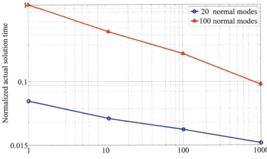
The solution time per conformation for the subspace iteration procedure decreases monotonically with increasing number of conformations employed in the conforma-tional change pathway (Fig. 1-8). Normalized time is equal to the actual solution time divided by the maximum solution time measured in the 100 normal mode case. As an increasing number of conformations is employed, normal mode solutions from neighboring conformations become increasingly better choices for the starting normal modes of neighboring conformations, resulting in the observed decrease in solution time per conformation. This result is true whether 20 or 100 eigenvectors are solved for (Fig. 1-8), and is additionally expected to be independent of the number of degrees of freedom in the model. Although it is of interest to understand the detailed solution-time properties of the subspace iteration procedure in conformational change pathway analysis (e.g., dependence of solution time per conformation scaling with model size, number of normal modes computed, etc.), such analysis is reserved for future work.

1.3

Important properties of the subspace iteration

method

In evaluating the effectiveness of any numerical procedure, it is clearly valuable to make a thorough comparison with existing methods [10, 15, 21]. In the present

-- 20 normal modes! - 100 normal modes]

0

1 10 100 1000

Number of conformations

Figure 1-8 - Normalized actual solution time per conformation for the subspace iteration method versus the number of conformations analyzed in the conformational change pathway of adenylate kinase using 100 and 20 normal modes.

case, such comparison is unfortunately complicated by a number of factors, including the requirement that each method employs the same convergence tolerance and is implemented in the optimal manner. Even then, results would depend on whether the computation is performed in- or out-of-core, the type of parallel processing used, the degree of energy-minimization performed in the use of some methods, and so on. While such a comparison would clearly be of value, it is outside the scope of the present work. Nevertheless, we would like to point out several important properties of the subspace iteration procedure, and in particular contrast these properties with corresponding properties of the Lanczos method.

The subspace iteration procedure converges monotonically and robustly to the number of frequencies and mode shapes sought. In each subspace iteration, inverse iteration is performed on a q-dimensional subspace and a Rayleigh-Ritz analysis ex-tracts the best approximations to the p normal modes sought. Best here refers to minimization of the Rayleigh quotient on the subspace [13, 40]. As the q-dimensional subspace is rotated towards the least dominant p-dimensional subspace within each

iteration, the NM approximations become more accurate. If only low accuracy in the normal modes is needed, only a few subspace iterations may be required.

Solution time in the Lanczos method scales approximately linearly with the num-ber of eigenpairs computed. The traditional subspace iteration does not typically display this scaling when many frequencies and mode shapes are calculated (e.g.,

> 20) and a single processor is employed. In the present work, however, we observed that the subspace iteration method with the improved selection of the number of iter-ation vectors also resulted in linear scaling of solution time with the number of normal modes sought. As expected, we additionally observed a significant decrease in compu-tational time when the NMA was performed on multiple neighboring conformations, because the method uses normal mode solutions from neighboring conformations to accelerate subsequent solutions. This is an important property of the subspace iter-ation procedure that is not a property of methods that start with individual vectors, such as the Lanczos algorithm. Additional acceleration might be achieved for NMA of single conformations by exciting principally the dihedral angles to choose starting vec-tors that span a subspace that is closer to the required least dominant subspace than the algorithm employed here [13, 28]. In addition, acceleration techniques published previously could be implemented [30, 35].

A final important computational property of any NMA procedure is the

possi-bility to use parallel processing (with shared and distributed memory), such as im-plemented for the Lanczos procedure in the publically available program ARPACK

[60]. Although the calculations in the subspace iterations (Eqs. 1.5-1.8) lend

them-selves naturally to parallel processing, the actual benefits achievable in comparison to the Lanczos procedure, which operates sequentially on individual vectors, remain to be established. Use of a combination of the basic steps in the subspace iteration and Lanczos methods, using the best ingredients of each technique and taking into account parallel processing, would be of interest to reach a more effective method. Further investigation is required to identify the appropriate next steps to take in this research direction.

1.4

Concluding remarks

The objective of this chapter was to present the application of the subspace itera-tion method to the normal mode analysis of proteins and to provide an algorithm for the calculation of an effective number of iteration vectors. We demonstrated use of an algorithm to calculate the number of iteration vectors q to find p eigenpairs that improves the effectiveness of the subspace iteration method significantly for pro-teins. The algorithm results in computation time scaling linearly with the number of eigenpairs sought, as demonstrated for G-actin and pertussis toxin. The subspace iteration method is well suited to protein NMA because relatively small subsets of the total available normal modes are typically sought and numerous analyses may be performed for relatively similar conformations in conformational change pathway analyses

[23].

In such cases, the previously calculated eigensolution provides an ex-cellent set of initial iteration vectors for the subsequent solution, as demonstrated here for the open-to-closed confornational change of adenylate kinase. The subspace iteration method is additionally attractive because it is robust, in that it converges monotonically to the desired eigenvalue solution for any positive semidefinite stiffness matrix. This is of significant utility in all-atom protein NMA for two reasons. First, energy minimization to tight tolerance in the energy gradient is time-consuming and often challenging due to the rugged energy landscape of proteins, and second, energy minimization often distorts the protein structure such that it deviates significantly from the experimental crystal structure. For these reasons, and due to its relative com-putational efficiency, the robust Rotational Translational Blocks procedure [57, 58]

has gained significant popularity. However, this procedure assumes single or larger blocks of residues to be rigid, in contrast with the present implementation that re-tains all atomic degrees of freedom. Although the significant reduction in number of degrees of freedom in the former approach renders its computational efficiency high, an interesting area of future research concerns the integration of computationally ro-bust NMA methods with efficient reduced degree-of-freedom approaches that retain internal residue flexibility, as initially proposed in Ref. [57]. Incorporation of such

procedures into the finite element method would enable simultaneously calculations of protein mechanical response, as well as NMs.

Chapter 2

Finite element framework for

Langevin modes of proteins

Protein motions such as conformational changes, folding/unfolding, and ligand asso-ciation/dissociation generally occur in a physiological solvent, a viscous environment within cells. Hence, to analyze the true dynamic behavior of a protein, both the pro-tein and the solvent have to be modeled simultaneously, as in all-atom, explicit-solvent molecular dynamics [61]. However, in practice, especially for the above-mentioned long-time and large length-scale motions, the time-integration of the full set of gov-erning equations of motion performed in the molecular dynamics is infeasible. Hence, coarse-grained models have been developed to speed up the analysis of the dynamic behavior of proteins. These models can describe many protein motions which are cur-rently inaccessible to the standard molecular dynamics. For example, protein folding and unfolding have been investigated, respectively, using lattice models [62-64] and steered molecular dynamics [65]. Also, the elastic network model (ENM), a coarse-grained normal mode analysis (NMA), has been used to analyze the conformational change pathways of proteins [7, 66-68]. Generally, the effects of solvent friction on proteins are ignored in these normal mode analyses. Consequently, the frequencies of proteins calculated from the set of the governing equations of motion in a vacuum cannot be used to predict the actual time-scales of functional protein motions in a sol-vent. Also, the normal modes of proteins are altered significantly when incorporating