Effect of Non-linear Loading Paths on Sheet Metal Fracture: Large
Strain In-plane Compression Followed by Uniaxial Tension
by
Stephane Marcadet
Ingenieur de l'Ecole Polytechnique (2010)
Submitted to the Department of Mechanical Engineering
in Partial Fulfillment of the Requirements for the Degree of
Master of Science in Mechanical Engineering
at the
Massachusetts Institute of Technology
February 2012
ARCHNES
MASSACHUSETTS INSTITUTE OF TECHI'lC_(VVr
EB 1 6 1
L_-
-_-J
L BRRE
© 2012 Massachusetts Institute of Technology. All rights reserved.
Signature of Author:
---15epartment of Mechanical Engineering
January 27, 2012
Certified by:
Tomasz Wierzbicki
Professor of Applied Mechanics
Thesigupervisor
Accepted by:
David E. Hardt
Professor of Mechanical Engineering
Chairman, Committee for Graduate Students
Effect of Non-linear Loading Paths on Sheet Metal Fracture: Large
Strain In-plane Compression Followed by Uniaxial Tension
Stephane Marcadet
Submitted to the Department of Mechanical Engineering
on January 27, 2012, in partial fulfillment of the requirements for the degree of
Master of Science in Mechanical Engineering
Abstract
Advanced high strength steel sheets are rapidly entering the transport industry, as their high strength to weight ratio helps improving fuel and costs efficiency. The early ductile fracture of these materials limits their formability and crashworthiness. A phenomenological criterion to predict ductile fracture has been developed based on a law of damage accumulation weighted by the stress state. The calibration of such a model requires accurate measurements of the history of stress and strain state up to the onset of fracture. The phenomenon of localized necking occurs prior to ductile fracture in most types of loading of sheet metal. In order to measure the local state of stress and strain, a hybrid experimental and numerical method is tested. The Finite Element model can accurately predict the load displacement relation using a quadratic Hill 48 yield surface and an associated flow rule. The evolution of the local stresses and strains in the material are found to be non linear after necking. Results of such a method to calibrate the fracture criterion provide a validation of the model in a large range of loadings, including uniaxial, biaxial and shear.
The effect of a reverse loading is then explored by developing an innovative experimental procedure to adapt the hybrid method for in plane compression followed by uniaxial tension of sheet metal. An Anti Buckling Device (ABD) and special grips are developed to delay buckling of the sheet. The hybrid method requires an accurate constitutive model of the material in the case of reverse loading for the Finite Element model. A modified Yoshida hardening called IH +
LK + LNK combining isotropic hardening, linear and non linear kinematic hardening provides good prediction of the load displacement relation. An analysis of the history of local stresses and strains up to the onset of fracture suggests that limited damage is accumulated during the compression phase, validating the phenomenological model.
Thesis Supervisor: Tomasz Wierzbicki Title: Professor of Applied Mechanics
Table of Contents
I. Introduction ... 13
1.1 Background... 13
1.1.1 Ductile Fracture ... 13
1.1.2 Cyclic plasticity m odels... 14
1.1.3 In-plane compression experim ents for sheet m aterials... 15
1. 1.4 Reverse loading fracture experim ents... 16
1.2 Objectives of this thesis... 16
1.3 M aterial... 18
II Plasticity & Fracture M odels... 19
2.1 Plasticity m odel for linear loading paths ... 19
2.1.1 Plasticity M odel... 19
2.1.2 Plasticity calibration... 21
2.2 Constitutive m odeling for reverse loading ... 27
2.2.1 Kinem atics of finite strain... 28
2.2.2 Yield surface ... 28
2.2.3Associated flow rule ... 29
2.2.5 Non Linear Kinem atic hardening... 30
2.2.6 Isotropic hardening ... 31
2.2.7 Plasticity m odel param eter identification ... 31
2.3 Identification of the load path to fracture ... 33
2.3.1 Stress and Strain invariants... 33
2.3.2 M odified M ohr Coulom b M odel for fracture ... 35
Chapter 3... 37
III Fracture experim ents... 37
3.1 Experim ents ... 37
3.1.1 Specim ens... 37
3.1.2 Digital Im age Correlation... 39
3.2 Computational M odel... 40
3.2.1 Finite Elem ent M odel ... 40
3.2.2 Fracture Locus ... 42
3.3 Results... 45
3.3.1 Plasticity Validation... 45
3.3.2 Results... 48
3.3.4 Validation of the m odel ... 50
3.4 Conclusion ... 54
IV Effect of reverse loading on Fracture ... 55
Experim ental procedure ... 55
Testing M achine... 55
4.1.2 Anti Buckling Device ... 56
4.1.3 Specim en... 57
4.1.4 Digital Im age Correlation ... 57
4.1.5 Procedure ... 58
4.1.6 Experim ental results... 58
Finite Elem ent M odel ... 60
4.3 Results... 61
4.3.1 Plasticity Validation... 61
4.3.2 Evolution of Stress and Strain States ... 63
4.3.3 Dam age accumulation... 65
4.3.4 M odified M ohr Coulomb Criterion ... 67
4.4 Conclusion ... 68
References...70 Annex...74
Effect of non linear loading paths on sheet metal forming limits: large in-plane pre strain followed by uniaxial tension... 74
List of figures
Figure 1 Tensile strength versus total elongation plot of advanced high strength steels... 13
Figure 2 Uniaxial Tension test of DP780 from USS in 0 direction... 18
Figure 3 D ogbone specim ens... 21
Figure 4 Uniaxial Tension tests of Dual Phase Steel in three directions to rolling direction... 21
Figure 5 Diagram of evolution of width and transverse strain for Lankford coefficients d eterm in ation ... 2 3 Figure 6 According to Mohr at al. (2010), the Lankford r coefficient can be plotted as a function of the a orientation from 0 to 90 degrees, knowing only the three coefficients in the 0, 45 and 90 degrees directions. An obvious anisotropy can be observed. ... 24
Figure 7 Interpolation, extrapolation, and discretization of the stress strain curve. ... 25
Figure 8 Comparison of Load Displacement prediction with Isotropic Hardening in the case of linear and reverse loading ... 27
Figure 9 Interpretation of the Lode Angle in terms of principal stresses. ... 35
Figure 10 Set of specimens used to calibrate the Modified Mohr Coulomb Criterion... 38
Figure 11 Displacement measured by Digital Image Correlation using extensometer and the corresponding Finite Elem ent M odel... 39
Figure 12 On the left: last picture before the onset of fracture. On the right: first picture after fractu re ... 4 0
Figure 13 Finite Element meshes of the different specimens, and illustration of the symmetries. ... 4 1
Figure 14 Guess on the position of the element corresponding to the location of the onset of
fracture for each specim en m esh... 42
Figure 15 On the left, force versus displacement curve and displacement at fracture. On the right, strain as a function of the displacement and strain at fracture determined by the measured displacem ent at fracture. ... 43
Figure 16 Strain as a function of the thickness in the case of the punch test and strain at fracture determined by the measured thickness at fracture. ... 44
Figure 17 Comparison of experimental and computer predicted Force displacement curves and fracture locu s... 4 7 Figure 18 Strain and stress state history during loading for each test. ... 48
Figure 19 Fracture locus in terms of strain as a function of the triaxiality with the hypothesis of plane strain, and fracture locus of the experiments... 50
Figure 20 A plot of the full modified Mohr Coulomb criterion. Strain at fracture is a function of L ode angle and triaxiality. ... 50
Figure 21 Overview of the prediction of the fracture locus is terms of damage, displacement and strain thanks to the calibrated Modified Mohr Coulomb criterion. ... 53
Figure 22 Testing M achine set up... 55
Figure 23 Procedure to install the Anti Buckling Device ... 56
Figure 24 Compression Tension Specimen Geometry ... 57
Figure 25 Digital Image Correlation with extensometer through the window of the anti buckling d ev ice ... 5 8 Figure 26 Load Displacement obtained for reverse compression tension uniaxial tests ... 59
Figure 27 Mesh of the compression tension specimen ... 60
Figure 28 Overview of the computer prediction of the load displacement for each compression tension test with the optimized modified Yoshida plasticity Model... 61
Figure 29 Prediction of the load displacement for each test ... 62
Figure 30 Color coded plot of the equivalent strain in the Dogbone specimen at fracture ... 64
Figure 31 History of the loading path in the space of triaxiality and equivalent plastic strain for all levels of pre strain ... :... 64
Figure 32 History of the loading path in the space of Lode angle parameter and equivalent plastic strain for all levels of pre strain ... 64
Figure 33 History of loading path and fracture in the space of triaxiality and equivalent plastic strain considering the return to zero displacement as a new initial state ... 65
Figure 34 Dependance of the weight function of the damage accumulation model on the triax iality ... 6 6
Figure 35 Overview of the prediction of fracture of the Modified Mohr Coulomb Criterion in the case of reversed L oading ... 67
List of Tables
Table 1 Lankford Coefficients for DP780 ... 18
Table 2 Lankford C oefficients ... 24
Table 3 Yield Surface anisotropy in Abaqus ... 26
Table 4 Y ield surface anisotropy. ... 26
Table 5 Numerical values for the optimized parameters of the modified Yoshida plasticity model ... 61
Chapter 1.
I. Introduction
1.1 Background
1.1.1 Ductile Fracture
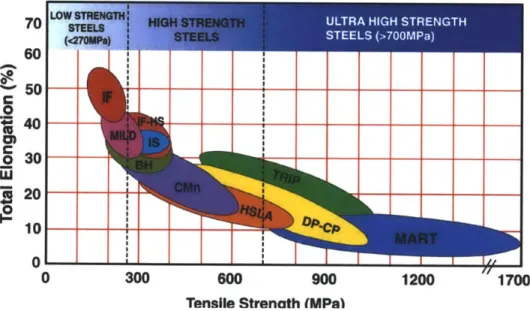
The transportation industry is putting considerable recourses to integrate high strength to weight ratio materials in the vehicles structures in order to improve fuel and costs efficiency. Advanced high strength steel sheets play a major role as they provide very high strengths at reasonable weight. The use of these materials is restricted by low ductile fracture that limits their formability and crashworthiness (Fig. 1).
70 60 50 CO o 30 j 20 10-0 0 300 600 900 1200 1700
Tensile Strenath (MPal
Figure ITensile strength versus total elongation plot of advanced high strength steels
Ductile fracture is often studied on a microscopic scale, focusing on the propagation of cracks. McClintock (1968) and Rice and Tracey (1969) were the first to show that the stress triaxiality governs the growth of voids in the material. Gurson (1977) introduced the void
volume fraction as an internal variable in a porous plasticity model. A number of modified Gurson models have been developed since, introducing notions such as the void coalescence (Tvergaard and Needleman, 1984) and void shape effects (Pardoen and Hutchinson, 2000).
As an alternative, attempts to predict ductile fracture from a phenomenological point of view have been carried out. They are based on the assumption that the onset of fracture occurs when a certain critical value of the plastic strain is reached. An accumulation of the plastic strain weighted by a function of the stress state is introduced. This weight function has recently been proven to depend on the state of stress (Bao and Wierzbicki 2003, Wierzbicki and Xue 2005, Bai and Wierzbicki 2008). Two invariants of the stress of state, triaxiality and Lode angle are taken into account.
Hancock and McKenzie's (1976) tensile tests on axisymmetric notched specimens show that the ductility decreases with triaxiality, as predicted in Rice and Tracey's (1969) fracture model. Hancock and Brown (1983) compared tests on cylindrical and flat specimens and concluded that ductile fracture limits depend on the stress state and not the strain state. More recently, numerous innovative tests have been developed by Bao (2003), Mohr and Henn (2007) and Mohr and Oswald (2008) to explore the dependency of fracture in a wide range of stress states.
1.1.2 Cyclic plasticity models.
Kinematic hardening models are most commonly used for non-proportional monotonic loadings or cyclic loadings. Therefore they seem to be a good candidate for reverse loading. Kinematic hardening parameters are used as a back stress in the yield surface formulation.
The simplest kinematic hardening model is the linear kinematic hardening law introduced by Prager (1949). In this case, the back stress evolution is unbounded and evolves along the direction of the plastic strain increment.
But linearity is rarely observed in the stress strain response. That is why a more complex kinematic hardening model is proposed by Armstrong and Frederick (1966, 2007), introducing a second term, the recall term, which activates the so called dynamic-recovery. The recall term is collinear with the back stress and is proportional to the equivalent plastic strain rate. As a result, the evolution of the back stress is no longer linear and unbounded and converges towards a saturation value under monotonic loading. As discussed by Lemaitre and Chaboche (1994), the dynamic recovery term may be interpreted as a description of the "fading memory effect of the strain path." For example, in the case of uniaxial tension, the back stress evolution asymptotically approaches a saturation value.
As an even better approximation, several such models can be added with different recall constants to form the total back stress (Chaboche et al., 1979; Chaboche and Rousselier, 1983). The use of a non linear kinematic hardening gives good prediction in the case of a cyclic loading in the range of small strains, as it is able to describe the Bauschinger effect. As a particular case of the superposition of back stresses technique, a model coupling a linear kinematic hardening and a non linear kinematic hardening gives better results in the case of mid and high strains as it describes the permanent softening behavior during reverse deformation, especially with advanced high strength steels with almost no workhardening stagnation (Yoshida et al., 2002). .
1.1.3 In-plane compression experiments for sheet materials
In order to test reverse uniaxial loading of sheet metal, in-plane compression has to be performed experimentally. This implies some technical difficulties to avoid elastic or plastic buckling of the specimens in the range of small strains. A design has originally been developed by Dietrich and Turski (1978) to compress sheet metal. Kuwabara (1995) et al. introduced an Anti Buckling Device used with a lateral blank holder to apply a pressure reaching 1% of the elastic limit. In another attempt, Yoshida et al. tried to stack several dogbone specimens to delay buckling. The stack is maintained by adhesive and placed in an anti buckling device applying up to 10% of compressive strain. Boger et al. apply a lateral pressure to the specimens using a hydraulic system through clamping plates. Several methods to take frictional effects into account
have been developed. The geometry of the specimen plays a major role in the efficiency of these experimental procedures. A double wedge system using Teflon sheets of thickness of half a millimeter has been introduced by Cao et al., providing an elastic support to the specimen.
1.1.4 Reverse loading fracture experiments
The effects of reverse loading have not yet been fully understood and explained. McClintock (1993) explained that crack nucleation can be caused by strain concentration under cyclic loading. Seok et al. (1999) showed that the fracture resistance curves decreases with decreasing minimum-to-maximum load ratio of cyclic loading and decreasing incremental plastic displacement. Harvey (2000) performed strain controlled cycling followed by monotonic tensile loading to fracture. He found by looking at the fracture surface using scanning electron microscopy (SEM) that cyclic loading increased the total number of micro voids. The aspect ratio of micro voids seemed to be only a function of the loading and showed no dependency on pre strain. Other studies were mostly focused on the effect of preloading on fracture toughness and propagation. Some studies investigated the effect of reverse loading on ductile propagation of cracks in the case of reverse bending tests of beams. Bao and Treitler (2004) investigated the effect of reverse loading on crack formation. Notched cylindrical tensile specimens have been adapted to perform compression tension tests. They proved that the pre-compression plays a very important role in the crack formation. The dimple structure observed from fracture surface is finer and the size of voids is smaller in the case of pre-compression. Particles crack along the loading direction under pre-compression loading, while particles fail in the direction perpendicular to the loading direction under tensile loading.
1.2 Objectives of this thesis
The objective of this study is to understand the effect of complex non linear quasi-static loadings on the onset of ductile fracture of advanced high strength steel sheets. The first step is the validation, in the case of a dual-phase steel, of an innovative hybrid experimental and
numerical method developed by Dunand and Mohr (2010). This method is then adapted to evaluate the effect of reverse loading on ductile fracture of sheet metal.
The hybrid method is used to characterize the ductile fracture as a function of the stress and strain state. Several types of tests are performed to observe fracture in a wide range of stress states: tensile notched- shaped specimens and a tensile specimen with a central hole, a shear test and a punch test. Most phenomenological fracture criterions require the identification of the history of equivalent plastic strain and stress state. These quantities cannot be directly measured on the experiment. Therefore, a Finite Element analysis of these tests provides the history of triaxiality, Lode angle parameter and equivalent plastic strain. The local stress and strain state evolution is non linear because of the localization of the plastic strain that leads to the necking effect. A phenomenological criterion known as the Modified Mohr Coulomb criterion to predict the quasi static ductile fracture of Advanced High Strength Steel sheets is calibrated and validated for these tests.
In the second part, an experimental technique of a pre compression on tensile specimens of sheet metal is presented. It uses an anti buckling device and special grips. Large in plane pre-compression followed by uniaxial tension tests to fracture have been performed for various levels of pre strain. A suitable plasticity model for large in plane reverse deformations is carefully developed to predict the behavior of the material. The hybrid experimental and numerical method is used to observe the history of local state of stress and strain at the fracture locus for all tests. It is found that pre compression has an important effect on the equivalent strain at fracture, but has little effect on the stress state at fracture. It is interpreted that, in the frame of the phenomenological theory of damage accumulation, little damage is accumulated during the compression phase.
1.3 Material
The detailed calibration of the Modified Mohr Coulomb criterion has been performed on a Dual-Phase steel. Its mechanical characteristics are presented in details in the following study. Sheets have a thickness of 1.44 mm.
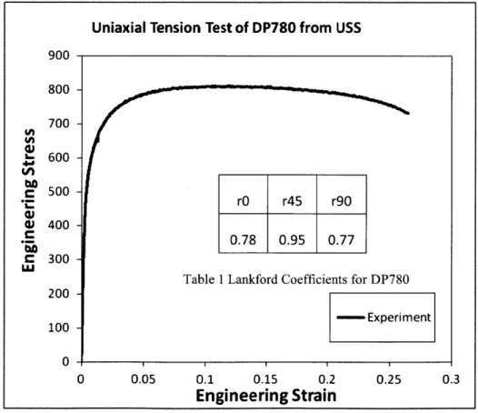
The study of the effect of reverse loading on ductile fracture has been performed on a different Dual-Phase steel, DP780, provided by US Steel (Fig. 2). Its Young modulus is 195 GPa. Its yield point is different in tension (450 MPa) and compression (510 MPa). This is due to the rolling treatment. In order to take this particularity into account, an initial value for the back stress is introduced in the plasticity model. The Lankford coefficients have been measured for this material to be able to take its anisotropy into account. Sheets have a thickness of 1.06 mm.
Figure 2 Uniaxial Tension test of DP780 from USS in 0 direction
Uniaxial Tension Test of DP780 from USS
900 -800 -700 -1 600 -c500 rO r45 r90 4) 400 -C 0.78 0.95 0.77 C 300 LU
Table 1 Lankford Coefficients for DP780 200
100 -- Experiment
01
0 0.05 0.1 0.15 0.2 0.25 0.3
Chapter 2.
II Plasticity & Fracture Models
A good understanding and modeling of the plastic behavior of the material is a necessary step towards the study of ductile fracture. Simulating the experiments in Finite Element Analysis software provides the history of the stress state and local strains during the different loading phases. The interests of this analysis are the triaxiality, load angle and local equivalent plastic strain in the elements where experimental fracture is expected to occur first. Simulation is considered as relevant if the load-displacement curves of the experiment and its computer simulation match. Therefore the measurement of these parameters is highly dependent on the plasticity model. That is why an accurate plasticity model is crucial as the damage accumulation
law is based on these parameters.
2.1 Plasticity model for linear loading paths
The Finite Element Analysis requires the determination of the plastic behavior of the material. According to Mohr at al. (2010), a standard plasticity model can be used for advanced high strength steels, featuring an anisotropic quadratic yield surface (Hill 1948), an associated
flow rule and an isotropic hardening law.
2.1.1 Plasticity Model
Hill 48 quadratic yield surface:
f(1, EP') = d - k(EP') =0 (1)
o = P(o): c
The stress state a vector is written using an engineering notation:
= [0-11, 22, U33, o11 , o12 , 23]
The matrix P can be
coefficients.
Associated flow rule:
determined experimentally, and expressed in terms of the Lankford
dEP' = dA aF
Isotropic hardening law:
dk = H(gPl)dEgPl where the equivalent plastic strain 0' defined by:
EP1 = -P1 0 + fo 0 dt
and -Plo is the initial equivalent plastic strain.
The equivalent strain rate is given by:
- -p1. -p (2) (3) (4) (5) (6) (7)
2.1.2 Plasticity calibration
The determination of the hardening law can be done by identifying the stress-strain curve when performing uniaxial tension tests. Dogbone specimens are cut out of stell sheets using the abrasive waterjet machine. All specimens were tested to fracture on an MTS 200 kN electromechanical load frame equipped with a 200 kN load cell and wedge grips. Displacements are measured by a Digital Image Correlation (DIC) software called VIC-2D. The deformed images are compared to the undeformed one using virtual extensometers that give the relative displacements of two points on a vertical line as well as two points on a horizontal line. The specimens must first be painted in white, then black paint is sprayed to provide good contrast.
In order to determine the anisotropy of the material, specimens are cut from sheets along three different directions in relation to the orientation of the material (rolling, cross rolling, 45 degrees, Fig. 3-4). This allows us to determine plastic anisotropy characterized by the P matrix in the yield surface definition.
Uniaxial Tension
200 000 800 600 400 200 0 0 0,05 0,1 0,1 True Strain 5 0,2 0,25Figure 4 Uniaxial Tension tests of Dual Phase Steel in three directions to rolling direction
Figure 3 Dogbone specimens
When the maximum load is reached, localization of the strain occurs and the effect of necking makes it impossible to determine directly the hardening law for further strain level. As high levels of strain are reached, large deformation theory is used, where substantial differences between engineering and true stress and strain exist. As a consequence, true stress and strains will always be used in this study.
Engineering Longitudinal and Width strain is defined as below:
eng _L
EL LO(8)
where L is the current length of the extensometer in the direction of the specimen and LO its initial length.
Eeng _W
EW WO (9)
where W is the current length of the extensometer in the width direction and WO its initial length.
True strains before necking are then calculated from the engineering strains:
= in (1 + E ,W
Engineering stress is defined as below:
~eng = F
where AO is the surface of the specimen perpendicular to the tensile direction.
The true stress before necking is then found from:
ct .eng(1 + E (12
(10)
(11)
Strain in the third direction cannot be found from DIC but can be found assuming the incompressibility of the material:
Ct = -E - Et
T L Ew (13)
Lankford coefficients are used to characterize the anisotropy of the plasticity through the yield surface. The Lankford coefficients are defined by:
t
EW ET
where ac is the orientation of the specimen in relation to the rolling direction.
(14)
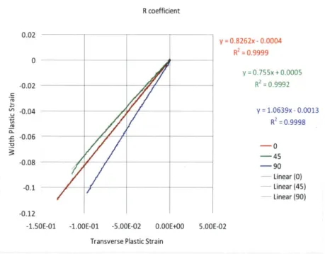
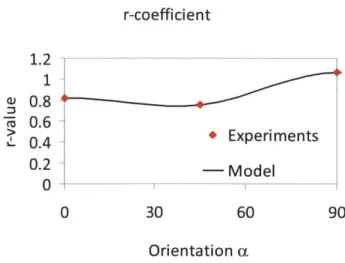
The Lankford coefficient corresponds to the slope of the curve showing the evolution of the true width strain as a function of the transverse strain. The curve has been plotted for the three specimens (Fig. 5). The fact that the Lankford parameter is not unity and not equal for all directions implies that the material is anisotropic (Fig. 6 & Table 2).
R coefficient 0.02 -0.02 6 -0.04 -c -0.06 -0.08 -0.1 -0.12
-1.50E-01 -1.OOE-01 -5.OOE-02 0.OOE+00
Transverse Plastic Strain
y = 0.8262x - 0.0004 R = 0.9999 y 0.755x + 0.0005 R 0.9992 y=1.0639x -0.0013 R2 =0.9998 -0 -45 -90 - Linear (0) - Linear (45) - Linear (90) 5.00E-02
Figure 5 Diagram of evolution of width and transverse strain for Lankford coefficients determination
r-coefficient 1.2 1 w 0.8 -F 0.6 >0.4 Experiments 0.2 0.2 - Model 0 0 30 60 90
Table 2 Lankford Coefficients Orientation a
Figure 6 According to Mohr at al. (2010), the Lankford r coefficient can be plotted as a function of the a orientation from 0 to 90 degrees,
knowing only the three coefficients in the 0, 45 and 90 degrees directions. An obvious anisotropy can be observed.
As the hardening law has only been determined experimentally in a range of strains up to the level reached at the maximum load in the uniaxial tensile test (0.2), an extrapolation is necessary to determine the mechanical behavior in a much higher range of strains.
A power law is being used in this study.
- n =
A(15)
In other words, the hardening law is written as:
H(E-) = An(gp)n~1 (16)
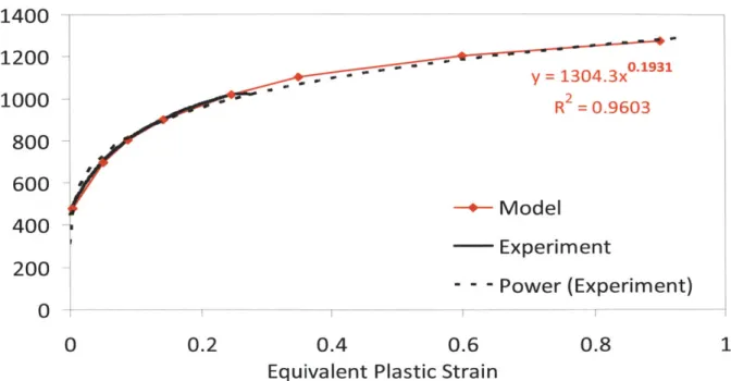
The method of least squares (in Excel: function trend line) is used to determine the two parameters of the power law before necking (Fig.7). This analytical law can be then plotted for a large range of strains. Typically, 0.9 has shown to be the maximum strain observed is this study. A discrete model is then chosen, and the points that correspond to a higher strain than that of the maximum load of uniaxial tensile tests has been adapted to fit the plasticity validation (Fig. 7 & table No. 4).
rO r45 r90
Extrapolation 1400 1200 1000 800 600 400 200 0 0.1931 y = 1304.3x R2 = 0.9603 * Model - Experiment - - - Power (Experiment) 0 0.2 0.4 0.6
Equivalent Plastic Strain
0.8
Figure 7 Interpolation, extrapolation, and discretization of the stress strain curve.
In Abaqus, the behavior of the material in the elastic range is specified by the Young modulus and Poisson ratio.
E = 200 GPa
v = 0.3
The discrete model corresponding to the power law characterizing the hardening is written in the plastic section. A potential is then added, the coefficient of which are computed from the previously determined Lankford coefficients. According to the Abaqus analysis user's manual: r (Prx + 1) R.>. = . ~~ rr
+
1)'ry(r,)
+ 1)
3(r,
+ 1)r
R(r
. R12 =2r45
+ (r.,+
ry (2r'45 + 1)(r-, + ryStress Equivalent Plastic Strain 480 0.004 695 0.05 805 0.088 900 0.141 1016 0.246 1100 0.35 1200 0.6 1250 0.9
Table 3 Yield Surface anisotropy in Abaqus
Yield surface anisotropy.
R22 R33 R12
1.067 1.0138 1.108
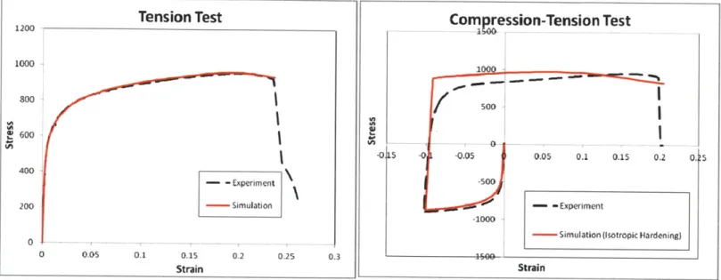
2.2 Constitutive modeling for reverse loading
The plasticity model presented above has been tested in the case of reverse loading experiments. An isotropic hardening plasticity model fails to describe the Bauschinger effect that can be observed when performing a Finite Element analysis of a test applying compression
followed by uniaxial tension to DP780 sheet metal (Fig. 8).
Com ession-Tension Test
-015 -0.05 0.05 0.1 0.15 0.2 0.!5
-500 i t
- nExperiment
-1000
- i5mulation (Isotropic Hardening)
Strain
Figure 8 Comparison of Load Displacement prediction with Isotropic Hardening in the case of linear and reverse loading
A phenomenological model is developed to describe the large deformation behavior of the advanced high strength steel under static loading. In the following, we outline the rate independent finite strain constitutive equations, which involve the yield surface, flow rule, isotropic hardening law and kinematic hardening law. Double-underscored Bold upper case letters (e.g. B) and lower case bold letters (e.g. b) are used to denote matrices and tensors, while single-underscored bold lowercase letters (e.g. b) are used to denote vectors. Square brackets are exclusively used to indicate the arguments of a function, while round and curly brackets are employed to signify the precedence of mathematical operations.
Tension Test 1200 1000 -400 - -Experiment 200 - Simulation 0 0 0.05 0.1 0.15 0.2 0.25 0.3 Strain
2.2.1 Kinematics offinite strain
The constitutive model is implemented in the commercial finite element software Abaqus/explicit. Therefore, the standard finite strain formulation for 3D elements is used (Abaqus, 2008). The Cauchy stress tensor in the current configuration is denoted as g, while d
denotes the work-conjugate strain increment. Stress and strain components, o-, and , , are
reported in the current material coordinate systems, assuming that the orthotropic material symmetry is preserved throughout loading. Formally, we write
a = Uo-(Re, 0 Rej), (17)
with R denoting the rotation of the co-rotational material coordinate system; the unit vectors e, and e2 are aligned with the initial rolling and cross-rolling directions.
2.2.2 Yield surface
The comparison of newly developed biaxial experiments (Mohr and Oswald, 2008) on advanced high strength steel sheets (dual phase steel DP590 and the TRIP-assisted steel TRIP780) with the simulation results shows that the associated orthotropic Hill (1948) plasticity model provides a satisfactory description of the large deformation response under multi-axial loading. According to C. Walters Ph.D. thesis, using the same testing technique, both Von Mises and Hill 1948 quadratic yield functions can adequately characterize the material used in this study (dual phase steel DP780) for in-plane properties, but only the Hill 1948 model was able to capture the reduction in thickness due to tensile strain.
The initial yield surface is defined as
f
=a-k=0, (18)where &= &[a_] defines the equivalent stress, k is the deformation resistance, and g is the
5 = jF(o-22 - 33)2
+
G(0-33 -01 1 )2
+H(o-l
-o-) 2 +±2L o
2 2Mo +2N U, (19)
where F, G, H, L, M, and N are the coefficients describing the material anisotropy. In the present model, we introduce a deviatoric back stress tensor a, and replace the components o in Eq. (19) by o- -e ae.
This gives the following expressions:
r-a (20)
This quadratic form can be rewritten in a matrix form thanks to the fourth order tensor operator P.
5= (g):P:(g) (21)
:= ~:P:) (22)
2.2.3Associated flow rule
An associated flow rule is chosen to describe the evolution of the plastic strain tensor.
Therefore, the increment in plastic strains, d , is proportional to the derivative of the
equivalent stress,
dcP = d2 (23)
where dA > 0 is the plastic multiplier. The integral C,
f
dA is referred to as the equivalentplastic strain.
Taking the deviatoric back stress into account and using the matrix form, the flow rule can be rewritten as follows:
d =dA ad:(24)
With:
(25)
2.2.4 Linear Kinematic hardening
The linear kinematic hardening rule is written as
2
da, =-cd, (26)
3
where cL is a material parameters. It corresponds to the linear kinematic hardening law by
Prager (1949); in this case, the back stress evolution is unbounded and evolves along the direction of the plastic strain increment.
2.2.5 Non Linear Kinematic hardening
The non-linear kinematic hardening rule is written as
da2 - d2 - c' a dA, dc (27)
2 3NLd- 2
where cNL and C2 are material parameters. This second term of the kinematic hardening
activates the dynamic-recovery term proposed by Armstrong and Frederick (1966, 2007). As a result, the evolution of the back stress is no longer unbounded and converges towards a saturation value under monotonic loading. As discussed by Lemaitre and Chaboche (1994), the dynamic recovery term may be interpreted as a description of the "fading memory effect of the
strain path." For example, in the case of uniaxial tension, the back stress evolution asymptotically approaches a saturation value.
2.2.6 Isotropic hardening
In addition to a kinematic hardening law, an isotropic hardening law is used to describe the evolution of the deformation resistance k during plastic loading. It is assumed that the deformation resistance depends on the evolution of the equivalent plastic strain. We write
dk = HAd i, (28)
where der is the increment in the equivalent plastic strain. The deformation resistance is an
exponential function of the equivalent plastic strain,
k = ko + H0 1-exp[-A zP]}, (29)
with the model parameters ko, HO , and A. Consequently, the relationship for the isotropic strain hardening modulus reads
dk
H,[6'1= = AHo exp[-Az' ].
dZsP (30)
2.2.7 Plasticity modelparameter identification
The Calibration of the Hill surface is performed by measuring the lankford coefficients characterizing the anisotropy of the material.
The initial yield point ko has been found to be different in compression and tension. Therefore an initial back stress has to be determined to take this asymmetry into account, and ko is taken as the average of the yield point in tension Y, and the yield point in compression Y2 .
According to Beese and Mohr (2011), the back stress induced by the rolling procedure should have the following form:
a 0 0
=
0 0
.
(31)
0 0
-a-The tensor is written so that the first direction corresponds to the rolling direction, and the third to the through thickness direction.
The main goal of the numeric model is to be able to predict the stress and strain state up to fracture at the fracture locus. Therefore, the behavior of the material must remain accurately predicted after the onset of the necking phase. It is not possible to determine experimentally suitable values for the plasticity model parameters that allow us to predict the load displacement relation after the onset of the necking phase. In these conditions, the calibration of the IH + LK + NLK hardening model, using 5 parameters, requires us to use an optimization method.
An order of magnitude for the parameters can be estimated by looking at the asymptotic behavior of the material at very large deformation.
Alternatively, a simplified 1 D model for uniaxial tests is first implemented in order to have a first guess on the seeds values for the modified Yoshida model. The computationally efficient method allows us to use a Monte Carlo method to look for the coefficients. For each parameter in the model, a certain domain delimited in a minimum and a maximum possible value is guessed, according to the expected result. The load displacement predicted by the ID model is compared to the experimental load displacement relation for each compression tension test. This comparison can only be done up to the point corresponding to maximum load, as the 1D model becomes irrelevant after the onset of diffused necking. The set of parameters which minimizes the area between the experimental and predicted stress strain curve is kept as seed values for the main optimization procedure.
In order to carefully optimize the parameters of the plasticity model, an inverse calibration using Finite Element Analysis is performed. In order to determine a suitable set of parameters, an objective function defined by the error between the experimental and numerically predicted load displacement relation is introduced.
[C,y,
H,Q,
b] = arg mincrHQb JFFEA(u) - FEXP(u) (32)Tests
This is an unconstrained non-linear optimization problem that can be solved using a derivative-free simplex algorithm. To solve this problem, the Matlab function "fminsearch" has been used. This function uses the Nelder-Mead method described by Lagarias et al. (1998). It requires introducing a coupling with Finite Element software (Abaqus) in order to be able to evaluate the objective function at each step of the optimization process.
2.3 Identification of the load path to fracture
Macroscopic ductile fracture models are based on a damage accumulation during the loading history. Bai and Wierzbicki (2008) conclude that this damage accumulation shows great dependency on some parameters of the stress state. The history of two stress invariants, triaxiality and Lode angle, play a major role.
2.3.1 Stress and Strain invariants
The Equivalent Plastic Strain 01 is defined by:
t EgP = PI + ftPldt
where Po is the Initial Plastic Strain.
The strain rate Pi being:
Triaxiality i7 is by definition:
-p q
With the pressure p, Von Mises stress q and deviatoric stress s are calculated as shown:
p = o-ii = tr (a) q = (s: s)
s = p=)
(33)
Triaxiality can be understood as a normalized pressure. It describes the average level of the stress and its distribution along the three principal directions.
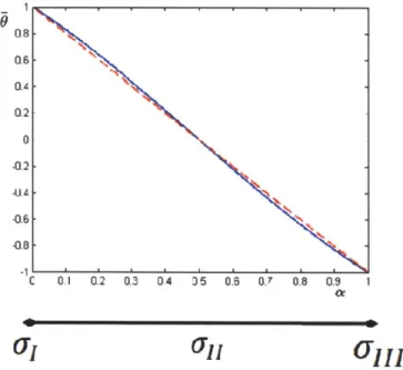
The dimensionless Lode Angle parameter is defined by:
= 1-- arccos(() (34)
with ( being:
r3
(35)
A coefficient a is now introduced:
a I - (36)
In other words, a is the relative position of the second principal stress between the two others. The Lode Angle is a function of a only:
6 = 6(a) (37)
According to the graph showing 6 as a function of a (Fig. 10), 6 can be approximated with good accuracy thanks to the following formula:
The Lode angle must be interpreted as an indicator of the relative position of the second principal stress between the two other ones (Fig. 9).
0.5 0V 0.8 0.9
(7,
III
Figure 9 Interpretation of the Lode Angle in terms of principal stresses.
2.3.2 Modified Mohr Coulomb Model for
fracture
The previous results indicate that a criterion to predict the fracture must take into account the history of the stress state during the loading.
Bai and Wierzbicki (2008) have modified the Mohr Coulomb criterion (MMC) to predict the fracture with a damage accumulation that takes the history of the state of stress into account. The fracture locus for proportional loading is defined as:
s
=
A
[C
3+
(1
C3)
(sec
-
1
cos
(+
ci
+ sin
(
For non-proportional loading, linear incremental form of damage indicator D is:
r-P
D(E")
The fracture initiates when:
D (lf) = 1
It will be useful later in this study to introduce the plane stress 36 ondition -3 3 = 0 n
(Wierzbicki, Xue, 2005):
sin(
0)
2
(42) where:f
=
cos
{arcsin
-
2(2
(43)F1+c-(40) (41) U =
f
c + 3 (44) (45)_f
q50
27-
22 q
7 t 2isin -1arcsin
-
(-2-fA = C3 + 1- c 3)( 1 0
2 -O r3f
Chapter 3.
III Fracture experiments
3.1 Experiments
3.1.1 Specimens
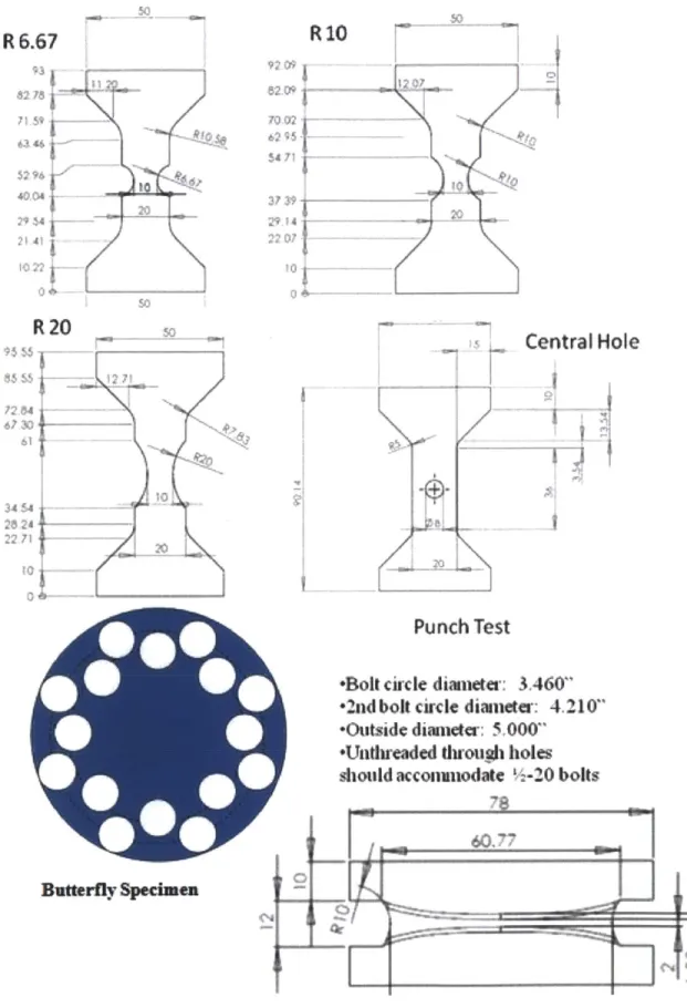
Several different specimens are tested in order to study the fracture in a large range of states of stress both in terms of triaxiality and Lode angle. Various shapes of specimens for testing in a tensile machine are used because they are easy to perform and require universal testing equipment that is available in the industry. Notched specimens are used because the location of the onset of fracture always is know a priori (where the width is the smallest) and various histories of triaxiality and Lode angle can be studied by designing different notch radii. The central hole specimen allows to keep an almost constant type of loading, very close to uniaxial tension, all the way to fracture, whereas the triaxiality of the notched tensile specimens always shift at a certain point to a value close to that of biaxial tension, depending on the radius.
The punch test presents an equibiaxial loading and is the only test that allows us to observe a negative Lode angle. requires two video cameras and calibration to observe the displacement in the 3D space. The shear test, performed thanks to the butterfly specimen, is also interesting, as it is the only test that shows triaxiality close to zero. It has been performed on a biaxial hydraulic Instron machine, using a 200kN load cell in the vertical direction and a 25kN load cell in the horizontal direction. A zero force loading in maintained on the tensile direction, and shear loading is imposed on the horizontal direction. In fact, central hole and shear tests are the only ones where fracture does not occur on a triaxiality close to 0.66, so they have critical importance to determine the effect of triaxiality on fracture.
Various types of specimens, that allow us to reach a large range of loading histories all the way to fracture, are needed to be able to observe a dependency of the fracture locus on the type of loading and state of stress. (Fig. 10)
R 6.67 RIO 179 5e9 70 2 29
i
I
R 20 Central Hole 0-_-Punch Test
+*Bolt
circle dia-neter: 3.460"
-2nd bolt circle dianeter: 4.210"
-Outside diander: 5.00"
*Unthreaded drough holesshould acconuodate
--
20 bolts
78 60
Butterfly Seie
3.1.2 Digital Image Correlation
In this study, numeric simulation is used to determine local stress state and the local strains in the experiments. A comparison between the experiment and the simulation must be done to make sure that the simulation exactly describes the experiment. To do so, Load Displacement curves are compared. It would be too complicated to take into account the mechanical behavior of all the devices that interfere with the displacement measured by the tensile machine. That is why displacement measurements are made on the surface of the specimen itself, using the Digital Image Correlation (DIC), assuming that there is no dependency of the displacement in the depth of the specimen.
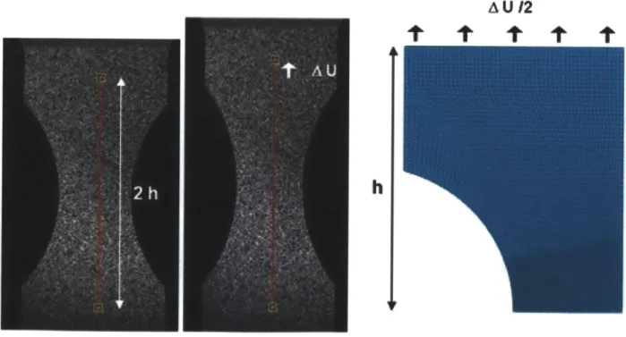
Virtual extensometers are used to measure the relative displacement between two points symmetrically opposed to the center of the specimen. The mesh is designed so that its boundaries have the same position as the extensometers extremities. Thus the measured displacement is imposed as the boundary limit in the simulation (Fig. 11). It has previously been verified that the displacement is constant along the width of the specimen at that position.
A U 12
t t t t t
2
h
h
Figure 11 Displacement measured by Digital Image Correlation using extensometer and the corresponding Finite 39 Element Model
The onset of fracture is determined thanks to DIC. The fracture occurs between the last picture where no crack can be seen and the following picture, where a macroscopic discontinuity in the material is observed (Fig. 12). The uncertainty in the exact time when fracture first occurs is exactly the amount of time that separate two successive images. The consequence in the error in displacement is shown in the plasticity validation section.
tlBs
rai=1s
Figure 12 On the left: last picture before the onset of fracture. On the right: first picture after fracture.
3.2 Computational Model
3.2.1 Finite Element Model
Implicit finite element simulations are performed for each experiment using Abaqus/standard. According to Mohr and Dunand (2010), solid elements should be preferred to shell elements. Reduced-integration eightnode 3D solid elements (type C3D8R of the Abaqus element library) are used to mesh the specimens. The mesh size has a very strong impact on the results. A fine mesh is required in the location when localized necking occurs to provide satisfying convergence of the results. That is why a certain type of mesh adapted to the geometry of the specimen is used. The mesh size is dramatically refined in the area of necking. According
to the study on the mesh size effect by Mohr and Dunand (2010), a mesh size of 0.1mm per element should be used, providing a good compromise between computation time and accuracy with 0.2% of variation with the result where the mesh size is doubled. The time step is also chosen so that good accuracy is reached. It is also taken advantage in the finite element model of the different symmetries of the problem to decrease the computing time (Fig.13). To be more specific, only one eighth of the specimen is modeled (the upper left quarter of the specimen, with half its thickness), thanks to three planes of symmetry. in the Abaqus code, zero-normal displacement and zero in plane rotation conditions are imposed on the nodes included in each plane of symmetry.
3.2.2 Fracture Locus
Simulations of the experiments are performed to observe the history of triaxiality, Lode angle and strain in the element where fracture first occurs. In order to find out which element corresponds to fracture initiation locus, it is assumed that the fracture location corresponds to the element with the highest equivalent plastic strain.
In the case of the notch specimen, it can be observed from the Finite Element simulation that the point that has the highest equivalent plastic strain at the instant of fracture is right in the middle of the specimen, in terms of thickness, height and width (Fig. 14). It is a little bit different with the central hole specimen, as it seems that the element is not in the border of the hole as expected, but a little bit inside, though it is still in the middle in terms of thickness and height. In the case of the punch test, it is in the middle of the specimen. The strain is rather constant over a wide area in the butterfly specimen.
Figure 14 Guess on the position of the element corresponding to the location of the onset of fracture for each specimen mesh.
In order to determine the instant corresponding to the fracture in the simulation, AU is defined as the displacement observed with the extensometer and DIC at the moment of the fracture. Triaxiality, equivalent plastic strain and Lode angle at fracture are determined when the displacement in the simulation reaches AU (Fig. 15). As AU falls between two steps of the simulation, a linear interpolation between the values at the previous step and next step is performed.
R
10
:
Force/Displacement Curve
Identification of fracture
1.2 .1G I o0.8 a.0.6 S0.4 LLI 0.2 0.5 A U/2 1 Displacement (mm) 3 1 2 3 Displacement(mm)AU
Figure 15 On the left, force versus displacement curve and displacement at fracture. On the right, strain as a function of the displacement and strain at fracture determined by the measured displacement at fracture.
In the case of the punch test, the displacement at fracture in unknown, that is why the reduced thickness of the sheet at the point of fracture tf is measured to determine the strain and state of
stress at fracture in the simulation (Fig. 16).
E
=
in
(
Identification of fracture
. Equivalent plastic strain
at fracture
-Simulation
(46)
Thickness at fracture (from experiment and direct measurement)
Figure 16 Strain as a function of the thickness in the case of the punch test and strain at fracture determined by the measured thickness at fracture.
3.3 Results
3.3.1 Plasticity Validation
Force-displacement curves obtained by experimental measurements and computer simulation are here compared to decide whether simulation is likely to give a good prediction of the stress state or not. It is assumed that the simulation reaches a good accuracy when the energy corresponding to the gap between the two curves is negligible. It is here visually concluded that the R6.67 notch specimen and butterfly specimen are the only cases where experimental and computational results do not match with satisfaction, as the loading force is overestimated. It must be noted that divergence happens in a range of strains where the maximum load has not yet been reached in the uniaxial test, suggesting that the Hill 1948 model of the behavior of the material itself is responsible for the error, more than an uncertainty in the determination of the hardening law.
In the case of the punch test, DIC has not been performed. This explains why there is not a good prediction of the simulation in terms of load and displacement. Simulation does not take into account the behavior of all the devices located between the specimen itself and the displacement measurement. It confirms the idea that DIC is necessary to determine the displacements in the specimen. On the other hand, a very good level of prediction can be reached if considering the time scale instead of the displacement. It is here supposed to be enough to validate the method.
It can be observed that the uncertainty of the onset of fracture in time leads to an error of 1% in the displacement. However, it corresponds to the point where load falls to zero within the same range of error.
Next two pages: Fig. 17 Comparison of experimental and computer predicted Force displacement curves and fracture locus.
R6.67: Force/Displacement Curve 14 10 aIC LL. 4 -- Experiment 2 - Simulation 0 , I , , , , | 1 , , , I i , , , 1 1 , I , I 0 0.5 1 1.5 2 2.5 Displacement (mm)
R 10 Force/Displacement Curve
14 12 10 z 8 L_ 6 LL 4 -Experiment 2 -Simulation 0 0 1 2 3 Displacement(mm) R 20 Force/Displacement Curve 14 12 10 8 6 U - FxperimentI 2 -Simulation 0 1 0 1 2 3 Displacement(mm)R6.67: Force/Displacement Curve
13 12.5 12 z 11.5 -- Experiment 0 11 - Simulation 10.5 -- Fracture 10 1.8 2 2.2 2.4 2.6 Displacement (mm)R 10 Force/Displacement Curve
12.7 12.5 -- Experiment -Simulation 12.3 -+-Fracture w12.1 0 U-. 11.9 11.7 11.5 , , , , , I 2.2 2.4 2.6 Displacement(mm) R 20 Force/Displacement Curve 12.2 -Fxperiment 12 -Simulation 11.8 -4--Fracture 11.6 U o 11.4 11.2 11 10.8 3.4 3.5 3.1 3.2 3.3 Disolace-nent(mm)Figure 17 Comparison of experimental and computer predicted Force displacement curves and fracture locus
Central Hole: Force/Displacement
16.00 CurvMe 14.00 12.00 -10.00 aU 8.00 U 0 u- 6.00 4.00 - Experiment 2.00 - Simulation 0 .00 , . , , , , . , , , 1 0.00 0.50 1.00 1.50 2.00 2.50 Displacement(mm)
Central Hole : Force/Displacement Curve
14.50 14.40 - Experiment 14.30 14.20 -Simulation Z14.10 au14.00 -+-Fracture U 013.90 13.80 13.70 13.60 13.50 1.90 2.00 2.10 2.20 2.30 Displacement(mm)
Butterfly: Force/Displacement curve
25 20 S15 10 - Experiment --- Simulation 5 *-Fracture 0 0 0.5 1 1.5 2 2.5 3 Displacement (mm)
Experimentvs Simulation: Disp/Time
120 100 ---- 1l'och_1 80 40 20 0 0.2 0.4 0.6 0.8 1 1.2 Time
Experiment vs Simulation: Disp/Load 120 100 80 --- ='unch2 -- Sirrulation 60 -J40 20 01 0 15 10 lb 2C b Cispla-.er-e-t (mmr)
3.3.2 Results
The evolution of the triaxiality and the Lode angle and the values at fracture can now be observed for each specimen (Fig. 18). The uncertainty in time of fracture is shown on the graphs. For a study of experimental and numerical error please refer to Dunand & Mohr (2010).
The stress state varies a lot during the loading for the notched specimens. The stress of state also varies, but in smaller proportions for the central hole specimen, whereas it is constant with the shear test. In the case of the punch test, the variations at the beginning of the loading are more probably due to errors in the computer model. The equivalent plastic strain at fracture is different for each of these tests. It is also true for the different notched specimens, even if the
stress state at fracture is almost the same in each case.
Strain-Triaxiality hisLIory _ Bulletfly . 0.0 R67 0.7 o 0.6 -Punc-Tst # 0.5 1 N: 0.4 -Central Hole cu 0.3 > 0.2 - R10 ' 0.1 + frracture C -min 0 0.2 0.4 0.6 0.0 Fituctuie Triaxiality max
Strain-Lode historv
1.2 C.8 C.6 C.4 C.2 0 -0.E -Butterfly - Central Hole * Fracture mh + Fracture IJ1HX -- Pujn::h Te -l -R667 - R10 C.5 0 Lodo /\nqlc3.3.3 Identification of the MMC parameters
To determine the three parameters c1, c2, c3 of the Modified Mohr Coulomb criterion that best fits the material, an inverse calibration is done. The method of least squares is used to minimize the distance of the damage at fracture in the simulation to unity for each experiment:
N
[c, c2, ca -3 ag min (1-_D (r/, U,))2 (47)
1
(N is the number of experiments)
A Matlab program using the function fmincon looks for local minima in a space specified by the lower and upper limits for cI, c2, c3. More specifically, the function looks for the closest local minimum to a solution guessed by the user. The method is in fact very unstable, and the results vary a lot depending on the initial value.
To have a good first guess on the parameters, a simpler problem must be considered. That is why the plane stress condition is first assumed to be true. It allows us to solve the equation in a 2D plane instead of a 3D space. In addition, to avoid the inverse problem, it is assumed that the damage function is constant during the loading. If 'q and 0 are constant during the loading, then the equations reduce to:
E
= f(77f,
56) ,s(7f
, Of) = 1 (48) The optimization problem reduces to:N
[cI,
c
2, c3]g minci
ec2,c3
Zf(0 7,
0))2
(49)i=1
and its solution yields:
[c1, c2, c3] = [0.06676, 676.6, 0.9503] (49)
Using the above values as initial conditions, the 3D inverse method gives:
The results of the calibration are plotted on Fig. 19 & 20.
~1.2--0
Pu ch test
0.8Shear test
... 4... ...hd
C0.
--Notched
W 0 -0.5 0 0.5Stress triaxiality
Figure 19 Fracture locus in terms of strain as a function of the triaxiality with the hypothesis of plane strain, and fracture locus of
the experiments. Shear
tes-nch test'
1tral hole
tr L1
.1
-Figure 20 A plot of the full modified Mohr Coulomb criterion. Strain at fracture is a function of Lode angle and triaxiality.
3.3.4 Validation of the model
To compare the prediction of the fracture model to the experiment, the experimental displacement at fracture and the strain are compared to the displacement and strain predicted by the simulation where the damage accumulation reaches 1 (Fig. 21).
AUnumn(ff) =?AUf (51)
This is shown in Fig. 21. For each specimen: On the left: damage versus displacement curve with damage and displacement at fracture, and predicted displacement at fracture when damage equals one.
On the right: damage versus strain curve with damage and strain at fracture, and predicted displacement at fracture when damage equals one.
R6.67: Damage accumulation
1.2 3.8 I 3.4 Ii Ii 3.2 )amage -- 4 periment II 0 0 0.5 1 1.5 DisplacementRIO: Damage accumulation
1.2 1--- -<_mwI 0.8 E 0.6 0.4 -- Damage 0.2 - Experiment 0 0 0.1 0.2 0.3 0.4 0.5 0.6 0.
Equivalent Plastic Strain
R20: Damage accumulation
1.2 1 0.8 10.6 0.4 0.2 0R6.67: Damage accumulation
2 1 8 4 6 I I 4 I 2 4Damage 2 1 -LExperiment 0 0 0.1 0.2 0.3 0.4 0.5 0.6 CEquivalent Plastic Strain
RIO: Damage accumulation
--- "" "" - " "" I SDamage - E::periment 0.2 0.4 0.6 08 1 1.2 1.4 Displacement
R20: Damage accumulation
1.2 1 0.8 0.6 0.4 0.2 0 1 Displacement 0.2 0.4 0.6Equivalent Plastic Strain
1.2 1 0.8 0.6 0.4 0.2 0 0 --- I1 I --Darnag 1.5 51