HAL Id: hal-00318397
https://hal.archives-ouvertes.fr/hal-00318397
Submitted on 6 Nov 2007
HAL is a multi-disciplinary open access
archive for the deposit and dissemination of
sci-entific research documents, whether they are
pub-lished or not. The documents may come from
teaching and research institutions in France or
abroad, or from public or private research centers.
L’archive ouverte pluridisciplinaire HAL, est
destinée au dépôt et à la diffusion de documents
scientifiques de niveau recherche, publiés ou non,
émanant des établissements d’enseignement et de
recherche français ou étrangers, des laboratoires
publics ou privés.
atmosphere at solar minimum from global circulation
model simulations
T. Moffat-Griffin, A. D. Aylward, W. Nicholson
To cite this version:
T. Moffat-Griffin, A. D. Aylward, W. Nicholson. Thermal structure and dynamics of the Martian
upper atmosphere at solar minimum from global circulation model simulations. Annales Geophysicae,
European Geosciences Union, 2007, 25 (10), pp.2147-2158. �hal-00318397�
www.ann-geophys.net/25/2147/2007/ © European Geosciences Union 2007
Annales
Geophysicae
Thermal structure and dynamics of the Martian upper atmosphere
at solar minimum from global circulation model simulations
T. Moffat-Griffin1,*, A. D. Aylward1, and W. Nicholson1
1Atmospheric Physics Lab, University College London, UK *now at: British Antarctic Survey, Cambridge, UK
Received: 2 February 2007 – Revised: 13 September 2007 – Accepted: 18 October 2007 – Published: 6 November 2007
Abstract. Simulations of the Martian upper atmosphere have
been produced from a self-consistent three-dimensional nu-merical model of the Martian thermosphere and ionosphere, called MarTIM. It covers an altitude range of 60 km to the upper thermosphere, usually at least 250 km altitude. A ra-diation scheme is included that allows the main sources of energy input, EUV/UV and IR absorption by CO2and CO,
to be calculated. CO2, N2 and O are treated as the major
gases in MarTIM, and are mutually diffused (though neu-tral chemistry is ignored). The densities of other species (the minor gases), CO, Ar, O2 and NO, are based on diffusive
equilibrium above the turbopause. The ionosphere is cal-culated from a simple photoionisation and charge exchange routine though in this paper we will only consider the ther-mal and dynamic structure of the neutral atmosphere at so-lar minimum conditions. The semi-diurnal (2,2) migrating tide, introduced at MarTIM’s lower boundary, affects the dy-namics up to 130 km. The Mars Climate Database (Lewis et al., 2001) can be used as a lower boundary in MarTIM. The effect of this is to increase wind speeds in the thermo-sphere and to produce small-scale structures throughout the thermosphere. Temperature profiles are in good agreement with Pathfinder results. Wind velocities are slightly lower compared to analysis of MGS accelerometer data (Withers, 2003). The novel step-by-step approach of adding in new features to MarTIM has resulted in further understanding of the drivers of the Martian thermosphere.
Keywords. History of geophysics (Atmospheric sciences;
Planetology) – Ionosphere (Planetary ionospheres) – Atmo-spheric composition and structure (Aerosols and particles)
Correspondence to: A. D. Aylward (alan@apl.ucl.ac.uk)
1 Introduction
Mars is the fourth planet from the Sun and has a radius of 3397 km, around half the size of Earth. The presence of a ten-uous atmosphere on Mars was suggested by Herschel as early as 1784, though his observations of changes in “clouds and vapours” were possibly based on telescopic artifacts. The exact composition of the atmosphere was still causing de-bate into the early half of the 20th century. The first robotic fly-bys (the Mariner and Mars missions) of Mars in the late 1960s provided definitive measurements of the atmospheric composition and atmospheric pressure, showing a low pres-sure, CO2 dominated Martian atmosphere. The Viking
or-biter and lander program in 1976 added further limited data on the atmospheric neutral and ion densities, pressure and temperature being collected as the landers passed through the atmosphere (Nier and McElroy, 1977; Hanson et al., 1977). This was to remain the main dataset for the Martian atmosphere for almost two decades before the arrival of the Pathfinder mission in 1997 heralded an expansion in Mars exploration.
One-dimensional models of the Martian atmosphere (Bougher and Dickinson, 1988) have been used to exam-ine the physical processes that determexam-ine parameters such as temperature in an effort to match to the data measured by the early missions. To better understand the dynamics and energetics of the Martian atmosphere, three-dimensional global circulation models (GCMs) were developed (Bougher and Dickinson, 1990; Forget et al., 1999). In developing a new model the aim has been to further understanding of the drivers of the Martian thermosphere. A step-by-step ap-proach enables the corresponding changes seen in the ther-mosphere to be associated with each new feature added, e.g. the effect of IR heating and cooling on the thermosphere. It is the results from this approach that this paper deals with.
Below, in Sect. 2 the UCL Martian Thermosphere Iono-sphere Model (MarTIM), is described. Sections 3 and 4
cover the basic model results for EUV solar forcing and EUV and IR solar forcing, while Sects. 5 and 6 examine the effects on MarTIM of including tides and coupling to a lower atmo-sphere model, respectively. Comparisons between MarTIM and data are examined in Sect. 7.
2 The model
2.1 Basic model features
MarTIM, is a global three-dimensional numerical model of the Martian thermosphere and ionosphere above a pressure level of 0.883 Pa – an average altitude of 60 km. This pres-sure has been chosen as it is thought to be above the influ-ence of the dust storms that can cover the planet (Peters, 2001). It is also below the turbopause and includes the main region of infrared LTE and non-LTE heating and cooling. MarTIM uses the same mathematical formulations as the Ti-tan thermosphere GCM (Mueller-Wodarg, 2000), eliminat-ing the need to recode the main model equations for Mars. It also means that MarTIM’s setup and output format match existing thermospheric GCMs at UCL (Smith et al., 2005), aiding decoding and sharing of visualisation programs. The co-ordinate system in the model is an Eulerian co-rotating pressure grid. MarTIM divides the atmosphere by latitude, longitude and pressure level, forming cells. These have vari-able resolution in the three spatial dimensions. For each cell the energy, momentum and continuity equations are solved for each timestep, which is typically 10 min. The model can be started either from a one-dimensional set of parameter profiles or from the output of a previous model run. If run to steady state (repeating the same conditions for multiple days) it takes typically four model days to reach steady state. The model can also be timestepped to reproduce day-to-day variability.
The thermosphere modelled by MarTIM is described by seven constituents – CO2, N2, O, Ar, NO, O2and CO. The
major constituents, CO2, N2 and O are mutually diffused.
All neutral densities are initially read in as globally averaged 1-D model profiles, based on Viking Lander solar conditions. As yet, the model does not consider the neutral chemistry, its variations over the globe and its feedback on thermal struc-ture and dynamics. Up to the turbopause (around 125 km), the number densities of the constituents remain in fixed pro-portions as they are turbulently mixed. Above this, they are molecularly mixed and their densities fall off in proportion to their mass. Despite the similar densities of Ar and CO at the turbopause, O is classed as a major constituent. In the Martian atmosphere the ratio of O to CO2 has a
ma-jor influence on the vertical distribution of infrared cooling (Lopez-Valverde and Lopez-Puertas, 2001). This effect is greater than the effect of CO on infrared heating. The num-ber of major constituents chosen was restricted to three due to the method of calculating diffusion (Fuller-Rowell, 1981),
where the number of terms in the diffusion equation increase by n!, where n is the number of species involved, resulting in increased complexity and model run time. The minor con-stituent profiles are assumed constant up to the turbopause and then fall off with their own scale heights.
In the first MarTIM runs considered the only energy source comes from heating through solar EUV and IR ab-sorption. The solar radiation penetration scheme (Mueller-Wodarg, 2000) calculates the absorption of EUV radiation in the range 0.2–172.5 nm throughout the whole thermo-sphere. Work done with another Mars GCM, comparing with contemporaneous temperature data (Bougher and Dickinson, 1988), concluded that the solar EUV radiation heating effi-ciency (the amount of absorbed radiation that contributes to heating) is in the range 15–20% for Mars. Similar consid-erations have lead to MarTIM using a value of 18% for the heating efficiency (Moffat, 2005).
Absorption and emission in the near infrared (IR) bands of CO2and CO becomes important for atmospheric heating and
cooling above 50 km, and is dominant in the middle atmo-sphere of Mars (i.e. the region from the lower boundary to the turbopause). Equations exist that can calculate the amount of heating and cooling due to IR radiation. The departure from local thermodynamic equilibrium (Lopez-Puertas and Lopez-Valverde, 1995) above 80 km on Mars adds complex-ity to the calculations. The full IR calculations, if imple-mented in MarTIM, would slow down the model calculations to unacceptable levels. Parameterised versions of the calcula-tions, accurate to 1–2% (Lopez-Valverde and Lopez-Puertas, 2001) are implemented in MarTIM.
A basic photochemically determined ionosphere is also in-cluded in MarTIM, with photoionisation and ionic reactions occurring above 80 km used to determine the ion and electron density distributions. Ion diffusion is predicted to take over from photochemistry above 170 km (Mahajan and Dwivedi, 2004). The model is expected to be accurate up to this alti-tude but differ slightly from expected ion densities above it. We will not discuss the ionospheric results in detail in this paperi because they do not affect the derived neutral temper-atures and winds.
Martian seasons are measured in this paper according to Solar longitude – the angle between the Mars-Sun line and the Martian line of equinoxes. Ls=0◦ corresponds to
the spring equinox in the Northern Hemisphere of Mars.
Ls=180◦is autumn equinox in the Northern Hemisphere. All
MarTIM simulations are for season Ls=0◦ and solar
mini-mum conditions, unless stated otherwise. The MarTIM sim-ulations for this paper are at a vertical resolution of half a scale height and a horizontal resolution of 6◦by 6◦latitude and longitude. This is with the exception of the final re-sults section where the latitude and longitude resolution is set to 5◦, to match the horizontal resolution of the lower at-mosphere model.
2.2 Equations
The three-dimensional momentum and energy equations in Eulerian space are given by Eqs. (1) and (2), respectively (Mueller-Wodarg, 1997). ∂V ∂t = −V ·∇pV −ω ∂V ∂P−∇p8−(2+ Vy R cos θ)k×V +g ∂ ∂P µ HP ∂V ∂P + 1 ρµ∇ 2 pV (1)
The terms on the right side of Eq. (1) represent respectively the advection, curvature forces, pressure gradient, the Corio-lis force and the vertical and horizontal viscosity. Individual terms are defined in the appendix.
∂ǫ ∂t =QEU V +I R+QCO2− V · ∇(ǫ + gh) − ω ∂(ǫ + gh) ∂P +V ·g ∂ ∂P µ HP ∂ ∂PV + 1 ρ(KT +Km)∇ 2T +g ∂ ∂P (KT +Km) H P ∂T ∂P −g ∂ ∂P KTg cP (2)
The terms on the right hand side of the equation are the heat-ing due to Solar EUV and IR radiation, the coolheat-ing due to IR emission, the horizontal energy transport, the adiabatic heating and vertical energy transport, viscous heating and the horizontal and vertical heat conduction terms.
The IR heating parameterisation used has been developed from work done at the Instituto do Astrofisica de Adalu-cia (IAA), Spain (Lopez-Puertas and Lopez-Valverde, 1995), with CO2 absorbing radiation at 4.3 µm and 2.7 µm
wave-lengths. The IR cooling parameterisation equation (Lopez-Valverde and Lopez-Puertas, 2001), used in MarTIM, is from the IAA. Equations (3) to (5) explain the calculation of the IR cooling rate in terms of 15 µm IR emission by CO2.
Q15µm(z∗) = −hc β 4[v1A1T1(z ∗, ∞)n∗ 1 +v2A2T2(z∗, ∞)n∗2] (3)
Where Q15 µm(z∗) is the IR cooling rate at a height z∗, h is Planck’s constant, c the speed of light, n∗
1,2are the
popula-tions of the excited states, T the flux transmission to space, β the diffusivity factor (=1.8), A the Einstein coefficient and v the wavenumber of the band.
The populations of the excited states are calculated using Eqs. (4) and (5) (Lopez-Valverde and Lopez-Puertas, 2001).
n∗2=l1P2+α2P1p21 l1l2−p12p21 (4) n∗1=P1 l1 +α1 n2p12 l1 n∗2 (5)
where Pn is the collisional production of state n from all
Vibrational-Translational (V-T) processes (Lopez-Valverde and Lopez-Puertas, 2001), pnmis the collisional production
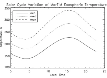
Fig. 1. Thermospheric (pressure=2.7×10⁻⁷Pa) temperature varia-tion, from MarTIM, Ls=0◦, for solar minimum, medium and
max-imum conditions, along the equator over a day.
of state n via Vibrational-Vibrational (V-V) exchange from the (010) state of isotope m, lnis the collisional loses of state
n from all V-T and V-V processes in which it participates. α is a combination of the Einstein spontaneous emission coef-ficients for the strong and weak bands, the velocity of light and the Planck constant (Lopez-Valverde and Lopez-Puertas, 2001).
The V-T reaction between O and CO2is one of the main
reactions that control the distribution of the cooling height profile. The V-T rate coefficient used in MarTIM is set to 1.×10−19m3s−1. This rate coefficient for MarTIM, which
is slightly lower than for other Mars models (Angelats i Coll et al., 2004), was determined using heat balance work (Bougher and Dickinson, 1988; Moffat, 2005) and compar-isons with cooling profiles in the literature (Bougher and Dickinson, 1988; Lopez-Puertas and Lopez-Valverde, 1995).
3 Basic model results
3.1 Diurnal and seasonal variations in temperature
The main EUV heating occurs in the Martian thermo-sphere between 1.2×10⁻⁹Pa and 2.4×10⁻⁴Pa pressure lev-els (140 km to 250 km for Solar minimum conditions). As the EUV solar flux varies over the solar cycle this will cause a corresponding variation in thermospheric temperatures. Fig-ure 1 illustrates MarTIM thermospheric temperatFig-ure results for Solar minimum, medium and maximum conditions.
The thermospheric temperatures in Fig. 1 show the ex-pected increase in temperature with increase in solar activity. The peak daytime variation of 115 K over the solar cycle for
Ls=0◦is consistent with other basic GCM results (Bougher
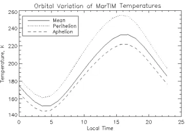
Fig. 2. Thermospheric (pressure=2.7×10⁻⁷Pa) temperature varia-tions, from MarTIM, for solar minimum condivaria-tions, for perihelion, aphelion and mean orbital positions, along the equator over a day.
Solar flux variation also occurs due to the ellipticity of Mars’ orbit. The solar flux can vary by 40% over the course of a Martian year. The EUV flux variation due to orbital position, although smaller than most of the solar cycle vari-ation, would be expected to have an effect on the thermo-spheric temperatures. Simulations, at constant solar activity were performed with MarTIM for different orbital positions. A response to the seasonal variation is seen in Fig. 2, with the thermospheric temperature being higher at perihe-lion (greater flux) than apheperihe-lion (lower flux). The overall seasonal variation in peak temperature variation is 45 K, a significant amount.
3.2 Neutral structure
Neutral constituent densities are defined at the start of a model simulation. There is no neutral-neutral chemistry within MarTIM at this stage, but there is diffusion of the ma-jor species. Figure 3 shows the initial O:CO2number
den-sity ratio compared to the height profiles of the same ratio at 05:00 local solar time and 15:00 local solar time after the model has run to steady state. Figure 3 also shows the same ratio , for the same conditions as MarTIM, produced by MT-GCM (Bougher, 2007b), a Mars MT-GCM developed in the U.S.
4 Non-LTE IR heating and cooling
In the Martian middle atmosphere the energy balance is con-trolled by CO2non-local thermodynamic equilibrium
(non-LTE) effects (Lopez-Puertas and Lopez-Valverde, 1995). Descriptions of non-LTE effects in the atmosphere can be found in Puertas and Taylor (2001) and Lopez-Valverde (1998).
[O]/[CO2] Number Density Percentage Ratio
0.0 16.7 33.3 50.0 66.7 83.3 100.0 [O]/[CO2] 60 80 100 120 140 160 180 Height (km)
Fig. 3. O:CO2 neutral number density ratio profiles at Ls=90◦,
from MarTIM (black lines) and MTGCM (blue lines) (Bougher, 2007b), for 15:00 LST (solid lines) and 05:00 LST (dashed lines) at the equator. The solid red line is the MarTIM initial ratio.
Parameterisations of the full non-LTE calculations, that are accurate to within a few percent compared to the full calculation (Lopez-Valverde and Lopez-Puertas, 2001), are used in MarTIM.
The incorporation of IR heating and cooling schemes into MarTIM altered the structure of the high altitude tempera-ture distributions compared with the basic simulations. Fig-ure 4 compares the same pressFig-ure level for EUV/UV and EUV/UV+IR simulations for solar minimum, Ls=0◦, with
differences in structure as well as absolute values apparent. The drop in average temperature across the pressure level, seen in the top image in Fig. 4, is part of a general at-mospheric cooling (note the mean lower altitude of the EUV/UV+IR simulation pressure level) and is caused by a stronger dayside upwelling in the vertical winds along the equator. This affects the divergence winds and causes stronger adiabatic cooling on the equator, affecting the peak afternoon heating . The temperature range is 60 K across the top plot and 90 K across the bottom plot. A similar structure has been seen in some Mars modelling work (Bougher and Dickinson, 1988), but has not been highlighted by other Mars models. This highlights the need for a step-by-step approach
Fig. 4. Pressure level 30 (pressure=2.7×10⁻⁷Pa) temperature plots for EUV/UV and IR forcing (top) and EUV/UV only forcing (bot-tom), for solar minimum, Ls=0◦.
to understand the underlying features of the Martian thermo-sphere. A Mars model that has all possible features present may produce results where the combination of effects on the thermosphere are difficult to untangle.
4.1 Horizontal wind flow
The horizontal winds resulting from the simpler MarTIM simulations are examined in this section. This work is used to provide a basis from which to study the effect of later ad-ditions to MarTIM (Sects. 5 and 6) on the horizontal wind flow. The winds in MarTIM are set to zero everywhere at the start of each simulation. The lower boundary is then kept at a fixed zero velocity for the duration of the simulation.
Figures 5 and 6 show the zonal and meridional winds re-spectively, at +45◦latitude, in terms of altitude vs. local solar time, from MarTIM, for solar minimum and Ls=0◦.
Figures 5 and 6 both show the absence of any significant velocities below 75 km. There is no major forcing in this region of MarTIM and this, in conjunction with the zero ve-locity wind at 60 km, accounts for the low velocities. The horizontal wind velocities, as expected, increase in regions of thermospheric forcing. For example there is an initial
gra-Fig. 5. The zonal wind velocity (positive eastward), local solar time
(LST) vs height, from MarTIM, for solar minimum and Ls=0◦at
+45◦latitude.
Fig. 6. The meridional wind velocity (positive southward), local
solar time (LST) vs. height, from MarTIM, for solar minimum and
Ls=0◦at +45◦latitude.
dient where IR heating starts and the largest winds in the region where EUV forcing dominates.
The zonal wind figure shows an east-west cell divide at lo-cal noon. The pattern produced is consistent with the circula-tion cells that are formed when atmospheric heating occurs. The zonal wind ranges from −25→60 ms−1.
The meridional wind shows a strong region of northward winds (−60 ms−1) at local noon and southward flows at
nighttime. This is expected for equinox conditions, as the main heating occurs at the equator and the winds flow away to the polar regions.
Compared to other Mars GCM work (Bougher and Dick-inson, 1988; Bougher, 2007a; Withers, 2003) the MarTIM horizontal wind speeds are low. The other GCM results gen-erally show winds of the order of 100 ms−1. To obtain more comparable wind velocities across the whole altitude range additional sources of momentum and energy need to be in-cluded in MarTIM.
Fig. 7. The zonal wind speeds(positive eastward), local solar time
(LST) vs height, from MarTIM with the (2,2) tide, for solar mini-mum conditions, Ls=0◦.
5 The (2,2) semi-diurnal tide
Tides, the response of solar forcing on a rotating atmosphere, are important drivers in the terrestrial atmosphere (Chap-man and Lindzen, 1970) and have been studied though GCM simulations and data analysis. Recent work on the avail-able data has shown the presence of similar tides on Mars (Withers, 2003) and one of the main migrating tides (the semi-diurnal (2,2) tide) that reaches thermospheric altitudes (Forbes, 2004; Bougher et al., 1993), is input into MarTIM.
Terrestrial tides have been well studied using classical tidal theory (Chapman and Lindzen, 1970). If the sidereal day and the solar day are assumed, for Mars, to be the same as for Earth then the same theory can be applied to create tides in Martian GCMs (Lindzen, 1970).
To simulate the forcing due a tide propagating up from the lower atmosphere the parameter characteristics at the lower boundary are perturbed. It is necessary to perturb the geopo-tential height, horizontal winds and temperature simultane-ously but also self consistently. Above the lower boundary the intrinsic dynamics of the model keep the parameters self-consistent. However, at the boundary a way must be found to provide this self-consistency. So, perturbation equations are derived from classical tidal theory as seen in the literature (Forbes, 1994; Mueller-Wodarg, 1997). The solutions for Laplace’s tidal equation and the vertical structure equation then give the required self-consistency at the lower bound-ary. The phases and amplitudes of the semi-diurnal (2,2) tide on Mars are adapted from Bougher and Dickinson (1988).
The (2,2) tide breaks around the turbopause (Moffat, 2005), depositing its energy and momentum into the back-ground atmosphere. The effect of this on the horizontal winds in MarTIM are illustrated in Figs. 7 and 8.
The introduction of the semi-diurnal tide has not signif-icantly affected the wind structures at the higher altitudes. Figures 7 and 8, when compared to Figs. 5 and 6, respec-tively, do show an increase in the high altitude winds,
al-Fig. 8. The meridional wind speeds(positive southward), local solar
time (LST) vs. height, from MarTIM with the (2,2) tide, for solar minimum conditions, Ls=0◦.
though not enough to agree with the expected magnitudes (Bougher and Dickinson, 1988; Bougher, 2007a; Withers, 2003). The region close to the lower boundary has seen the most change. Wind structures associated with the tide are visible, yet the magnitudes are still small.
There are few measurements of winds at these altitudes so it is difficult to know what is correct. If larger horizontal winds than we have shown here are expected then additional sources of momentum and energy are needed. One approach to this would be to perturb the lower boundary. To provide a self-consistent dataset, with non-zero winds, one can couple a lower atmosphere model to the lower boundary of MarTIM. This was done using the Mars Climate Database (Lewis et al., 2001).
6 The new lower boundary
The Mars Climate Database (MCD) is a whole atmosphere dataset based on output from multi-annual integrations of two General Circulation Models (GCMs) which were de-veloped jointly at Laboratoire de M´et´eorologie Dynamique, Paris – a finite difference model (Forget et al., 1999), and the University of Oxford – a semi-spectral model (Lewis et al., 2001). The main uses of the database are to study the weather effects in the Martian lower atmosphere, the role of dust storms and the effect of topography on the atmospheric structures and flows. The MCD simulations used here (ver-sion 3.1, Lewis et al., 2001) extended to a mean altitude of 120 km above the Martian surface, which provides an over-lap of 60 km with the lower range of MarTIM altitudes. By using the MCD as a lower boundary for MarTIM it is hoped to identify the effects of the lower atmosphere on the thermo-spheric flows, energy distribution and the middle atmosphere winds.
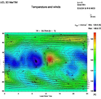
Fig. 9. The temperature and horizontal winds at the lower boundary
of the model – pressure level 1.
The MCD uses a sigma level pressure height scheme that is dependent on the surface pressure, see Eq. (6).
σ = P Ps
, (6)
where P is the pressure at a certain height, Ps is the surface
pressure and σ is the ratio of the two pressures. The sigma level system differs from the pressure level system that Mar-TIM uses, as it is dependent on the surface pressure. The differences in the pressure level schemes between MarTIM and MCD are such that a simple linear interpolation routine is used to generate a longitude-latitude dataset at a constant pressure of 0.883 Pa. This dataset contains the temperature, height, meridional and zonal winds for the new lower bound-ary of MarTIM (Moffat, 2005).
This initial interpolation is performed for MCD conditions that are low dust and with the gravity wave parameterisation deactivated. These choices were made to ensure that any dif-ferences in MarTIM output would be due only to the lower boundary and hence, the lower atmosphere. The longitude-latitude resolution of MarTIM was set to match that of the MCD input files, 5◦latitude by 5◦longitude, thus eliminat-ing the need for any further interpolations.
The MCD contains datasets that correspond to local times separated by two hours. A simple interpolation routine acts in the interface between the MCD and MarTIM and enables the creation of datasets that are separated by one hour of local time. These are then read into MarTIM at the corresponding local time. The single hour intervals in between the reading of a new dataset was decided on because a higher frequency
Fig. 10. Pressure level 30 (pressure=2.7×10⁻⁷Pa) temperature plot for MarTIM+MCD, for solar minimum, Ls=0◦.
of calls to the MCD datasets would increase the model run time by a factor of ten.
6.1 Basic MarTIM+MCD results
The effect of the MCD lower boundary on the higher pressure levels of MarTim is discussed in this section. Figure 9 shows the temperature and horizontal winds at the lower boundary of the model, pressure level 1.
This is the self-consistent input from MCD. The average temperature for this MCD lower boundary – at 152.4 K – is only half a degree cooler than have been used in the EUV+IR runs, but the variations are large – temperature up to 185.9 K and down to 129.9 K. The average height of this 0.883 Pa level is 4.3 km lower than our assumed boundary height in the rest of the runs, but the surface pressure on Mars varies by 20% due to the seasonal sublimation-condensation cy-cle, so it is difficult to be precise about pressure level al-titudes. There is obviously considerable structure in this MCD-generated boundary layer and the pressure gradients produce concomitant velocities as large as 111 ms−1, far from the uniform distribution of the EUV and IR runs, and different in structure from the tidal run.
Figure 10 gives some idea how far this structure penetrates upwards. This is the temperature at pressure level 30 to com-pare with the non-MCD case in Fig. 4.
The temperature structure has changed slightly but not sig-nificantly. There is some structure propagating up from the lower boundary, which affects the phasing of the daytime maximum: this has come forward 3–4 h. The temperature maximum has roughly the same value, but the temperature
Fig. 11. Thermospheric temperature structures at pressure level 13
(pressure=2.188×10⁻³Pa), from MCD (top) and MarTIM+MCD (bottom).
minimum has been reduced by nearly 50 K – this reflects the presence of a temperature minimum 30 K less than the average at this position in the MCD input. Figure 10 also shows the velocity vectors on this pressure level. These are not shown on Fig. 4, but the maximum and average velocities are almost the same, and the patterns are broadly similar. The only feature of note is the tendency for a second, small, tem-perature maximum near midnight, which is caused by the in-duced vertical circulation. Adiabatic contraction and advec-tion of heat induced by the circulaadvec-tion brought about by the lower boundary variability produces a heated region at the equator around 20:00–22:00 LT as low as pressure level 10, and this can then be traced up to the top – as for example in the next figure.
One advantage of the altitude overlap between MCD and MarTIM is that a comparison can be made between the two. Although they work in slightly different ways, one would expect the physics of the two models to be broadly similar and therefore, once forced to be the same at one altitude, to have broadly similar structures in the rest of the overlap volume. That this is indeed the case can be seen from Fig. 11.
Fig. 12. Comparison of meridional wind structures at pressure level
13 for MCD (top) and MCD+MarTIM (bottom).
The top panel shows the temperature structure at the 2.188×10⁻³Pa level in MCD that corresponds to pressure
level 13 in MarTIM, shown in the bottom panel. It can be seen that indeed the temperature structures are very similar even this far from the MarTIM bottom boundary (and get-ting close to MCD’s top boundary). The range of tempera-tures in MCD is larger than in MarTIM by a few 10s of % but the morphology of highs and lows is very similar. The MCD panel is overprinted with black contour lines showing how the temperature pattern ties in with the orthography of Mars, though by this altitude one might expect considerable horizontal displacement of pressure- and flow-induced fea-tures. The lower panel shows the wind velocities as well as the temperatures at this pressure level. The velocities go up to 132 ms−1, significantly up on what was seen with the
uniform lower boundary and more in line with other mod-elling results (Bougher and Dickinson, 1988), though we are unaware that significant boundary forcing was used in such models to get such lower thermosphere velocities.
Figure 12 shows, in a similar format to Fig. 11, the com-parison of the meridional velocities in MCD at the pressure
Fig. 13. The zonal wind velocity, local solar time (LST) vs. height,
from MarTIM+MCD, for solar minimum and Ls=0◦at +45◦
lati-tude.
level corresponding to pressure level 13 in MarTIM. Again the two have very similar structure, with the MarTIM ampli-tudes reduced by a few 10s of %.
6.2 Horizontal wind flow
Figures 13 and 14 can be compared to Figs. 5, 6 and Figs. 7 and 8.
Here we have the zonal and meridional winds at +45◦ lat-itude. The top level of the model shows much more variabil-ity in height than Figs. 5 and 6 because the larger temper-ature variations noted, for example, in Fig. 10, cause larger pressure variations and hence variability in the pressure level heights. Despite this apparent difference in morphology the differences in velocity are not that large. Both zonal and meridional velocities have risen in amplitude, but the max-ima and minmax-ima are no more different than about 50%. The upper thermosphere has the same structure except for an ex-tra shallow minimum around midnight in both plots. The real differences, as one would expect are lower down where there is considerably more structure in the zonal wind due to the structuring of the lower boundary. The meridional wind does not show this: however this is only one latitudinal cut through the model and so some of the structure seen at any particular pressure level (e.g. as in Figs. 11 and 12) can be missed by this sampling. It is clear there is larger variabil-ity in the lower thermosphere with MCD – however, much of this is smoothed out as one goes up to the upper
thermo-Fig. 14. The meridional wind velocity, local solar time (LST) vs height, from MarTIM+MCD, for solar minimum and Ls=0◦at
+45◦latitude.
sphere, and the averages in the lower thermosphere are not significantly different from the non-MCD runs.
The lack of significant amounts of high resolution velocity data for the thermosphere of Mars significantly hinders any consideration of how realistic these conclusions are from the model.
7 Data comparisons
7.1 Temperature
The recent missions to Mars have provided some limited data sets which can be used to validate the MarTIM results. We concentrate here on a comparison with Mars Pathfinder entry measurements. Pathfinder provided a single profile dataset containing the parameters of temperature, density and pres-sure for the following conditions: the probe entered the Mar-tian atmosphere at 03:00 local Mars time for solar minimum and Ls=143◦.
Figure 15 is the plot of Pathfinder entry temperature mea-surements compared to two MarTIM simulations under the same solar/Ls conditions – one with EUV+IR heating only and one including the (2,2) tide.
This, typically of nearly all attempts to fit detailed entry profiles (e.g. with the Viking landings), is a poor apparent fit. There is some evidence of roughly the same magnitude at 140 km and maybe above and around 100 km altitude, but the
Fig. 15. Mars pathfinder temperature profile compared to basic
MarTIM and MarTIM+(2,2) tide temperature profiles for the same conditions and position.
flight profile is extremely variable and there are sudden max-ima at 120, 80 and 60 km which the MarTIM profiles do not show. We have not done a similar comparison for MarTIM with MCD since it is obvious that, although it will have some extra variability below 140 km it still will not produce such wild behaviour. Such variable behaviour was seen by Viking as well and it is going to be a challenge to reproduce this. This variability could in part be due to the fact Pathfinder’s profile was a mix of horizontal as well as vertical travel – it moved several hundred km horizontally during this phase of its descent and there is no attempt to “map” this horizontal variability in the model output. However, it seems unlikely that even this would be able to reproduce such extremes. For-get et al. (1999) suggested that this behaviour may be due to atmospheric gravity wave (AGW) breaking in the middle Martian atmosphere. This behaviour does look similar to lidar measurements of AGWs made in the terrestrial atmo-sphere but many more measurements will be needed to say much more about this. Current work is going on to introduce a gravity wave scheme into MarTIM, but as with terrestrial GCMs this would be a global parameterisation, and would not have the small scale structure seen here. For the near fu-ture it would seem best to concentrate in GCMs on trying to get the average behaviour correct, and many more individual profiles will need to be taken to know what that average is.
7.2 Winds
It is even more difficult to validate the winds in GCMs like MarTIM. There are few direct measurements of Martian ther-mospheric winds (and even that to some extent depends on what is meant by “direct”). Mars Global Surveyor aerobreak-ing gave limited information in a restricted height and geo-graphical range – and the derived winds depend on
assump-Table 1. Northern and Southern Hemisphere data used to derive the
average zonal wind from MGS phase 2 accelerometer data, adapted from Withers (2003).
North Hemisphere South Hemisphere
Ls 30◦→50◦ 75◦→85◦
Local Solar Time 16.7 h→15.6 h 14.7 h→14.8 h Periapsis Altitude 111 km→118 km 104 km→114 km Periapsis Latitude 60◦N→30◦N 30◦S→60◦S Average Zonal Wind 74±5 ms−1 34±7 ms−1
tions that are open to question. A technique has been devel-oped to derive wind speeds from accelerometer data (With-ers, 2003), though this has not been widely used and is still under development, Table 1 shows the results obtained from MGS phase 2 accelerometer data, together with the condi-tions to which they apply.
Simulations with MarTIM to reproduce these results are difficult to set up since MGS sampled – irregularly – such a large range of conditions and geographic/LT locations. An attempt to simulate “average” MGS conditions with MarTIM with EUV and IR inputs only (no tides, no MCD) produced comparative wind speeds of 20 ms−1in the Northern Hemi-sphere and 6 ms−1in the southern. Thus, although the north-south difference was seen, the absolute values were very dif-ferent. Using the MCD-boundary version would undoubt-edly increase these values but there is some doubt about how meaningful such simulations can be made – the MGS re-sults are sampling such a range of conditions, and the tech-nique and way of averaging of the results are subject to so many questions, that to reproduce the measurement regime is unlikely to be successful. So on the velocity side it seems we must again await more, better accuracy and more easily recreated, results.
8 Conclusions
The UCL Martian thermosphere and ionosphere global cir-culation model has been developed in several stages;
– Investigating the features in the Martian thermosphere
caused by EUV/UV solar forcing
– Introducing IR heating and cooling and analysing the
effects on the thermosphere
– Introducing the (2,2) semi-diurnal tide and determining
its effects on the thermosphere
– Introducing a lower boundary that represents the lower
atmosphere from the Mars Climate Database and hence looking at some of the effects of the lower atmosphere on the Martian thermosphere
This stage-by-stage development of MarTIM has enabled the effects introduced by each new feature to be easily identi-fied and understood, e.g. the effect of introducing the semi-diurnal tide on the horizontal wind flow. It has been shown that the basic model behaves in an expected and understand-able manner. There is some concern about the magnitude of the lower atmosphere winds. The introduction of fea-tures such as the (2,2) semi-diurnal tide and the MCD lower boundary produce features that are comparable to other Mar-tian thermospheric GCMs and to the limited datasets that are available. The (2,2) semi-diurnal tide increases the horizon-tal winds in the middle atmosphere of MarTIM. However, the introduction of the MCD lower boundary that has the greatest effect on the winds in the middle atmosphere. This also had a very significant effect on the thermospheric region. Thus, inclusion of a more realistic lower boundary seems to be a precondition for reproducing the dynamics seen in the ther-mosphere.
Appendix A
Energy and momentum equation terms
Below are listed the terms used in Eqs. (1) and (2):
– V is the velocity – θ is the co-latitude – 8 is the geopotential – R is the radius of Mars
– µ is the sum of the turbulent and molecular viscosity
coefficients
– k is the unit vector in the vertical direction – ω is the vertical velocity in the pressure frame. – P is the pressure of the atmosphere
– ρ is the density of the atmosphere – is the angular velocity of Mars – g is the gravity on Mars
– H is the scale height
– ǫ is the sum of the kinetic energy plus the internal
en-ergy
– h is the geopotential height.
– KM+KT is the sum of the molecular and turbulent
con-ductivity coefficients
Acknowledgements. This work was only possible due to a Parti-cle Physics and Astronomy Research Council Ph.D studentship at University College London, UK. Thanks also go to the staff who supervised my Ph.D.
Topical Editor U.-P. Hoppe thanks S. P. Seth and another anony-mous referee for their help in evaluating this paper.
References
Angelats i Coll, M., Forget, F., Lopez-Valverde, M., Read, P., and Lewis, S.: Upper atmosphere of Mars up to 120 km: Mars Global Surveyor accelerometer data analysis with the LMD general circulation model, J. Geophys. Res., 109, e01011, doi:10.1029/2003JE002163, 2004.
Bougher, S.: Comparative terrestrial planet thermospheres, Pub-lished online, http://aoss.engin.umich.edu/people/bougher/, last accessed 2007a.
Bougher, S.: MTGCM data, Published online, http://aoss.engin. umich.edu/people/bougher/, last accessed 2007b.
Bougher, S. and Dickinson, R.: Mars mesosphere and thermosphere 1: Global mean heat budget and thermal structure, J. Geophys. Res., 93, 7325–7337, 1988.
Bougher, S. and Dickinson, R.: Mars thermosphere 2: General cir-culation with coupled dynamics and composition, J. Geophys. Res., 95, 14 811–14 827, 1990.
Bougher, S., Fesen, C., Ridley, E., and Zurek, R.: Mars meso-sphere and thermomeso-sphere coupling: Semi-diurnal tides, J. Geo-phys. Res., 98, 3281–3295, 1993.
Chapman, S. and Lindzen, R.: Atmospheric tides, D.Reidel, 1970. Forbes, J.: The upper mesosphere and lower thermosphere, vol. 87,
chap. Tidal and planetary waves, pp. 261–288, American Geo-physical Union, 1994.
Forbes, J.: Tides in the middle and upper atmospheres of Mars and Venus, Adv. Space Res., 33, 125–131, 2004.
Forget, F., Hourdin, F., Fournier, R., Hourdin, C., Talagrand, O., Collins, M., Lewis, S., Read, P., and Huot, J.: Improved general circulation models of the Martian atmosphere from the surface to above 80 km, J. Geophys. Res., 104, 24 155–24 176, 1999. Fuller-Rowell, T.: A three dimensional, time dependant global
model of the thermosphere, Ph.D. thesis, University of London, 1981.
Hanson, W., Sanatani, S., and Zuccaro, D.: The Martian ionosphere as observed by the Viking retarding potential analysers, J. Geo-phys. Res., 82, 4351–4363, 1977.
Lewis, S., Collins, M., Forget, F., and Wanherdrick, Y.: Mars Cli-mate Database v3.1 – detailed design document, Tech. rep., Uni-versity of Oxford, 2001.
Lindzen, R.: The application of terrestrial tidal theory to Venus and Mars, J. Atmos. Sci., 27, 536–549, 1970.
Lopez-Puertas, M. and Lopez-Valverde, M.: Radiative energy bal-ance of CO2non-LTE IR emissions in the Martian atmosphere, Icarus, 114, 113–129, 1995.
Lopez-Puertas, M. and Taylor, F.: Non-LTE radiative transfer in the atmosphere, World Scientific, 2001.
Lopez-Valverde, M.: Non-local thermodynamic equilibrium in gen-eral circulation models of the Martian atmosphere:1, J. Geophys. Res., 103, 16 799–16 811, 1998.
Lopez-Valverde, M. and Lopez-Puertas, M.: CO2 non-LTE cool-ing rate at 15um and its parametrisation for the Mars
atmo-sphere, Esa contract: Martian environment Models, Instituto de Astrofisica de Andalucia, Granada, Spain, 2001.
Mahajan, K. and Dwivedi, A.: Ionospheres of Venus and Mars: A comparative study, Adv. Space Res., 33, 145–151, 2004. Moffat, T.: The UCL Martian Thermosphere-Ionosphere
Model:development and validation, Ph.D. thesis, University of London, 2005.
Mueller-Wodarg, I.: Modelling perturbations through the mesopause in Earth’s upper atmosphere, Ph.D. thesis, University of London, 1997.
Mueller-Wodarg, I.: The thermosphere of Titan simulated by a global three-dimensional time-dependent model, J. Geophys. Res., 105, 20 833–20 856, 2000.
Nier, A. and McElroy, M.: Composition and structure of Mars up-per atmosphere: Results from the neutral mass spectrometers on Viking 1 and 2, J. Geophys. Res., 82, 4341–4349, 1977. Peters, B.: A Martian thermosphere/ionosphere global circulation
model, Master’s thesis, University of London, 2001.
Smith, C., Aylward, A. D., Miller, S., and Mueller-Wodarg, I.: Po-lar heating in Saturn’s thermosphere, Ann. Geophys., 23, 2465– 2477, 2005,
http://www.ann-geophys.net/23/2465/2005/.
Withers, P.: Tides in the Martian atmosphere and other topics, Ph.D. thesis, University of Arizona, 2003.