Economic valuation of energy storage coupled with photovoltaics : current technologies and future projections

(1)

Economic Valuation of Energy Storage Coupled with Photovoltaics:

Current Technologies and Future Projections

by

Trannon Mosher

B.S. Aerospace Engineering

B.A. Modern Dance

University of Colorado at Boulder, 2006

SUBMITTED TO THE DEPARTMENT OF AERONAUTICS AND ASTRONAUTICS IN

PARTIAL FULFILLMENT OF THE REQUIREMENTS FOR THE DEGREE OF

MASTER OF SCIENCE IN AERONAUTICS AND ASTRONAUTICS

AT THE

MASSACHUSETTS INSTITUTE OF TECHNOLOGY

JUNE 2010

© 2010 Massachusetts Institute of Technology. All rights reserved.

Author: _______________________________________________________________________

Department of Aeronautics and Astronautics

May 21

st

, 2010

Certified by: ___________________________________________________________________

Joshua Linn

Executive Director, MIT Future of Solar Energy

Thesis Co-Supervisor

Certified by: ___________________________________________________________________

Youssef M. Marzouk

Assistant Professor of Aeronautics and Astronautics

Thesis Co-Supervisor

Accepted by: ___________________________________________________________________

Eytan H. Modiano

Associate Professor of Aeronautics and Astronautics

Chair, Committee on Graduate Students

(2)

(3)

3

Economic Valuation of Energy Storage Coupled with Photovoltaics:

Current Technologies and Future Projections

by

Trannon Mosher

Submitted to the Department of Aeronautics and Astronautics on May 21st, 2010, in Partial Fulfillment of

the Requirements for the Degree of Master of Science

Abstract

A practical framework for the economic valuation of current energy storage systems coupled with photovoltaic (PV) systems is presented. The solar-with-storage system’s operation is optimized for two different rate schedules: (1) Time-of-use (TOU) for residential systems, and (2) Real-time wholesale rates for centralized generators. Nine storage technologies are considered for PV coupling, including six different battery chemistries, hydrogen electrolysis with a fuel cell, compressed air, and pumped-hydro energy storage. In addition, these technologies are assessed in the capacity of enabling a solar energy generator to provide a set service requirement. Concentrating solar thermal power (CSTP) with thermal storage is presented as a comparison for this final baseload scenario.

Some general insights were gained during the analysis of these technologies. It was discovered that there is a minimum power rating threshold for storage systems in a residential TOU market that is required to capture most of the benefits. This is about 1.5 kW for a 2 kWP residential PV system. It was found that roundtrip efficiency is extremely important for both TOU and real-time markets, but low self-discharge rates are even more critical in real-time rate schedules. It was also estimated that large storage systems for centralized generation would capture the most revenue with a power rating twice that of the storage capacity (2 hours of discharge). However, due to cost limitations, actual optimal ratios were calculated to be about 3 to 7 hours of discharge for operation in a real-time market.

None of the current technologies considered are able to economically meet the requirements for a residential TOU rate schedule; and only CSTP with thermal storage, pumped-hydro, and potentially compressed air storage are able to offer value in a centralized real-time market or a baseload scenario. Recommendations for future research and development (R&D) on the various storage technologies are given. For many of the electrochemical batteries, the key focus areas include cycle lifetime as well as energy and power costs. Roundtrip efficiency was identified as the weak-point of hydrogen systems; the energy cost of lithium-ion batteries was found to be prohibitively expensive for energy arbitrage applications; and the balance of system (BOS) and power costs were identified as the main focus areas for the larger pumped-hydro and compressed air storage systems.

Thesis Co-Supervisor: Joshua Linn

Title: Executive Director, MIT Future of Solar Energy Thesis Co-Supervisor: Youssef M. Marzouk

(4)

(5)

5

Acknowledgments

To my parents, for their unlimited love and support and to Cari, for being my home…

I would also like to thank my thesis advisors Josh Linn and Youssef Marzouk; whom have afforded me the flexibility to explore what interests me while offering invaluable guidance along the way. This thesis would have suffered enormously without their support.

(6)

(7)

7

List of Figures

Figure 1.1-1: U.S. Emissions by Sector with Projections to 2035 [2] ... 15

Figure 2.2-1: Potential Energy Storage Benefits Along Electricity Value Chain ... 20

Figure 2.3-1: Feasible Storage Application Ranges [19] ... 22

Figure 2.3-2: Discharge (left) and Charge (right) States of an Electrochemical Battery [20] ... 25

Figure 2.3-3: NaS Schematic [27] ... 27

Figure 2.3-4: Flow Battery Schematic [32] ... 28

Figure 2.3-5: Hydrogen Fuel Cell Schematic [19] ... 30

Figure 2.3-6: CAES Schematic [29] ... 32

Figure 2.3-7: PHES Schematic [36] ... 33

Figure 2.4-1: Insolation and Electricity Pricing Data for July 15th ... 35

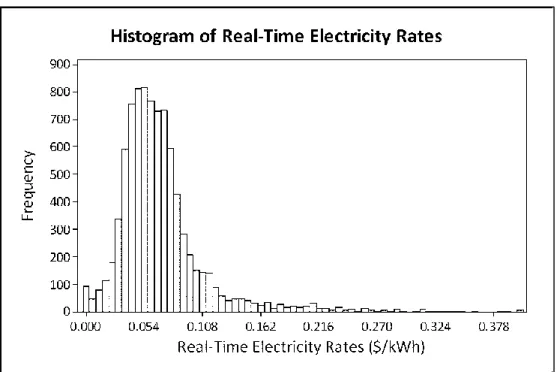
Figure 2.4-2: Real-Time Rate Schedule Histogram ... 36

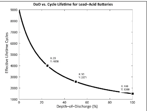
Figure 3.3-1: DoD vs. Cycle Lifetime for Lead-Acid Batteries [19]... 42

Figure 3.3-2: DoD vs. Cycle Lifetime for Lead-Acid Batteries - Extrapolation ... 43

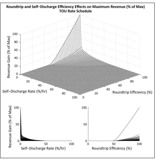
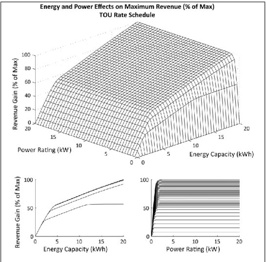
Figure 4.1-1: TOU – Efficiencies vs. Revenue Gain ... 51

Figure 4.1-2: Residential System – TOU – Ideal Storage Dispatch Profile ... 52

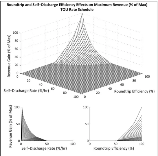
Figure 4.1-3: TOU – Efficiencies vs. Revenue Gain with Ideal Case Removed ... 53

Figure 4.1-4: TOU – Storage Size vs. Revenue Gain... 54

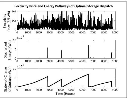
Figure 4.1-5: Residential System – TOU – Optimal Storage Dispatch Example ... 55

Figure 4.1-6: Residential System – TOU – Lead-Acid – Storage Size vs. NPV ... 56

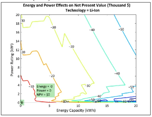
Figure 4.1-7: Residential System – TOU – Li-Ion – Storage Size vs. NPV ... 57

Figure 4.1-8: Residential System – TOU – NiCd – Storage Size vs. NPV... 58

Figure 4.1-9: Residential System – TOU – NaS – Storage Size vs. NPV ... 59

Figure 4.1-10: Residential System – TOU – VRB – Storage Size vs. NPV ... 60

Figure 4.1-11: Residential System – TOU – ZnBr – Storage Size vs. NPV ... 61

Figure 4.1-12: Residential System – TOU – H2 – Storage Size vs. NPV ... 62

Figure 4.1-13: Residential System – TOU – CAES – Storage Size vs. NPV ... 63

Figure 4.1-14: Residential System – TOU – PHES – Storage Size vs. NPV ... 64

Figure 4.2-1: Central Generation – Real-Time – Ideal Storage Dispatch Profile ... 65

Figure 4.2-2: Real-Time – Efficiencies vs. Revenue Gain with Ideal Case Removed ... 66

Figure 4.2-3: Real-Time – Storage Size vs. Revenue Gain ... 67

Figure 4.2-4: Central Generation – Real-Time – Lead-Acid – Storage Size vs. NPV... 68

Figure 4.2-5: Central Generation – Real-Time – Li-Ion – Storage Size vs. NPV ... 69

Figure 4.2-6: Central Generation – Real-Time – NiCd – Storage Size vs. NPV ... 70

Figure 4.2-7: Central Generation – Real-Time – NaS – Storage Size vs. NPV ... 71

Figure 4.2-8: Central Generation – Real-Time – VRB – Storage Size vs. NPV ... 72

Figure 4.2-9: Central Generation – Real-Time – ZnBr – Storage Size vs. NPV... 73

Figure 4.2-10: Central Generation – Real-Time – H2 – Storage Size vs. NPV... 74

Figure 4.2-11: Central Generation – Real-Time – CAES – Storage Size vs. NPV ... 75

Figure 4.2-12: Central Generation – Real-Time – PHES – Storage Size vs. NPV ... 76

Figure 4.3-1: Baseload Generation – CSTP – Thermal – Optimized Dispatch ... 77

Figure 4.3-2: Baseload Service Requirement and Dispatch Profiles... 78

(11)

11

Figure 4.3-4: Baseload Generation – PV – Lead-Acid – Optimized Dispatch ... 79

Figure 4.3-5: Baseload Generation – PV – Lead-Acid – NPV Sensitivities ... 80

Figure 4.3-6: Baseload Generation – PV – Li-Ion – Optimized Dispatch ... 81

Figure 4.3-7: Baseload Generation – PV – Li-Ion – NPV Sensitivities ... 82

Figure 4.3-8: Baseload Generation – PV – NiCd – Optimized Dispatch ... 83

Figure 4.3-9: Baseload Generation – PV – NiCd – NPV Sensitivities... 84

Figure 4.3-10: Baseload Generation – PV – NaS – Optimized Dispatch ... 85

Figure 4.3-11: Baseload Generation – PV – NaS – NPV Sensitivities ... 86

Figure 4.3-12: Baseload Generation – PV – VRB – Optimized Dispatch ... 87

Figure 4.3-13: Baseload Generation – PV – VRB – NPV Sensitivities ... 88

Figure 4.3-14: Baseload Generation – PV – ZnBr – Optimized Dispatch ... 89

Figure 4.3-15: Baseload Generation – PV – ZnBr – NPV Sensitivities ... 90

Figure 4.3-16: Baseload Generation – PV – H2 – Optimized Dispatch ... 91

Figure 4.3-17: Baseload Generation – PV – H2 – NPV Sensitivities ... 92

Figure 4.3-18: Baseload Generation – PV – CAES – Optimized Dispatch... 93

Figure 4.3-19: Baseload Generation – PV – CAES – NPV Sensitivities ... 94

Figure 4.3-20: Baseload Generation – PV – PHES – Optimized Dispatch ... 95

Figure 4.3-21: Baseload Generation – PV – PHES – NPV Sensitivities ... 96

Figure 4.3-22: Baseload Generation – PV – PHES – NPV Sensitivities with Lower Power Cost ... 97

Figure III-1: Schematic of MATLAB Code – Temporal Rate Schedules ... 117

(12)

12

List of Tables

Table 2-1: Power- and Energy-Related Capital Costs ... 23

Table 2-2: Storage Capital Cost Summary ... 24

Table 2-3: Lead-Acid Qualitative Characteristics ... 25

Table 2-4: Lead-Acid Quantitative Characteristics ... 26

Table 2-5: Li-Ion Qualitative Characteristics ... 26

Table 2-6: Li-Ion Quantitative Characteristics ... 26

Table 2-7: NiCd Qualitative Characteristics ... 27

Table 2-8: NiCd Quantitative Characteristics ... 27

Table 2-9: NaS Qualitative Characteristics ... 28

Table 2-10: NaS Quantitative Characteristics ... 28

Table 2-11: VRB Qualitative Characteristics ... 29

Table 2-12: VRB Quantitative Characteristics ... 29

Table 2-13: ZnBr Qualitative Characteristics... 29

Table 2-14: ZnBr Quantitative Characteristics ... 30

Table 2-15: H2 Qualitative Characteristics ... 30

Table 2-16: H2 Quantitative Characteristics ... 31

Table 2-17: CAES Qualitative Characteristics ... 32

Table 2-18: CAES Quantitative Characteristics... 32

Table 2-19: PHES Qualitative Characteristics ... 33

Table 2-20: PHES Quantitative Characteristics ... 33

Table 2-21: SCE TOU Rate Schedule ... 35

Table 3-1: Fixed and Control Variables - Temporal Rate Schedule Optimization ... 38

Table 3-2: Fixed and Control Variables – Baseload Generation Optimization – Step 1 ... 39

Table 3-3: Fixed and Control Variables – Baseload Generation Optimization – Step 2 ... 39

Table 3-4: Inputs and Outputs of LP Optimization ... 40

Table 3-5: Financial Inputs ... 42

Table 3-6: Inputs and Outputs of System Size LP Optimization ... 45

Table 3-7: Solar Generation Unit Costs ... 46

Table 4-1: Summary of Results with Current Technologies ... 50

(13)

13

List of Equations

Equation 2-1: Total Capital Cost for Flexible Systems ... 23

Equation 2-2: Simplified Total Capital Cost for Flexible Systems ... 24

Equation 2-3: Total Capital Cost of Fixed Systems ... 24

Equation 2-4: CAES Variable Operation Cost ... 31

Equation 2-5: Solar Energy Generation ... 34

Equation 3-1: Revenue Objective Function ... 40

Equation 3-2: Energy Generation Constraint ... 40

Equation 3-3: Energy Discharged Constraint ... 40

Equation 3-4: Capacity Limit Constraint ... 40

Equation 3-5: Power Limit Constraints ... 40

Equation 3-6: Effective Cycle Lifetime ... 43

Equation 3-7: Number of Required Capital Purchases ... 43

Equation 3-8: Scaled PCS Cost... 44

Equation 3-9: O&M Cost ... 44

Equation 3-10: NPV Calculation ... 44

Equation 3-11: Annual Cashflow Relationship ... 45

Equation 3-12: PV Service Requirement Constraint ... 46

Equation 3-13: CSTP Service Requirement Constraint ... 46

Equation 3-14: PV System Size Optimization Objective Function ... 46

(14)

14

List of Acronyms

AC Alternating Current

AM1.5G Air Mass 1.5 Global constant BOS Balance of System

CAES Compressed Air Energy Storage CAISO California Independent System

Operator

CO2 Carbon Dioxide

CSTP Concentrating Solar Thermal Power

DC Direct Current

DNLP Discrete Non-Linear Program DoD Depth-of-Discharge

DOE Department of Energy EERE Energy Efficiency and

Renewable Energy laboratory EIA Energy Information

Administration

GAMS General Algebraic Modeling System

GHG Green House Gases

H2 Hydrogen

Insolation Incident Solar Radiation IPCC Intergovernmental Panel on

Climate Change kW/MW Kilowatt/Megawatt

kWh/MWh Kilowatt-hour/Megawatt-hour

Li-ion Lithium-ion

LP Linear Program

NaS Sodium Sulfur

NCDC National Climatic Data Center NiCd Nickel Cadmium

NLP Non-Linear Program NOAA National Oceanic and

Atmospheric Administration NPV Net Present Value

NSRDB National Solar Radiation Database

O&M Operation and Maintenance PCS Power Control System

PHES Pumped-Hydro Energy Storage

PQ Power Quality

PV Photovoltaic

R&D Research and Development SCE Southern California Edison SETP Solar Energy Technologies

Program

SNL Sandia National Laboratories T&D Transmission and Distribution

TOD Time-Of-Day

TOU Time-Of-Use

VRB Vanadium Redox Battery ZnBr Zinc-Bromide

(15)

1. Introduction

The Earth’s climate is changing, with the global temperature now poised to rise more than a degree from its historical average, marking the largest deviation in over 10,000 years [1]. It has become apparent that the human processes of green house gas (GHG) emission and deforestation are the largest contributing factors to this unparalleled trend. With GHG emissions already exceeding the worst-case scenario projected by the Intergovernmental Panel on Climate Change (IPCC) [1], immediate action is not only required to mitigate future detrimental effects on human society, it is a moral obligation to the global ecosystem we are a part of. This is the underlying motivating factor for this work.

The following figure is compiled from CO2 emissions projections by the Energy Information Administration (EIA) [2]; with the residential, commercial, and industrial sectors shown excluding electricity use. It can be seen that the electric power sector is responsible for approximately 40% of all U.S. CO2 emissions and this does not look likely to change in the near future.

Figure 1.1-1: U.S. Emissions by Sector with Projections to 2035 [2]

Renewable energy technologies are a beacon of hope in this grim situation. However, there are major hurdles to the widespread adoption of many of these technologies to meet the nation’s electricity needs; notably, intermittency and cost. The intermittent nature of renewable energy generation arises when the fuel source cannot be controlled directly. For example, solar can only produce energy when the sun is up, and wind turbines can only operate when it is windy. Although this work looks at photovoltaic (PV) solar generation, the principles and methods could be readily expanded to wind, tidal/ocean, or other intermittent generation sources. PV was chosen because it is one of the most

0% 20% 40% 60% 80% 100% 2007 2009 2011 2013 2015 2017 2019 2021 2023 2025 2027 2029 2031 2033 2035

U.S. CO2 Emissions by Sector

Electric Power Transportation Industrial Commercial Residential

(16)

16

rapidly growing renewable energy markets in the world. From an increasing penetration perspective, it becomes prudent to assess various means of controlling the intermittency, while at the same time increasing the value of this energy service. Relevant markets and scales include residential and centralized generation. On a longer time-scale, PV may be asked to provide a set service requirement as renewable energy technologies are required to provide baseload generation. This thesis will look at all three scenarios in turn.

The use of energy storage has the potential to help with both controlling intermittency as well as adding value to the system. In a time-varying electricity market (i.e. time-of-use or real-time pricing), storage can be used to shift generation from periods of low prices (off-peak) to those of higher worth (peak), as recognized by the Department of Energy’s (DOE) Energy Efficiency and Renewable Energy (EERE) in the Solar Energy Technologies Program (SETP) Plan:

Energy storage is an important element of advanced power management systems, as adding storage to a PV system has the potential to increase its value. [3]

Although this benefit may be the economic driving force behind the development and implementation of energy storage, it may also enable significant quantities of renewable generation on the electric grid, as the Power Quality Systems Director for the Power Quality Products Division of S&C Electric Company, Brad Roberts, noted:

The real benefit [of storage] will come from optimizing the value of wind and solar resources by capturing even more megawatt hours of clean energy to power the world’s ever expanding electric grids. [4]

There are several methods for handling the undesirable affects of intermittency (such as demand-side response and/or coupling solar with other generators). This work considers the use of energy storage to control the dispatch of centralized solar generation under the constraint of meeting a specific service requirement.

1.1. Central Questions

Utilizing energy storage with renewable generation, as well as to facilitate electricity grid functions, has been prevalent in recent literature (the reader is referred to many of the works cited in this thesis). Most of this work, however, looks at the benefit gained (economic and environmental) by adding the

concept of energy storage, independent of current cost and/or performance metrics. For example,

(17)

17

costs or performance of a specific storage technology [5]. Their goal is to develop an algorithm to optimize the dispatch of energy storage with wind generation, given both are already available. Another common approach is to explore a purely mathematical framework for the optimization of an unspecified generator with a black-box storage device; like in the work of Bannister and Kaye where they look at a novel method for the rapid optimization of storage systems [6]. Beyond pumped-hydro [7],[8] – see section 2.3.10 for technology description – the author has found little if any analysis assessing the state of current storage technologies in the context of being able to fully capture these benefits. Many of the benefits reported in these studies are not fully realizable with current technologies, or they are limited to niche markets. Valuable insight may be gained by looking at the economic and technological benchmarks that future storage technologies must meet in order to make these benefits accessible to larger markets. The central questions of this work thus become:

1. What is the current state of energy storage technologies in being able to capture benefits from a residential TOU electricity rate schedule?

2. What is the current state of energy storage technologies in being able to capture benefits from a wholesale real-time electricity rate schedule?

3. What is the current state of energy storage technologies in enabling centralized generation to meet a specified service requirement?

4. What are the future technological and economic benchmarks for storage to more fully capture these benefits?

In this work, ‘larger markets’ are taken to be grid-connected residential PV systems as well as centralized photovoltaic (PV) generation (utility-scale plants) in temporal electricity rate structures. It has also been common practice in recent work to optimize the charge/discharge profile of a storage device for only one day in advance. This is rational in a real-time market because the electricity price forecast accuracy degrades considerably the further into the future it is projected; hence, optimizing a storage profile for a week in advance would not make much sense. However, for residential time-of-use (TOU) rate schedules, the price forecast is known precisely. With this in mind, an optimization method is employed that allows for nocturnal, weekly, or seasonal energy arbitrage (time-shift of energy) to assess any additional utility that may be gained over the traditional daily optimization method for the appropriate markets. However, it is speculated that the added cost and energy losses due to physical limitations of the various storage devices will limit the optimization timeframe to within the realm of real-time pricing forecast error limitations.

(18)

18

This work aims to contribute both a novel means for optimizing energy storage investments as well as offering a snapshot of current storage technologies in the context of being able to enter the energy arbitrage market on a residential as well as a centralized scale. Further insights are offered as to what future energy storage technologies might look like in order to reap these benefits more fully.

(19)

19

2. Background

2.1. Review of Solar Energy

Incident solar radiation (insolation) can be harvested and transformed into a usable energy form by three different processes: thermal capture, the photovoltaic effect, or direct fuel production. The first method has been around since the 7th_{century B.C., when glass and mirrors were used to concentrate} the sun’s rays to start fires; and it was incorporated into passive solar building design as early as the 1st century A.D. [9]. The photovoltaic effect was discovered in 1839 by French scientist Edmond Becquerel [9], but it wasn’t until the 1950s that modern crystalline silicon PV cells were discovered and then developed primarily for a very specific niche market: the space race [10]. Generating fuels from sunlight, like splitting water to yield hydrogen via artificial photosynthesis, has been the most recent development in capturing the sun’s power. The recent work by MIT Professor Daniel Nocera has been very promising in this area [11].

This thesis will focus on the use of energy storage with photovoltaic (PV) generation. The other two solar technologies do not lend themselves to this analysis as readily because (1) solar fuel technologies generate their own storage by the very definition of their process (hence the reason for much of their appeal), and (2) solar thermal technologies have already been relatively successfully integrated with thermal storage. Recent work has been done with integrating a thermal storage medium (usually molten salt) into concentrating solar thermal power (CSTP) systems, both via government demonstration projects [12], as well as promising new research to increase efficiency and decrease cost of this technology [13],[3]. A natural advantage of developing storage for CSTP is the fact that no energy conversion is required for thermal storage. CSTP with thermal storage is used as a comparison for the baseload scenarios looked at in the last sections of this thesis. For PV, however, the energy being generated is in direct current (DC), which cannot be stored directly. Current electric energy storage technologies convert this electricity into another medium that can be stored such as heat (thermal storage), kinetic energy (mechanical storage), electrochemical energy (chemical batteries), or chemical bonds (fuels). The various technologies relevant to this work that exploit these processes are discussed in Section 2.3.

(20)

20

2.2. Review of Energy Storage Markets

There are many different potential markets available for energy storage, both for interfacing with a generation source as well as being used directly on the grid. Energy storage applications can be divided into two general functions: (1) power quality (PQ), and (2) energy arbitrage. This work will focus on the latter, primarily because the PQ market is already showing signs of being exploited [14]. Before the energy storage functions are broken down, definitions of common energy market terms are given.

Power Quality – Can include frequency and voltage regulation as well as backup power in case of

outages.

Energy Arbitrage – Involves the storage of energy when the price and/or demand (usually both) is low,

and then discharging/selling the energy when the price and/or demand is high.

Load-Following – Is the use of a storage device to match the generation profile of the grid to the rapidly

fluctuating demand profile on the end-user side.

Frequency Regulation – Is the use of energy storage to maintain the frequency within the tolerance

limits of the generators. The frequency can drop under conditions when demand increases faster than new generation can come online.

Transmission and Distribution (T&D) Deferral – Involves the temporary use of a storage device to allow

the existing transmission line to operate for a longer time without being upgraded or replaced by increasing the peak-capacity of the transmission line.

TOU Cost Reduction – Is energy arbitrage on the user side of the meter to shift consumption from

periods of high electricity rates to those of lower cost (end-user energy arbitrage).

Energy storage functions can be beneficial when supplied along a variety of locations on the electricity value chain [15].

Figure 2.2-1: Potential Energy Storage Benefits Along Electricity Value Chain

The basic functions shown in Figure 2.2-1 are: supplementing existing generation sources (power quality and/or energy arbitrage), deferring upgrades of generators or transmission and distribution (T&D) lines, avoiding congestion in the transmission stage, load following (can be in the generation, distribution, or consumption functions), and several end-user benefits [15]. Everything prior to end-user

Generation

•Supplement current generators •Defer upgrades

Transmission

•Defer upgrades •Avoid congestion •Frequency regulation

Distribution

•Defer upgrades •Load following •Power quality

Consumption

•TOU cost reduction •Demand charge reduction •Power quality

(21)

21

consumption can be viewed as “utility-scale” or “centralized” applications, whereas the consumption section of the value chain is referred to as “residential-“ or “commercial-scale”.

In addition to the economic benefits along the value chain, environmental benefits may be realized from the use of energy storage. It is possible to arbitrage energy such that energy from cleaner generators (natural gas) offset the emissions from dirtier sources (coal and oil). However, it has been shown that significant revenue losses can be observed if a storage system is optimized purely for environmental benefit within a real-time pricing market [16]. Of course, if a price on GHG emissions were imposed, optimizing for economic benefits would at least partially include environmental concerns as well. Therefore, it is simplest to think of the optimization procedure as being with respect to perceived economic benefit, which may or may not reflect environmental effects.

Unfortunately, there are significant regulatory barriers that prevent storage technologies from capturing revenue streams from many of these markets. Notably, all of the T&D functions and many of the generation functions do not have a regulatory framework to facilitate integration into their rate base. A recent report by Pike Research LLC stated this problem concisely:

Major regulatory hurdles must be met before storage can even be considered for use in some markets. According to the newly established Electricity Advisory Council, no cohesive plan exists as to how storage technologies will be incorporated into the grid. In addition, the current system does not credit the value of storage across the entire utility value chain. Generation, transmission and distribution are typically viewed discretely. The resulting challenge is the complete lack of a cost recovery system, and with no clear path for cost reimbursement, most utilities have opted not to invest in energy storage. It is easier for utilities to make investments in conventional approaches to addressing grid instability, such as natural gas spinning reserves, as these investments are sure to be covered by the regulatory rate base. [17]

Another issue that the above excerpt refers to is the fact that a single energy storage device is currently unable to capture revenues from multiple services along the value chain. A report by the DOE’s Sandia National Laboratories (SNL) summarizes additional benefits of utilizing storage with renewable generation that are not accounted for in the current regulatory framework:

Depending on where the storage is located, if it is used in conjunction with bulk renewables resources, then the benefits may also include: 1) avoided/deferred need to build or to purchase other generation capacity, 2) avoided/deferred need to build transmission capacity, 3) avoided transmission access charges, 4) avoided transmission congestion charges, 5) transmission support, and 6) ancillary services. [18]

As mentioned at the beginning of this section, this work focuses on the energy arbitrage market. The primary reason being that the PQ market has key players (ex. Beacon Power Corporation [14]) who have already entered onto the scene; whereas the only major players in the energy arbitrage market are

(22)

22

geographically limited (pumped-hydro and compressed air energy storage). Energy arbitrage also offers the unique possibility of enabling baseload/firm generation from intermittent renewable energy sources, which is looked at in Section 4.3.

2.3. Review of Current Energy Storage Technologies

Within the framework of energy arbitrage, as discussed in the previous section, current energy storage technologies are evaluated on their potential to serve this market. The grayed-out region of Figure 2.3-1 indicates several storage technologies that are not appropriate for arbitrage. These include superconducting magnetic energy storage (SMES) systems, flywheels (low- and high-speed), and supercapacitors. The remaining storage technologies that could potentially perform arbitrage services are electrochemical batteries, flow batteries, compressed air energy storage (CAES), and pumped-hydro energy storage (PHES). Another technology which is not listed in the figure, but which is considered in this work, is electrolysis with hydrogen storage and a fuel cell (H2). Each technology considered in the analysis is described briefly in the following sections. First, however, an explanation of the dynamics of energy storage capital cost is given.

(23)

23

2.3.1. A Note on Storage Capital Cost Estimation

While compiling cost information for this work, it was discovered that estimating the capital cost of a large storage facility can be an area of significant confusion, and is rarely addressed clearly (or even explicitly) in the literature. Hence, some clarifications are made here before the storage technologies are described.

Table 2-1: Power- and Energy-Related Capital Costs

Capital Expenditures Power-Related BOS Cost ($/kW)

Energy-Related BOS Cost ($/kWh) Power-Related Storage Cost ($/kW) Energy-Related Storage Cost ($/kWh)

The balance-of-system (BOS) cost is usually given as per unit power ( ) or per unit energy ( ), whereas the unit cost of actual storage device is given both on a power ( ) and an energy ( ) basis, as shown in Table 2-1. In addition, the BOS expense is often included in the unit storage costs. The cost of the power control system (PCS) is often included in the capital cost estimate; however, it is kept separate here because of the difference in the PCS lifetime and the total solar-with-storage system lifetime (see Section 3.3.2 for how PCS cost is included). An important distinction in storage system architectures must be addressed here. If a storage device is able to be sized for power and energy independently of one another, then the unit power and energy costs are given as separate components from which the total cost must be obtained by summing over power and energy requirements. If, however, the storage cell has a fixed power/energy ratio, then the costs are given as a complete system cost and either the power or the energy component must be used to find the total capital cost (whichever is higher). For example, if a 1 kW / 1 kWh battery cell cost $100 and the power and energy components cannot be sized independently, then the unit capital cost of this device would be either $100/kW or $100/kWh, and even if the storage requirement were only 1 kW / 0.5 kWh, the battery would still cost $100. The former system architecture will be referred to as a “flexible” system, and the latter as a “fixed” system for convenience.

For flexible systems, the capital cost may be computed as:

Equation 2-1: Total Capital Cost for Flexible Systems

In this expression, is the balance of system cost per unit power ($/kW), is the balance of system cost per unit energy ($/kWh), is the storage cost per unit power ($/kW), is the storage cost

(24)

24

per unit energy ($/kWh), is the power rating of the storage device (kW), and is the energy capacity of the storage device (kWh). This expression can be re-written as:

Equation 2-2: Simplified Total Capital Cost for Flexible Systems

if the total unit power cost is defined as , and the total unit energy cost is defined as .

For the fixed systems, the capital cost must be calculated as:

Equation 2-3: Total Capital Cost of Fixed Systems

In this expression, is the maximum of the power and energy costs, respectively. Note that this expression does not lend itself to the simplification shown in Equation 2-2. A summary of these power- and energy-related costs for each technology to be analyzed is shown in Table 2-2 below.

Table 2-2: Storage Capital Cost Summary

Storage Technology Lead-Acid Li-Ion NiCd NaS VRB ZnBr H2 CAES PHES System Architecture Fix Fix Fix Fix Flex Flex Flex Flex Flex Power-Related ($/kW) $0 $0 $0 $20 $0 $0 $0 $0 $0 $250 $333 $6,020 $1,500 $700 $300 $500 $425 $600 Energy-Related ($/kWh) $50 $0 $92 $0 $0 $0 $0 $50 $0 $150 $1,333 $600 $176 $230 $250 $15 $2 $12

The entries with a zero cost have already included this expense in the or metrics.

Taking a large, 10 MW / 85 MWh, Sodium Sulfur (NaS) battery plant as an example, the distinction between the two system architectures can be illustrated. Using the proper method, where the energy and power components of the battery cell itself are fixed and cannot be sized independently, as shown in Equation 2-3, the upfront capital cost of the system would be:

However, if we assume energy and power are sized independently with the same respective unit costs for each as shown in Equation 2-1, then the capital cost would be nearly twice as much:

(25)

25

Note that these capital costs do not include the PCS or fixed operation and maintenance (O&M) costs, which are discussed in Section 3.3.2.

2.3.2. Lead-Acid Batteries

A schematic of the discharge and charge states of an electrochemical battery (not just lead-acid) is shown in Figure 2.3-2 below. For a acid battery, the oldest rechargeable battery chemistry, lead-dioxide serves as the cathode electrode, lead as the anode, and sulfuric acid is used as the electrolyte [20].

Figure 2.3-2: Discharge (left) and Charge (right) States of an Electrochemical Battery [20]

The main advantages of lead-acid batteries are their low capital and operation costs, and high efficiencies. However, their limited cycle and calendar lifetimes make them much less economical in energy arbitrage applications. These qualitative characteristics are summarized in Table 2-3.

Table 2-3: Lead-Acid Qualitative Characteristics

Advantages Disadvantages Low Capital Cost Low Cycle Lifetime Good Roundtrip Efficiency Low Calendar Lifetime Low Self-Discharge

When available, key cost and performance metrics were obtained from the Sandia National Laboratories (SNL) 2001 report on energy storage characteristics and technologies (reference [21]). However, many other sources were utilized in an attempt to obtain the most recent information, and for technologies not listed in the SNL report. The key parameters for lead-acid batteries are listed in Table 2-4.

(26)

26

Table 2-4: Lead-Acid Quantitative Characteristics

Parameter Value

Energy-Related Cost $150/kWh [22] Power-Related Cost $250/kW [21] Balance of System Cost $50/kWh [21] Fixed O&M Cost $1.55/kW-yr [21] Variable O&M Cost $0.01/kWh [21] Roundtrip Efficiency 87.5% [21],[20] Self-Discharge Rate 2%/month [20] Cycle Lifetime ~1,500 [20] Calendar Lifetime 10 years [20]

2.3.3. Lithium-Ion (Li-Ion) Batteries

Li-ion batteries have the same basic electrochemical architecture shown in Figure 2.3-2 above. In this case, the cathode is comprised of a lithiated metal oxide (such as LiCoO2 or LiMO2), the anode is made of graphitic carbon, and the electrolyte is composed of a lithium salt [23]. Li-ion batteries tend to be most beneficial for portable frequency regulation type applications because of their excellent energy density and much higher cycle lifetimes at lower depths-of-discharge (>3,000 at 80% DoD [23]).

Table 2-5: Li-Ion Qualitative Characteristics

Advantages Disadvantages Excellent Efficiencies High Cost

High Energy Density Low Cycle Lifetime

A summary of the qualitative characteristics is shown above in Table 2-5, and the quantitative metrics are given in Table 2-6.

Table 2-6: Li-Ion Quantitative Characteristics

Parameter Value

Energy-Related Cost $1,333/kWh [24],[22] Power-Related Cost $333/kW [24] Balance of System Cost Included Fixed O&M Cost N/A [25] Variable O&M Cost N/A [25] Roundtrip Efficiency ~95% [20]

Self-Discharge Rate ~3%/month [20],[25] Cycle Lifetime 1,500 [20]

Calendar Lifetime 15 years [26]

2.3.4. Nickel-Cadmium (NiCd) Batteries

As with lead-acid and Li-ion batteries, the electrochemical architecture for NiCd batteries is the same as shown in Figure 2.3-2 above. The NiCd chemistry has been around almost as long as lead-acid batteries. They use nickel hydroxide for the anode material, cadmium hydroxide as the cathode, and an aqueous solution of mostly potassium hydroxide (small amounts of lithium hydroxide) as the electrolyte [25].

(27)

27

Table 2-7: NiCd Qualitative Characteristics

Advantages Disadvantages Long Calendar Lifetime Higher Cost

Reliability Moderate Efficiencies

A summary of the qualitative characteristics is shown above in Table 2-7, and the quantitative metrics are given in Table 2-8.

Table 2-8: NiCd Quantitative Characteristics

Parameter Value

Energy-Related Cost $600/kWh [22] Power-Related Cost $6,020/kW [25] Balance of System Cost $92/kWh [25] Fixed O&M Cost $97/kW-yr [25] Variable O&M Cost $0 [25]

Roundtrip Efficiency 74% [20] Self-Discharge Rate 10%/month [20] Cycle Lifetime ~2,250 [20] Calendar Lifetime 17 years [20]

2.3.5. Sodium-Sulfur (NaS) Batteries

Whereas most electrochemical batteries contain solid anodes and cathodes, and a liquid electrolyte; NaS batteries are comprised of liquid sulfur as the anode, liquid sodium as the cathode, and are separated (the “electrolyte”) by a solid alumina ceramic [27]. This system architecture is shown in Figure 2.3-3. To maintain proper functioning, the liquid sulfur and sodium are kept at about 3000C. This parasitic heat requirement is responsible for the relatively high self-discharge of ~17% per day [28].

(28)

28

The qualitative and quantitative characteristics are given in Table 2-9 and Table 2-10, respectively.

Table 2-9: NaS Qualitative Characteristics

Advantages Disadvantages

Good Cycle & Calendar Lifetime Fairly Expensive

Parasitic Energy Requirement

Table 2-10: NaS Quantitative Characteristics

Parameter Value

Energy-Related Cost $176/kWh [29] Power-Related Cost $1,500/kW [29] Balance of System Cost $20/kW [29] Fixed O&M Cost $9/kW-yr [30] Variable O&M Cost $0 [30] Roundtrip Efficiency 76% [30],[31] Self-Discharge Rate ~17%/day [28] Cycle Lifetime >3,000 [30] Calendar Lifetime 15 years [30]

2.3.6. Vanadium Redox Flow Batteries (VRB)

A schematic of how a flow battery operates is shown in Figure 2.3-4. A liquid electrolyte is stored in external tanks and is pumped into reaction stacks (fuel cells) that converts the chemical energy into electricity (during discharge) or electricity into chemical energy (during charge) [29]. An advantage of flow batteries over conventional batteries is that the energy capacity (as determined by the volume of electrolyte and size of the storage tanks) can be sized independently from the power rating (as determined by the size of the reaction stacks).

(29)

29

Another advantage is that although the reaction stacks of VRBs require replacement every 1,000 cycles or so, this is only a fraction of the entire system cost (~$375/kW) and most of the system will continue to operate for the lifetime of a PV array [29]. Refer to Table 2-11 for a summary of the qualitative characteristics, and Table 2-12 for the quantitative metrics.

Table 2-11: VRB Qualitative Characteristics

Advantages Disadvantages

Energy and Power Sized Independently Mechanical Complexity

Good Efficiencies Moderate Parasitic Losses (due to pumps) Long Lifetime of Electrolyte/Tanks

Table 2-12: VRB Quantitative Characteristics

Parameter Value

Energy-Related Cost $230/kWh [29] Power-Related Cost $700/kW [29] Balance of System Cost Included Fixed O&M Cost $4/kW-yr [29] Variable O&M Cost $0 [29] Roundtrip Efficiency 85% [29],[33] Self-Discharge Rate 7.5%/month [31] Cycle Lifetime 1,250 [29] Calendar Lifetime 12 years [29]

2.3.7. Zinc-Bromide (ZnBr) Flow Batteries

The operational characteristics of a ZnBr flow battery is the same as shown in Figure 2.3-4. Although the efficiencies are slightly below that of VRB, ZnBr flow batteries have a lower cost and at least one major manufacturing company (Premium Power, located in North Reading, MA) claims unlimited deep cycling capability. The company is very secretive about their metrics, however, and no justifications are given for this claim [24],[34]. Since a source could not be found that states otherwise, Premium Power’s numbers were assumed accurate for the purposes of this analysis. A summary of the qualitative and quantitative metrics are given in Table 2-13 and Table 2-14, respectively.

Table 2-13: ZnBr Qualitative Characteristics

Advantages Disadvantages Low Cost Moderate Efficiencies Excellent Lifetime

(30)

30

Table 2-14: ZnBr Quantitative Characteristics

Parameter Value

Energy-Related Cost $250/kWh [24] Power-Related Cost $300/kW [24] Balance of System Cost Included Fixed O&M Cost N/A [21]

Variable O&M Cost $0.004/kWh [34] Roundtrip Efficiency 75% [35]

Self-Discharge Rate 13.5%/month [31] Cycle Lifetime Lifetime [34] Calendar Lifetime 30 years [34]

2.3.8. Hydrogen Electrolysis with Fuel Cell (H2)

There are three key processes of a hydrogen storage system: electrolysis which uses electricity to produce hydrogen from water, storage of the hydrogen (many different forms/states can be used), and the use of a fuel cell to generate electricity from the stored hydrogen when it is desired. A schematic of how the fuel cell functions is shown in Figure 2.3-5. As with flow batteries, the energy and power ratings can be sized independently for a H2 system. However, the roundtrip efficiency is considerably less than flow batteries.

Figure 2.3-5: Hydrogen Fuel Cell Schematic [19]

A summary of the qualitative and quantitative metrics are given in Table 2-15 and Table 2-16, respectively.

Table 2-15: H2 Qualitative Characteristics

Advantages Disadvantages Low Energy Cost Low Efficiencies Good Lifetime O&M Cost

(31)

31

Table 2-16: H2 Quantitative Characteristics

Parameter Value

Energy-Related Cost $15/kWh [21] Power-Related Cost $500/kW [21] Balance of System Cost Included [21] Fixed O&M Cost $10/kW-yr [21] Variable O&M Cost $0.01/kWh [21] Roundtrip Efficiency 59% [21] Self-Discharge Rate 3%/day [20] Cycle Lifetime Lifetime [21] Calendar Lifetime 17 years [21],[25]

2.3.9. Compressed Air Energy Storage (CAES)

CAES technology has been commercially developed since the late 1970s, but there is only one CAES facility in the U.S., which has been operating since 1991 in McIntosh, Alabama [29]. This is the only storage technology considered which has a fuel cost associated with its operation. In a CAES system, electricity is used to compress air during the charge cycle which is then released, heated in an expansion chamber with natural gas, and used to drive combustion AC turbines during the discharge cycle (see Figure 2.3-6).

The variable cost associated with the use of natural gas during the discharge cycle can be computed from the following relationship:

Equation 2-4: CAES Variable Operation Cost

Assuming a fuel cost of $3/MMBtu and a heat rate of 4,000 Btu/kWh [29], this equates to a variable O&M of $0.012/kWh. An interesting characteristic of CAES plants is that 2-3 times more energy is released during the discharge cycle than is spent in the compression stage. This is because of the additional energy from the natural gas. A simplification is made in this work by using an “effective” roundtrip efficiency of 85%, which accounts for the use of the fuel in the operational cycle [29].

(32)

32

Figure 2.3-6: CAES Schematic [29]

For large CAES plants, it is most economical to store the compressed air in large underground caverns (salt caverns, rock caverns, or porous rock formations) [29]. The costs/metrics listed in this work correspond to CAES in salt caverns. Although somewhat geographically limited, CAES may still be viable for over 80% of the United States [29]. The qualitative and quantitative characteristics of this technology are shown in Table 2-17 and Table 2-18, respectively.

Table 2-17: CAES Qualitative Characteristics

Advantages Disadvantages Low Cost Geographically Limited Good Efficiencies

Excellent Lifetime

Table 2-18: CAES Quantitative Characteristics

Parameter Value

Energy-Related Cost $2/kWh [29],[21] Power-Related Cost $400/kW [29],[21] Balance of System Cost $50/kWh [21] Fixed O&M Cost $1.42/kW-yr [21] Variable O&M Cost $0.012/kWh [29] Roundtrip Efficiency 85% [29] Self-Discharge Rate 0% [21] Cycle Lifetime Lifetime [21] Calendar Lifetime 30 years [21]

2.3.10. Pumped-Hydro Energy Storage (PHES)

In PHES, the potential energy contained in an elevated body of water serves as the energy capacity. Generation and pumping can either be accomplished by single-unit reversible pump-turbines, or by separate pumps and generators [21]. Water is pumped from a lower reservoir up to the elevated

(33)

33

reservoir during the charge cycle, and is released back down to the lower reservoir during discharge (see Figure 2.3-7).

Figure 2.3-7: PHES Schematic [36]

This technology has been in development since the 1920s [21]. The qualitative characteristics are the same as for CAES and are shown in Table 2-19. The quantitative metrics are given in Table 2-20.

Table 2-19: PHES Qualitative Characteristics

Advantages Disadvantages Low Cost Geographically Limited Good Efficiencies

Excellent Lifetime

Table 2-20: PHES Quantitative Characteristics

Parameter Value

Energy-Related Cost $12/kWh [21] Power-Related Cost $600/kW [21] Balance of System Cost Included Fixed O&M Cost $3.8/kW-yr [21] Variable O&M Cost $0.0038/kWh [21] Roundtrip Efficiency 87% [21]

Self-Discharge Rate 0% [21] Cycle Lifetime Lifetime [21] Calendar Lifetime 30 years [21]

2.4. Description of Case Studies

In order to assess the value of adding energy storage in arbitrage applications, three case studies were chosen within the context of “larger markets”. All three case studies are located close to Blythe, California, so that the level of incident solar radiation (insolation) would be consistent throughout. Blythe is also desirable because a local utility company, Southern California Edison (SCE), offers a TOU

(34)

34

rate schedule. For the real-time pricing rates an average across the California Independent System Operator’s (CAISO) entire region was used. The following subsections describe the relevant regional datasets.

2.4.1. Insolation Data

The insolation data for Blythe, CA, were obtained from the National Solar Radiation Database (NSRDB) as provided by the National Climatic Data Center (NCDC). Richard Perez, at the State University of New York in Albany, resolved high-resolution satellite data (10 km grid-squares) into both global and direct insolation components. Global insolation data are used for the PV simulations because the photovoltaic effect occurs with both direct and diffuse solar radiation, and the direct insolation data are used for the baseload concentrating solar thermal power (CSTP) simulations. This insolation data can be publicly downloaded from the National Oceanic and Atmospheric Administration’s (NOAA) website cited here: [37]. In an attempt to simulate the average value of adding storage to a PV system, data from 1997 – 2005 were averaged to obtain a typical year. This insolation dataset, along with the electricity rates described below, is plotted for July 15th in Figure 2.4-1.

Hourly generation was computed from this hourly insolation data by multiplying the insolation for a given hour ( in Wh/m2) by the peak watt rating of the system ( ), and dividing by 1,000 W/m2, the global Air Mass ( ) constant [38]:

Equation 2-5: Solar Energy Generation

2.4.2. Pricing Data

The real-time hourly location marginal pricing (LMP) data were obtained from the CAISO public download site listed in the bibliography under this citation: [39]. The pricing dataset for 2008 was used, as this was the most recent complete dataset at the time it was retrieved. Since 2008 was a leap-year, pricing data for February 29th were removed from the dataset so that the timestamp would match the hourly insolation data (which omitted data from the leap-years of 2000 and 2004 before averaging). As seen in Figure 2.4-2, the bulk of wholesale electricity prices are in the range of 1 – 10 ¢/kWh with only a handful of peak-prices on the order of 25 – 40 ¢/kWh. Therefore, the value of energy arbitrage lies within shifting as much generation as possible from the bulk hours to the relatively few peak-price hours. The TOU rate schedule for SCE has both a time-of-day (TOD) and a seasonal variation. These distinctions are shown in Table 2-21. This rate schedule was obtained from the SCE utility company.

(35)

35

Table 2-21: SCE TOU Rate Schedule

Season / TOD Electricity Price Winter Off-Peak 17.59 ¢/kWh Winter Peak 21.24 ¢/kWh Summer Off-Peak 18.44 ¢/kWh Summer Peak 36.06 ¢/kWh

Figure 2.4-1: Insolation and Electricity Pricing Data for July 15th

$0.00 $0.05 $0.10 $0.15 $0.20 $0.25 $0.30 $0.35 $0.40 0 200 400 600 800 1000 1200 1 2: 0 0 A M 1 :0 0 A M 2 :0 0 A M 3 :0 0 A M 4 :0 0 A M 5 :0 0 A M 6 :0 0 A M 7 :0 0 A M 8 :0 0 A M 9 :0 0 A M 1 0: 0 0 A M 1 1: 0 0 A M 1 2 :0 0 P M 1 :0 0 P M 2 :0 0 P M 3 :0 0 P M 4 :0 0 P M 5 :0 0 P M 6 :0 0 P M 7 :0 0 P M 8 :0 0 P M 9 :0 0 P M 1 0 :0 0 P M 1 1 :0 0 P M El ec tr ic ity P ri ce ( $/ kW h ) In so la ti o n (W h /m 2) Time of Day

Insolation and Rate Schedules for July 15

th

(36)

36

Figure 2.4-2: Real-Time Rate Schedule Histogram

2.4.3. Load Data

For the last case-study, solar-with-storage systems were evaluated within a baseload generation role. This was simulated by requiring the generator to meet a specific demand profile. The demand profile was calculated by scaling CAISO’s hourly load by a base system size (10 MW). The hourly system load data were obtained from CAISO’s public download site mentioned previously, and can be accessed under this reference: [39].

(37)

37

3. Modeling Methodology

The lifetime cost of a storage device often depends on how it is operated. For example, the frequency and depth to which a storage device is charged and discharged will often dictate the operational lifetime of the device; and therefore the lifetime cost due to the requirement of additional capital purchases. Financial dynamics such as these are why the NPV calculation was kept separate from the optimization procedure. The resulting two-step process is outlined in detail in Section 3.1.1, and the steps themselves are described in Sections 3.3.1 and 3.3.2. In addition, throughout this work the residential and centralized scenarios operating within temporal rate schedules are treated separately from the centralized scenarios operating as baseload generators (meeting a specified service requirement). As a consequence, this section is divided into four main components: first, the temporal rate schedule scenarios’ objective and control variables are presented, and then the same is done for the baseload scenarios. Next, the two steps of the optimization procedure for the temporal scenarios are discussed, followed by the two steps of the centralized baseload scenarios.

3.1. Temporal Rate Schedules

3.1.1. Objective Function

For all the temporal rate schedule scenarios (residential TOU and centralized real-time), the ultimate objective is to maximize is the net present value (NPV) of the storage investment.

The optimization problem can readily be set up as a linear programming (LP) model if the energy and power limits are treated as independent variables. In other words, the storage optimization procedure will vary the energy capacity and power rating of the storage device and calculate the maximum dispatch profile for each configuration. In this manner, the optimization procedure can be set up as a two-step problem; (1) solving for the optimal storage dispatch given electricity prices, certain efficiency limitations, and varying the energy and power constraints on the storage device and (2) calculating the objective function (i.e. NPV) of each storage solution to find the optimal configuration given the financial characteristics. In this respect, the outputs of the first step (dependent variables) become inputs to the second (independent variables). The objective function of step one is to maximize the total revenue observed from the dispatch profile. In step two, this objective function (revenue), along with the

(38)

38

corresponding dispatch profile, is used to calculate the NPV of the storage device over the operational lifetime of the PV system.

3.1.2. Control Variables

For the temporal rate schedule scenarios, the dispatch profile is optimized iteratively with the power and energy capacity of the storage device being set at different levels. The control variables that can be fine-tuned by the optimization procedure to maximize revenues are on an hourly basis throughout the entire year. These include the energy being sent to storage, the energy being used directly, and the energy being discharged from storage. The variables that are fixed versus those that can be controlled during this optimization procedure are shown in Table 3-1.

Table 3-1: Fixed and Control Variables - Temporal Rate Schedule Optimization

Fixed Variables Control Variables Storage Efficiencies Hourly Energy Used Storage Energy Capacity Hourly Energy Stored Storage Power Rating Hourly Energy Discharged Hourly Generation

Hourly Electricity Prices

3.2. Baseload Generation

3.2.1. Objective Function

For the utility-scale baseload scenario, there are two cases considered: (1) an agreement between the utility and the solar generator in which the generator must dispatch only the requested demand, and (2) an agreement in which the generator must meet the service requirement but may also sell additional generation into the wholesale market. Both cases require the solar-with-storage system to be optimized for meeting the required dispatch profile; therefore, the objective function is to minimize the total cost of the solar-with-storage system. For the first case, the optimization problem ends here because the revenues are set by the dispatch requirement. However, for the second case, the generator has the option of dispatching additional energy above and beyond the service requirement. It is important to note that if the solar-with-storage system were allowed to sell additional energy into the wholesale market, and the goal was to maximize revenues, then there would be no upper-bound on the size of the system (the larger the system, the larger the profits). Therefore, in order to incorporate the costs of the solar-with-storage system, revenues are only maximized within the system size determined by the service requirement optimization procedure. For both cases, this allows assessment of the lifetime cost of a storage device needed to enable meeting a particular service requirement, while minimizing the

(39)

39

entire upfront capital cost of the solar-with-storage system. The service requirements are defined by different demand profiles, which are discussed in Section 4.3.

3.2.2. Control Variables

For the first step of the baseload optimization procedure, the fixed variables include the unit costs of the solar-with-storage system, the efficiencies, the required demand profile (service requirement), and a normalized generation profile. The insolation data discussed in Section 2.4.1 was normalized to a 10 MW plant, and the actual generation during the optimization process was scaled by multiplying this profile by a variable factor until the desired output was reached. The control variables make up the system size, including the energy storage capacity and power rating, and the solar multiple (i.e. the previously mentioned factor, which dictates the PV array or CSTP field size). These metrics are summarized in Table 3-2.

Table 3-2: Fixed and Control Variables – Baseload Generation Optimization – Step 1

Fixed Variables Control Variables Storage Efficiencies Storage Energy Capacity Storage Power Cost Storage Power Rating Storage Energy Cost Solar Generator Size Solar Generation Cost

Hourly Service Requirement Relative Hourly Generation Profile

Step 2 is the same as that described in Section 3.1.2 for the temporal rate schedules. The energy storage capacity and power rating, as well as the hourly generation determined in the first step, now become the fixed variables shown in Table 3-3.

Table 3-3: Fixed and Control Variables – Baseload Generation Optimization – Step 2

Fixed Variables Control Variables Storage Efficiencies Hourly Energy Used Storage Energy Capacity Hourly Energy Stored Storage Power Rating Hourly Energy Discharged Hourly Service Requirement

Hourly Generation Hourly Electricity Prices

3.3. Temporal Rate Schedule Model

3.3.1. Step 1: Storage Dispatch Optimization Model (GAMS)

(40)

40

Table 3-4: Inputs and Outputs of LP Optimization

Inputs (Parameters) Outputs (Variables)

Price of Electricity ($/kWh) Energy Discharged from Storage (kWh) Electricity Generation (kWh) Energy Used Directly (kWh)

Roundtrip Efficiency of Storage (%) State of Charge of Storage (kWh) Self-Discharge Rate of Storage (%/hr) Energy Sent to Storage (kWh) Storage Power Limit (kW) Total Revenue (objective function) Storage Energy Limit (kWh)

The total revenue ( ), which is the objective function to maximize, can be written as:

Equation 3-1: Revenue Objective Function

where represents the hour within the optimization timeframe, is a vector of energy values in hour that are discharged from the storage device, is a vector of energy values in hour that are used directly from the PV system (sent to the load/grid), and is the price of electricity in hour . The energy being used can be related to the energy sent to storage, , in the following constraint:

Equation 3-2: Energy Generation Constraint

where is the energy generated from the PV system in hour . In other words, the energy generated in a given hour must either be used directly, or sent to storage. The energy being discharged in a given hour is subject to an energy-balance equation that takes into account the state-of-charge, roundtrip efficiency, and the self-discharge rate of the storage device:

Equation 3-3: Energy Discharged Constraint

In this constraint, is the amount of energy remaining in the storage device after hour , is the hourly self-discharge rate of the storage device, and is the roundtrip efficiency of the storage device. The storage capacity and power limitations must also be imposed as follows:

Equation 3-4: Capacity Limit Constraint

and

(41)

41

In these expressions, is the capacity limitation of the storage device in kWh, and is the power rating of the device in kW. Note that this assumes the storage device has the same charge and discharge rate limit.

Storage optimization models often include an explicit constraint that energy may not be charged and discharged at the same time. This is a logical operational restriction; however, implementing it is both inconvenient and unnecessary. Inconvenient because it would transform the model into a non-linear problem (NLP) because of the conditional nature of the constraint (i.e. If charging, then don’t discharge), which is most readily expressed by setting the product of the changed and discharged energy in every hour equal to zero. Unnecessary because the model will never choose to charge and discharge at the same time so long as the objective function is to maximize revenues. This is because there is always an efficiency sacrifice associated with sending energy to the storage device. Therefore, the model would only loose revenues by cycling energy through storage within a single hour, when it could simply use it directly in that hour. This condition has been tested with several different scenarios, and it has been found that the optimal solution never charges and discharges at the same time, even without this constraint explicitly imposed. This constraint was also found to be unnecessary for the two-step optimization process for the baseload generation scenarios, even though the objective function of the first step is system cost, not revenues. This is discussed in section 3.4.1.

In addition to these energy-balance constraints on the operation of storage with the PV system, a lower bound of zero is imposed on each metric:

The parameters of this optimization problem are constructed in MATLAB, after which they are sent to the General Algebraic Modeling System (GAMS) software package for evaluation (see Appendix I-a for the GAMS code used).

Using this simplified optimization model, it is possible to calculate the absolute maximum value of adding a storage device to a PV system within a time-varying price market. Since the model is linear, GAMS is able to quickly solve for the optimal storage dispatch for an entire year at a time.

Economic valuation of energy storage coupled with photovoltaics : current technologies and future projections

Economic Valuation of Energy Storage Coupled with Photovoltaics:

Current Technologies and Future Projections

by

Trannon Mosher

B.S. Aerospace Engineering

B.A. Modern Dance

University of Colorado at Boulder, 2006

SUBMITTED TO THE DEPARTMENT OF AERONAUTICS AND ASTRONAUTICS IN

PARTIAL FULFILLMENT OF THE REQUIREMENTS FOR THE DEGREE OF

MASTER OF SCIENCE IN AERONAUTICS AND ASTRONAUTICS

AT THE

MASSACHUSETTS INSTITUTE OF TECHNOLOGY

JUNE 2010

© 2010 Massachusetts Institute of Technology. All rights reserved.

Author: _______________________________________________________________________

Department of Aeronautics and Astronautics

May 21

, 2010

Certified by: ___________________________________________________________________

Joshua Linn

Executive Director, MIT Future of Solar Energy

Thesis Co-Supervisor

Certified by: ___________________________________________________________________

Youssef M. Marzouk

Assistant Professor of Aeronautics and Astronautics

Thesis Co-Supervisor

Accepted by: ___________________________________________________________________

Eytan H. Modiano

Associate Professor of Aeronautics and Astronautics

Chair, Committee on Graduate Students

Economic Valuation of Energy Storage Coupled with Photovoltaics:

Current Technologies and Future Projections

by

Trannon Mosher

Abstract

Acknowledgments

Contents

List of Figures

List of Tables

List of Equations

List of Acronyms

1. Introduction

U.S. CO2 Emissions by Sector

1.1.

Central Questions

2. Background

2.1.

Review of Solar Energy

2.2.

Review of Energy Storage Markets

Generation

Transmission

Distribution

Consumption

2.3.

Review of Current Energy Storage Technologies

2.3.1. A Note on Storage Capital Cost Estimation

2.3.2. Lead-Acid Batteries

2.3.3. Lithium-Ion (Li-Ion) Batteries

2.3.4. Nickel-Cadmium (NiCd) Batteries

2.3.5. Sodium-Sulfur (NaS) Batteries

2.3.6. Vanadium Redox Flow Batteries (VRB)

2.3.7. Zinc-Bromide (ZnBr) Flow Batteries

2.3.8. Hydrogen Electrolysis with Fuel Cell (H2)

2.3.9. Compressed Air Energy Storage (CAES)

2.3.10. Pumped-Hydro Energy Storage (PHES)

2.4.

Description of Case Studies

2.4.1. Insolation Data

2.4.2. Pricing Data

Insolation and Rate Schedules for July 15

2.4.3. Load Data

3. Modeling Methodology

3.1.

Temporal Rate Schedules

3.1.1. Objective Function

3.1.2. Control Variables

3.2.

Baseload Generation