HAL Id: hal-00316571
https://hal.archives-ouvertes.fr/hal-00316571
Submitted on 1 Jan 2000
HAL is a multi-disciplinary open access
archive for the deposit and dissemination of sci-entific research documents, whether they are pub-lished or not. The documents may come from teaching and research institutions in France or abroad, or from public or private research centers.
L’archive ouverte pluridisciplinaire HAL, est destinée au dépôt et à la diffusion de documents scientifiques de niveau recherche, publiés ou non, émanant des établissements d’enseignement et de recherche français ou étrangers, des laboratoires publics ou privés.
Plasma density over Svalbard during the ISBJØRN
campaign
C. M. Hall, A. P. van Eyken, K. R. Svenes
To cite this version:
C. M. Hall, A. P. van Eyken, K. R. Svenes. Plasma density over Svalbard during the ISBJØRN cam-paign. Annales Geophysicae, European Geosciences Union, 2000, 18 (2), pp.209-214. �hal-00316571�
Plasma density over Svalbard during the ISBJéRN campaign
C. M. Hall1, A. P. van Eyken2, K. R. Svenes3
1Department of Physics, University of Tromsù, N-9037 Tromsù, Norway 2EISCAT Scienti®c Association, N-9170 Longyearbyen, Norway
3Norwegian Defence Research Establishment, P.O. Box 25, N-2027 Kjeller, Norway Received: 8 March 1999 / Revised: 7 September 1999 / Accepted: 10 September 1999
Abstract. In 1997, reliable operation of the EISCAT Svalbard Radar (ESR) was achieved and a rocket launching facility at Ny AÊlesund on Svalbard (79°N, 12°E) (SVALRAK) was established. On 20 November, 1977, the ®rst instrumented payload was launched from SVALRAK. Although the payload con®guration had been ¯own many times previously from Andùya Rocket Range on the Norwegian mainland, this presented an unprecedented in situ determination of positive ion density over Svalbard. Simultaneously, ESR measured similar density pro®les but in a higher altitude regime. We have combined the ESR measurements with ion-osonde data to establish a calibration and subsequently combined the ground-based and in situ determined pro®les to give a composite positive ion density pro®le from the mesosphere to the thermosphere.
Key words: Ionosphere (polar ionosphere; instruments and techniques)
Introduction
Until the end of 1997, the instrumentation on Svalbard (80°N, 16°E) has not been adequate for the reliable and regular measurement of plasma density in the lower ionosphere. The EISCAT Svalbard Radar (Wannberg et al., 1997) has been troubled by two problems: (1) above E-region heights, the incoherent scatter spectra have exhibited anomalous behaviour relative to those obtained from similar instruments at lower latitude; (2) in the lower thermosphere and below measurements have been impeded by ``clutter'' or interference (the exact cause being unclear at the time of writing). Here, we attempt to circumvent these problems by combining
incoherent scatter measurements with those of an ionosonde and rocket-borne positive ion probe. This kind of combination of instrumentation has been presented earlier by Hall et al. (1985) but for data from the north of Norway. The period we shall examine is the evening of the 20 November, 1997, although we shall brie¯y review the state of the ionosphere on the previous day.
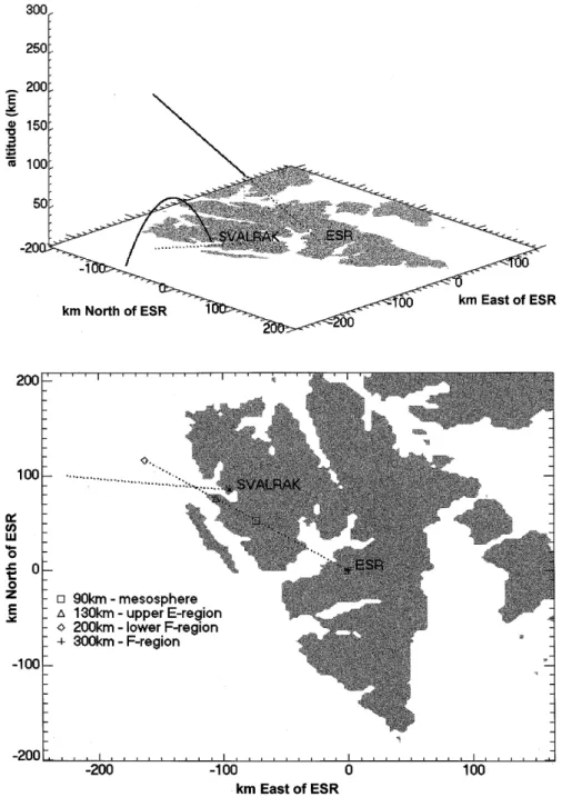
The ISBJéRN I payload was ¯own on 20 November at 1732 UT and successful measurements were made in the height interval 50±71 km (Thrane et al., this issue). The positive ion probe (Blix et al., 1990), as the name suggests, determines the positive ion density, and this should not be confused with the electron density. In particular, at the time of year we shall present data from here, there is a strong likelihood that there was a signi®cant negative ion content at least up to the upper mesosphere. The ESR system was directed at low elevation (45°) and scanned in azimuth. The pointing directions were 265°, 270°, 285°, 300°, 315°, 330° and 345° with a dwell time of 2 min at each position. It is important to be able to visualise the geometry of the combined experiment in order to assess the assump-tions regarding homogeneity and stationarity that will be implicit in our conclusion. Figure 1 shows a 3-dimensional view: Svalbard is seen from the southwest with horizontal axes indicating distance in kilometers from ESR; the vertical axis indicates altitude in kilome-ters; the parabola indicates the measured trajectory of ISBJéRN I; the straight line extending from ESR is a typical beam (azimuth 300°) and is dotted in the region where clutter/interference makes measurements useless (see later); the dotted line on the ground indicates the footprint of the ESR beam. In Fig. 1, note that ESR measures at much longer ranges than indicated here, but we have chosen not to extend the plot upwards to the left for clarity. Figure 2 shows a plan view of the information in Fig. 1, and in particular, the points on the ESR beam where it intersects selected altitudes. Systems of the con®guration of ISBJéRN I are usually expected to attain higher altitudes in which case one can
see that the ESR measurement volume and the payload trajectory could be arranged to be very close. In our case, there was a spatial separation of around 100 km between the payload apogee and the lowest ESR volume. We shall see that conditions were geomagnet-ically quiet and that ESR failed to detect any substantial spatial structure in the plasma density during the period in question, and we shall use this as part of our justi®cation for presenting a composite ion density pro®le. While such plasma density measurements are commonplace at, for example, the EISCAT mainland site (69°N, 19°E), a database of such soundings does not, as yet, exist for Svalbard. Thus although this work will not present new physics, it is intended to contribute to establishing the status quo for the ionosphere at 80°N, 16°E.
ESR measurements
While it is unfortunate that there are diculties in measuring at low altitude (i.e. under 85 km as we shall see) with ESR and therefore determining true height pro®les, pointing the radar at a 45° elevation allows for a convenient portrayal of the results. In Figs. 3 and 4, we show the average electron density for the two periods of operation 1645±2300 UT on 19 November, 1997, and 1409±2010 UT on 20 November, 1997. The ®gures show plan views of the observed region with axes indicating horizontal distance from the ESR site. Since the elevation was very nearly 45°, the horizontal range from ESR is equal to the altitude. Stating that these are plots of electron density is, however, not quite true; equivalent electron densities have been calculated from
Fig. 1. Three-dimensional representation of the measurement geometry. The ``¯oor'' depicts Svalbard seen from the southwest with horizontal axes indicating distance in km from ESR. The vertical axis indicates altitude in km; the parabola indicates the measured trajectory of ISBJéRN I. The straight line extending from ESR is a typical beam (azimuth 300°) and is dotted in the region where clutter/interference makes measurements useless (see text). The dotted line on the ground indicates the footprint of the ESR beam. Landmasses are grey; sea is left white
Fig. 2. Two-dimensional representation of the measurement geometry. This is essen-tially a plan view of the previous ®gure, but indicates intersections of the ESR beam with selected altitudes. The apogee of ISBJéRN I was 70 km and is this repre-sented by the mid-point of the line extending west from SVALRAK
the backscattered power assuming the scattering process to be that of classical incoherent scatter (Lehtinen and Huuskonen, 1996). No account has been taken for possible presence of negative ions, a factor which may aect the signal especially below 95 km. Little is known
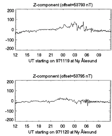
of negative ion concentration at such high latitudes and this in itself would be a worthy continuation of this kind of investigation. More importantly, though, clutter or interference of some kind manifests itself below 85 km as can be clearly seen by the ``trough'' in density at this horizontal range; All signals/closer to the radar than 85 km must be construed as artefact. It is interesting to note that this 85 km limit is independent of azimuth and this raises the question as to whether ESR is indeed aected by ground clutter, which we would expect to exhibit azimuth dependence. In the ®gures, we have attempted to show the average nature of the degree of ionisation on these two days. Obviously short-term variations may have occurred which we have subse-quently averaged out. In practice, some sporadic E had been observed on 19 November, but this was less prevalent on 20. The conditions otherwise varied little as can be con®rmed by that absence of signi®cant geo-magnetic activity depicted by Fig. 5, in which the two panels show the magnetometer records (z-component) for Ny AÊlesund (location of SVALRAK) for the two days in question. Furthermore, note that the ionosphere is not sunlit during this period. The solar (10 cm) ¯ux was 86.5 on the launch day, with a mean Ap of 2. Obviously, the individual soundings at 2 min resolution that have been averaged to construct Figs. 3 and 4 are also available, and in particular that nearest in time and space to ISBJéRN I; we shall defer presentation of this individual sounding until later.
Fig. 3. Average electron density (or rather backscattered power calculated as electron density assuming scattering process is incoher-ent scatter) for 19 November, 1997. Axes denote horizontal distance from ESR. The radar operated at an elevation of 45° such that the horizontal range on the plot is identical to the measurement altitude. Period of measurement was 1645-2300 UT. Contours are labelled in log10(electrons per m3)
Fig. 4. As for Fig. 3 but for 20 November, 1997. Period of measurement was 1409-2010 UT
Fig. 5. Z-component magnetometer records for Ny AÊlesund for 19 (top) and 20 (bottom) November, 1997. On each day, the record starts at 12 UT and extends for a 24-h period
ISBJéRN measurements
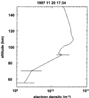
As described, the current ¯owing through the positive ion probe may be combined with the probe cross section to estimate the positive ion density. To illustrate the nature of this current we show the probe results in Fig. 6. Although plotted on a logarithmic scale (because the ¯uctuation amplitude tends to increase exponentially with height due to the increasing plasma density), we see that there is essentially a linear increase of positive ion
density through the height range of the observation. The reliability of the calculation has been established by, for example, Hall et al. (1985). Had electron density been measured in situ by the same payload, the dierence between this and the positive ion probe would have represented the negative ion density (in order to preserve quasi neutrality of the gas). The ¯uctuations in the signal may be used to determine turbulence parameters, but we shall not address this kind of physics here. The resulting positive ion densities were determined to be 2 ´ 109m)3 at 50 km increasing almost linearly to
2.4 ´ 109m)3 at 70 km. The uncertainties due to
instrumental noise and ion capture cross section amount to a factor 2.
Composite results
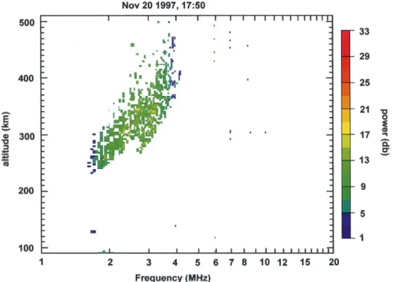
While we have considerable con®dence in the ion probe determinations of ion density, ESR calculations depend on a ``system constant'' to establish absolute values of plasma density. Furthermore, the nature of ESR operation, which entailed real-time transfer of plasma parameters onto the Internet in order to contribute to launch criteria for ISBJéRN I, precluded recording of uncertainties. We have attempted to circumvent this problem, however, by introducing ionosonde data (University of Leicester ionosonde) and scale the ESR pro®les accordingly. Some minutes prior to launch, a sporadic E (Es) layer had been observed but as ISBJéRN I attained apogee this had faded and only a remnant remained. The ionogram subsequent to the ISBJéRN I ¯ight is shown in Fig. 7. In the usual way (e.g. Hargreaves, 1992) we may convert the ionogram
Fig. 6. Positive ion probe current for ISBJéRN I. The absolute units are unimportant; the general increase in current from 55 to 70 km corresponds to a linear increase in electron density from 2 ´ 108m)3 to 7 ´ 108m)3
Fig. 7. Ionogram for 1750 UT on 20 November, 1997. The small area of signal at about 125 km virtual height is con-sidered to represent the rem-nants of an Es layer observed some 25 min earlier. The same feature is visible on the preced-ing ionogram at 1735 UT (not included here). The colour cod-ing denotes signal strength
critical frequencies to electron densities, which in turn indicate 5 ´ 1010m)3 at 260 km and 1.4 ´ 1011 m)3 at
380 km. Further to our discussion on the stationarity of the ionosphere during the evening of 20 November, we have noted little change in the F-region critical frequency, although a degree of variable Es was present.
Figure 8 depicts measurements from all three instru-ments on the same axes. The average of the factors required to scale the ESR plasma density pro®le to the ionosonde measurements was then determined, along with the standard deviation. The former was used to scale the ESR pro®le while the latter was used to determine a somewhat simplistic uncertainty. The iden-ti®cation of a minimum height of 85 km for useful observations by ESR at the time of the experiment via Figs. 4 and 5 and Hall (1997), leads to the rejection of data below 85 km. The reader is asked to recall that the ESR measurements presented here were accumulated as a result of a telescience service to the launch of ISBJéRN I and future D-region investigation will entail a more stringent approach to error treatment. Furthermore, future combination of ionosonde sound-ings with ESR pro®les will help to determine the ESR system constant with more con®dence rendering the inclusion of ionosonde measurements unnecessary. Nevertheless, it is hoped that the results presented here are of use to future ESR operations as a reference. Combining the ionosonde data with the ESR pro®le in this way and interpolating between the ion probe pro®le and the incoherent pro®le we arrive at Fig. 9. The pro®le in Fig. 9 may either be interpreted as a positive ion density pro®le, or, if we assume no negative ions, an electron density pro®le. It is tempting to identify the ledge at around 90 km as the negative ion shelf, but the authors feel this is a dangerous interpretation with so
little data. It is conceivable that future investigation could establish negative ion density in ways similar to Hall et al. (1985), or Hall et al. (1998).
Conclusion
Despite not fully understood problems with ESR for measurements in the mesosphere, and the unexpectedly low apogee of the ISBJéRN I payload, we have determined a pro®le for positive ion density through the mesosphere and up to the F-region for the evening of 20 November, 1997, over Svalbard. We have deter-mined, to some degree, the minimum measurement altitude for ESR at the time of writing and also the relation between electron densities indicated by the ESR standard analysis and ionosonde measurements. Al-though only an exploratory investigation has been reported here, it is of value for future measurements, both ground-based and in situ. The need to understand and alleviate the problems of low altitude ESR mea-surements have been identi®ed, as has the need for combined in situ and ground-based measurements for mapping the negative ion presence in the mesosphere and lower thermosphere at high latitude.
Acknowledgements. The authors are indebted to the Director and sta of EISCAT for operating the facility and supplying the data. EISCAT is an International Association supported by Finland (SA), France (CNRS), the Federal Republic of Germany (MPG), Japan (NIPR), Norway (NFR), Sweden (NFR) and the United Kingdom (PPARC). The authors are also indebted to The University of Leicester for provision of ionosonde data. The authors thank the Magnetometer Group of the Auroral Observa-tory, Tromsù, Norway for provision of magnetometer data.
Topical Editor F. Vial thanks M. Friedrich and another referee for their help in evaluating this paper.
Fig. 8. All plasma density measurements for the launch of ISBJéRN I on 20 November, 1997. The solid line represents the ESR measurement; the dotted line represents the ISBJéRN I measurement and the two stars the ionosonde measurement
Fig. 9. Final composite plasma density pro®le for ISBJéRN I launch. See text for details
References
Blix, T. A., E. V. Thrane, and é. Andreassen, In situ measurements of the ®ne-scale structure and turbulence in the mesosphere and lower thermosphere by means of electrostatic positive ion probes, J. Geophys. Res., 95, 5533±5548, 1990.
Hall, C., T. A. Blix, A. Brekke, M. Friedrich, T. L. Hansen, S. Kirkwood, J. RoÈttger, and E. V. Thrane, MAP/WINE electron density pro®les in the D- and E-regions: a comparison of EISCAT, PRE and rocket data, Proc. 7th ESA Symposium (ESA SP-229), 279±284, 1985.
Hall, C., T. Devlin, A. Brekke, and J. K. Hargreaves, Negative ion to electron number density ratios from EISCAT mesospheric spectra, Phys Scripta, 37, 413±418, 1988.
Hall, C. M., Feasibility of using EISCAT Svalbard Radar (ESR) in conjunction with in situ measurements, Auroral Observatory
Technical Report 1/97, University of Tromsù, Tromsù, Norway, 1997.
Hargreaves, J. K., The solar terrestrial environment, Cambridge University Press, Cambridge, UK, 1992.
Lehtinen, M. S., and A. Huuskonen, General incoherent scatter analysis and GUISDAP, J. Atmos. Terr. Phys., 58, 435±452, 1996.
Thrane, E. V., T. A. Blix, and K. R. Svenes, Irregular structures observed in the nighttime polar D-region, Ann. Geophysicae, this issue, 1999.
Wannberg, U. G., I. Wolf, L.-G. Vanhainen, K. Koskenniemi, J. RoÈttger, M. Postila, J. Markkanen, R. Jacobsen, A. Stenberg, R. Larsen, S. Eliassen, S. Heck, and A. Huuskonen, The EISCAT Svalbard radar, a case study in modern incoherent scatter radar system design, Radio Sci., 32, 2283± 2307, 1997.