HAL Id: hal-00316982
https://hal.archives-ouvertes.fr/hal-00316982
Submitted on 1 Jan 2003
HAL is a multi-disciplinary open access
archive for the deposit and dissemination of
sci-entific research documents, whether they are
pub-lished or not. The documents may come from
teaching and research institutions in France or
abroad, or from public or private research centers.
L’archive ouverte pluridisciplinaire HAL, est
destinée au dépôt et à la diffusion de documents
scientifiques de niveau recherche, publiés ou non,
émanant des établissements d’enseignement et de
recherche français ou étrangers, des laboratoires
publics ou privés.
Assessing the performance of the Cretan Sea ecosystem
model with the use of high frequency M3A buoy data set
G. Triantafyllou, G. Petihakis, I. J. Allen
To cite this version:
G. Triantafyllou, G. Petihakis, I. J. Allen. Assessing the performance of the Cretan Sea ecosystem
model with the use of high frequency M3A buoy data set. Annales Geophysicae, European Geosciences
Union, 2003, 21 (1), pp.365-375. �hal-00316982�
Annales
Geophysicae
Assessing the performance of the Cretan Sea ecosystem model with
the use of high frequency M3A buoy data set
G. Triantafyllou1, G. Petihakis1, and I. J. Allen2
1Institute of Marine Biology of Crete, P.O. Box 2214, Iraklio, 71003 Crete, Greece 2Plymouth Marine Laboratory, Prospect Place, West Hoe, Plymouth, PL1 3DH, UK
Received: 2 July 2001 – Revised: 22 April 2002 – Accepted: 12 June 2002
Abstract. During the Mediterranean Forecasting System
Pi-lot Project a buoy was deployed in the Cretan Sea and for the first time high-frequency physical and biogeochemical data were collected over an extended period, providing a unique opportunity for the evaluation of an ecosystem model. The model both tuned and validated in the Cretan Sea in the past, is explored and quantified. In addition, the optimal parameter set is determined while the effects of high-frequency forcing are explored. The model results are satisfactory, especially at the upper part of the water column, while the inability of 1-D modelling in fully exploring the hydrodynamics of the partic-ular area is depicted and further developments are suggested.
Key words. Oceanography; general (numerical modeling)
– Oceanography; biological and chemical (ecosystems and ecology)
1 Introduction
Heavily populated coastal areas bound the Mediterranean Sea. The economies of these regions are highly dependent on fishing, transportation, recreation and other industries, which in turn depend on a healthy coastal environment. Predict-ing the behaviour of the marine environment is an essen-tial part of the management of marine resources under an-thropogenic stress. Therefore, It is an essential requirement for the marine science community to determine the poten-tial time-scales of predictability of the marine ecosystem if an operational coastal ocean environmental monitoring and forecast system is to be developed. Such a system would provide estimates of the changes in both the physical and the biogeochemical marine environments and an enhanced understanding of the marine ecosystem, essential to guiding resource management. Additionally, it would form an early warning system of potentially harmful ecological events and aid the formulation of cost-effective preventive and remedial Correspondence to: G. Triantafyllou (gt@imbc.gr)
measures. Towards these issues an existing ecosystem model both tuned and validated in the Cretan Sea (Triantafyllou et al., 2002), is explored and its performance is quantified. As a first step historical and recent data sets are used to exploit the model to determine the optimal parameter set. The par-ticular ecosystem model was chosen due to its generic na-ture in response to the physicochemical environment within which it is placed. With all significant biological pathways in the modelled system included, the model can respond to the physical and chemical forcing in a way that is at least qualitatively correct under a wide range of conditions.
In this study, high-frequency forcing data from the POSEI-DON system (Soukissian et al., 1999) and the M3A buoy are used and compared with climatological forcing, in an attempt to investigate whether the performance of the ecosystem model is enhanced. High-frequency forcing model results are further validated with in situ data of nutrients and chlorophyll collected during maintenance trips. Finally, high-frequency data of chlorophyll, nitrate, oxygen and temperature during M3A deployment is hindcast with model results.
2 Materials and methods
2.1 Study area
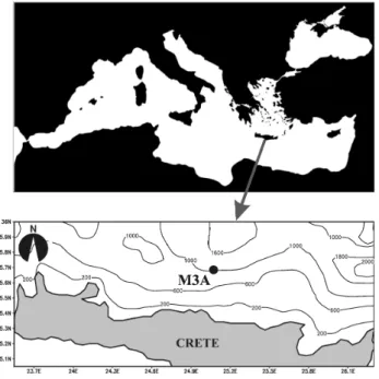
The area under study is the M3A mooring site located at 35◦07007.5400N, 24◦59044.6600E in the Cretan Sea, north of Heraklion, with a depth of 1100 m (Fig. 1). The open char-acter of the area in conjunction with the significant distance from the north coast of Crete (21 miles) ensures that there is no influence from land activities in the functioning of the specific ecosystem. The simulation period is the M3A de-ployment period starting from 30 January 2000 until 20 April 2001.
The Cretan Sea at the eastern part of the Mediterranean is dominated by multiple scale circulation patterns. The hydrological structure is complex and is characterised by mesoscale variability. It is an area of deep-water formation
Fig. 1. Map of M3A mooring.
with a sporadic and episodic formation of intermediate wa-ter occurring predominantly in the late winwa-ter. From spring through to late autumn/ early winter the region is thermally stratified to a depth of 50–70 m. The ecosystem of the outer Cretan Sea has two different modes of operation. During pe-riods of stratification it exhibits a microbial food web, when small phytoplankters dominate, taking advantage of their su-perior surface-to-volume ratio and a considerable portion of the total organic pool is in the form of detritus. Phospho-rus is thought to be the limiting nutrient for phytoplankton and bacterial growth (Becacos-Kontos, 1977; Berland et al., 1980; Krom et al., 1991, 1992; Thingstad and Rassoulzade-gan, 1995) with very low concentrations even below the eu-photic zone at 200 m. Nutrients are recycled in the top lay-ers with a prominent P limitation of both phytoplankton and bacteria, and high surface concentrations and vertically de-creasing gradients of DOP and DOC. During this mode very little energy is passed to the higher trophic layers and to the benthos. When the thermocline erodes the system switches into the classical mode during which trapped nutrients find their way to the euphotic zone, initiating a new production bloom and biomass distribution, being linearly ordered ac-cording to trophic levels along which the organisms increase sequentially in size (Smetacek and Pollehne, 1986).
The variability observed in biogeochemical parameters is due to the complex hydrological structure characterised by eddies interconnected with jets without defined time scales (Balopoulos, 1996). These features are important because they can transport, entrap and disperse chemicals, particu-late matter, small organisms, heat, etc., while they signifi-cantly modify the vertical mixing patterns in an area, creat-ing among other phenomena zones of upwellcreat-ing and down-welling that in turn can have a major effect on the biological
productivity (Krom et al., 1993). Those structures, in con-junction with the presence of transient Mediterranean water (TMW), a mass rich in nutrients and poor in oxygen, can drastically alter the chemical conditions of the intermediate layers of the entire south Aegean (Theocharis et al., 1999), acting as a nutrient source to the euphotic zone or as sinks for organic material to the deeper layers.
2.2 M3A data set
One of the innovations of the MFSPP project and the deploy-ment of the M3A buoy was the collection for the first time of high-frequency physical and biogeochemical data over an extended period in the outer Cretan Sea. Previous studies in this region were conducted on a seasonal time-scale, which, in the case of oligotrophic systems, may prove to be inad-equate in revealing the ecosystem dynamics since the tem-poral scales must be considered according to the biological time scales of growth (or generation time), which are rather short (Abbott, 1993). The M3A buoy provides 3-h measure-ments of temperature, chlorophyll-a, nitrate and oxygen, at various depths giving a unique opportunity for hindcasting modelling of the Cretan Sea ecosystem. The locations of the CTD and CT sensors were at 40, 60, and 90 m at line 2 and at 150, 250, 350 and 500 m at line 1. The chlorophyll-a and oxygen sensors were deployed at 40, 65, 90 and 115 m and the nitrate sensor at 45 m. A detailed description of the struc-ture and setup of the three moorings comprising the M3A array are presented in Nittis et al. (2003). Chlorophyll-a, dissolved oxygen and nitrate data were post-calibrated using in situ bottle measurements. The calibration coefficients for the M3A sensors were calculated separately for each period between maintenance cruises, using the reference data col-lected during each re-deployment when all sensors had been cleaned (Nittis et al., 2003).
2.3 Ecosystem model
In this study the model used is a highly portable coupled physical biogeochemical water column model (Allen et al., 1998) adapted for the oligotrophic Cretan Sea (Triantafyllou et al., 2002). The biogeochemistry is based on the European Regional Seas Ecosystem Model (ERSEM) (Baretta et al., 1995), while the physics are provided by a one-dimensional version of the Princeton Ocean Model (Blumberg and Mel-lor, 1978).
A turbulence closure model (Mellor and Yamada, 1982) determines the vertical temperature, turbulent kinetic energy, and diffusion coefficient profiles generated by a surface heat flux, salinity and wind stress. Heat transfer is assumed to be via vertical diffusion processes. A background viscosity parameterises other mixing processes (e.g. internal waves). The physical sub-model, in addition, to transport describes irradiance, temperature, and sea surface boundary condi-tions. The solar radiation is provided to the biogeochemical model as photosynthetically available radiation (PAR) pene-trating the water column and becoming extinct with
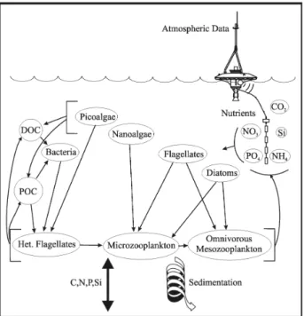
increas-Fig. 2. Ecosystem model food web.
ing depth, according to an extinction coefficient calculated at each time step from the concentrations of primary producers, detritus, bacteria and inorganic suspended matter (Zavatarelli et al., 2000).
The basis of the biogeochemical model consists of state variables with a functional group, approach where organisms are grouped according to their trophic level subdivided ac-cording to size classes or feeding method. Two sub-models describe the ecosystem, one for the pelagic and another one for the benthic ecosystem, coupled in terms of carbon and nutrients. The pelagic sub-model includes all the important components, such as nutrient pools, oxygen, phytoplankton, mesozooplankton, microzooplankton, bacteria and detritus. Although the full benthic sub-model depicts a rather diverse system, in this study, due to the depth (> 1000 m) and the oligotrophic nature of the system, benthic processes are de-scribed by the simple first order benthic returns module. Ac-cording to this the detritus falling into the benthos is added in both the particulate and dissolved benthic pools from which a proportion of the total carbon (5% of the particulate and 10% of the dissolved fraction) is remineralised and returned to the water column as CO2. The nutrient components of
these forms of detritus follow the same proportions with 10% of the remineralised nitrogen added to the nitrate and the rest 90% to the ammonium pools. The remineralised phosphorus is fluxed to the inorganic phosphate pool.
The model food web is modified from the standard ERSEM version 11 (Baretta et al., 1995), according to the characteristics of the ecosystem under study as they have been revealed from literature and analysis of in situ data (Azov, 1991; Stergiou et al., 1997; Tselepides and Poly-chronaki, 1996) (Fig. 2). Thus, phytoplankton is
com-posed of four groups with diatoms and flagellates being grazed by microzooplankton and omnivorous mesozooplank-ton, nanoalgae grazed by microzooplankmesozooplank-ton, while picoalgae and bacteria are grazed by heterotrophic nanoflagellates. To take into account the importance of bacterial nutrient limita-tion and the role of dissolved organic material in this olig-otrophic system, a modified version (Allen et al., 2002) of the standard ERSEM pelagic sub-model bacteria (Baretta-Bekker et al., 1998; Baretta-(Baretta-Bekker et al., 1995) was used.
The 1-D Cretan Sea ecosystem model (Triantafyllou et al., 2002) which was used has a vertical resolution of 40 lay-ers and total depth of 1100 m, with a finer resolution at the euphotic zone (0–150 m every 10 m). It was forced with six hourly wind speed, humidity, cloud cover and air temperature data obtained from ECMWF. Incident sea surface radiation is calculated from the latitude modified by the cloud cover data using the methods of Patsch (1994), while the extinction co-efficient was parameterised according to the measured depth of 1% incident solar irradiance (80–90 m) (Gotsis-Skretas et al., 1999; Ignatiades et al., 1995; Psarra et al., 2000). In this study the model was also forced with high-frequency wind speed and air temperature data for the computation of wind stresses (Hellermann and Rosenstein, 1983) and relaxed to mean monthly sea surface temperature and salinity obtained from a POSEIDON buoy (Soukissian et al., 1999) located 10 miles south of M3A during the period of the M3A deploy-ment (January 2000–April 2001).
2.4 Optimal parameter set
The optimal parameter set for the autotrophic and het-erotrophic groups in the model are given in Tables 1 and 2, respectively. The maximum specific uptake rate in all phy-toplankton groups was lowered to avoid excess production of dissolved organic carbon (DOC) and subsequent growth of bacteria, which will compete for nutrients with phyto-plankton. Faster rates of small cells are, however, retained. Oligotrophic phytoplankton was shown to grow at rates of 0.5–2 d−1, significantly faster than bacterioplankton (Laws et al., 1987), as expected if one considers that in such sys-tems the heterotrophic biomass exceeds that of autotrophs. In oligotrophic systems phytoplankters exhibit a dormant be-haviour where photosynthesis rates are minimum, relying on a chance encounter with nutrient patches to revive their pho-tosynthetic mechanism (Smetacek and Pollehne, 1986). In addition the maximum N:C and P:C ratios for phytoplankton have been altered to restrict the luxury uptake of nutrients.
In the microzooplankton module some food preference factors have been changed to account for the fact that di-noflagellates, unlike standard ERSEM V.11 where they were considered inedible, are parameterised as a food source for omnivorous microzooplankton. The bacterial specific uptake rate was significantly lowered, in order to reduce the bacterial growth rate in the range of 0.006–0.086 (d−1), as suggested by Turley et al. (2000) and Pedros-Alio et al. (1999). Finally the assimilation efficiency was also lowered, simulating an average bacterial growth efficiency of 5–20% (Carlson and
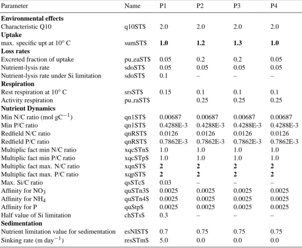
Table 1. Parameters of the phytoplankton functional groups. P1 = diatoms, P2 = nanoalgae, P3 = picoalgae, and P4 = dinoflagellates. The parameters that have been changes from the standard ERSEM version 11 are indicated in bold. Parameter names used follow the nomenclature described in Blackford and Radford (1995)
Parameter Name P1 P2 P3 P4
Environmental effects
Characteristic Q10 q10ST$ 2.0 2.0 2.0 2.0
Uptake
max. specific upt at 10◦C sumST$ 1.0 1.2 1.3 1.0
Loss rates
Excreted fraction of uptake pu eaST$ 0.05 0.2 0.2 0.05
Nutrient-lysis rate sdoST$ 0.05 0.05 0.05 0.05
Nutrient-lysis rate under Si limitation sdoST$ 0.1 – – – Respiration
Rest respiration at 10◦C srsST$ 0.15 0.1 0.1 0.1
Activity respiration pu raST$ 0.25 0.25 0.25
Nutrient Dynamics
Min N/C ratio (mol gC−1) qn1ST$ 0.00687 0.00687 0.00687 0.00687
Min P/C ratio qn1ST$ 0.4288E-3 0.4288E-3 0.4288E-3 0.4288E-3
Redfield N/C ratio qnRST$ 0.0126 0.0126 0.0126 0.0126
Redfield P/C ratio qnRST$ 0.7862E-3 0.7862E-3 0.7862E-3 0.7862E-3
Multiplic fact min N/C ratio xqcSTn$ 1.0 1.0 1.0 1.0
Multiplic fact min P/C ratio xqcSTp$ 1.0 1.0 1.0 1.0
Multiplic fact max. N/C ratio xqnST$ 2 2 2 2
Multiplic fact max. P/C ratio xqpST$ 2 2 2 2
Max. Si/C ratio qsSTc$ 0.03 – – –
Affinity for NO3 quSTn3$ 0.0025 0.0025 0.0025 0.0025
Affinity for NH4 quSTn4$ 0.0025 0.0025 0.0025 0.0025
Affinity for P quStp$ 0.0025 0.0025 0.0025 0.0025
Half value of Si limitation chSTs$ 0.3 – – –
Sedimentation
Nutrient limitation value for sedimentation esNIST$ 0.7 0.75 0.75 0.75
Sinking rate (m day−1) resSTm$ 5.0 0.0 0.0 0.0
Ducklow, 1996; Kirchman et al., 1991; Pedros-Alio et al., 1999; Turley et al., 2000).
3 Results and discussion
3.1 Hindcast experiments
3.1.1 Temperature
Temperature simulations plotted against in situ measure-ments for the 40, 60, 90 and 150 m depths are shown in Fig. 3. Stratification started approximately at the middle of April, reaching the highest subsurface values towards the end of October, and the location of the thermocline lay between 40 and 65 m. From November onwards a gradual mixing of the thermocline into deeper layers occurred until it dis-appeared in early January (Nittis et al., 2003). The bottom of the seasonal thermocline was at 50–70 m and, thus, the signal of the annual cycle of heating and cooling is hardly detected below that depth. At 40 m the model results follow very closely the field values, with minimum temperatures in March and Maximum in October. The large variability in
the in situ values of almost 4◦C within a few days after June 2000 may be associated with changes in the eddy structure of the region. While the variation during October 2000 and December 2000 to January 2001 was coincident, with sig-nificant movements of the mooring line (Nittis et al., 2003). At 65 m the simulated temperature follows the general trend in the data, but fails to reproduce the observed variability. This variability is less pronounced than at 40 m and can be ascribed to similar processes. At both 90 m and 150 m there is no significant seasonality in the data and the model repro-duces the observations.
3.1.2 In situ validation
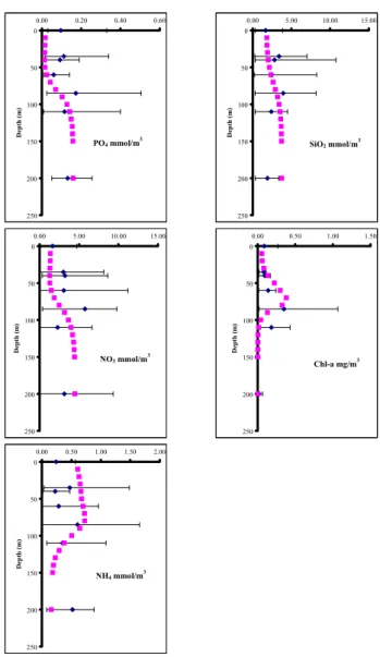
The in situ data collected during the maintenance trips was compared with model results for nutrients and chlorophyll. Figure 4 shows simulated annual mean values plotted against depth, along with mean in situ concentrations for the period from 30 January 2000 until 19 April 2001, while range bars indicate minimum and maximum measured values. Model results are generally in good agreement with the observed in situ data in the whole water column, although the field data exhibits a substantial variability in almost all parameters.
Table 2. Parameters of microzooplankton functional groups and bacteria. Z5 = microzooplankton, Z6 = heterotrophic flagellates and B1 = bacteria. The parameters that have been changed from the standard ERSEM version 11 are indicated in bold. Parameter names follow the nomenclature described by Blackford and Radford (1995)
Parameter Name B1 Z6 Z5
Environmental effects
Characteristic Q10 q10ST$ 2.95 2.0 2.0
Half oxygen saturation chrSTo$ 0.3125 7.8125 7.8125 Uptake
Half saturation value chuSTc$ 30.0 250 200
Max. spec uptake rate 10◦C sumST$ 0.8 5.0 1.2
Availability of P1 for ST suP1 ST$ – 0.0 1.0
Availability of P2 for ST suP2 ST$ – 0.0 0.4
Availability of P3 for ST suP3 ST$ – 0.4 0.0
Availability of P4 for ST suP4 ST$ – 0.0 1.0
Availability of Z5 for ST suZ5 ST$ – 0.0 1.0
Availability of Z6 for ST suZ6 ST$ – 0.2 1.0
Availability of B1 for ST suB1 ST$ – 1.0 0.0
Selectivity mindfoodST$ – 100 30
Loss rates
Assimilation efficiency puST$ 0.25 0.4 0.5
Assimilation efficiency at low temp puST0$ 0.2 – –
Excreted fraction of uptake pu eaST$ – 0.5 0.5
Excretion
Fraction of excretion production to DOM pe R1ST$ – 0.5 0.5 Mortality
Oxygen dependent mortality rate sdST0$ – 0.25 0.25 Temperature independent mortality sdST$ 0.001 0.05 0.05 Respiration
Rest respiration at 10◦C srsST$ 0.01 0.02 0.02
Nutrient Dynamics
Max. N/C ratio qnSTc$ 0.0208 0.0167 0.0167
Max. P/C ratio qpSTc$ 0.00208 0.00167 0.00167
Field data (phosphate, nitrate, ammonia and silicate) in-dicate the presence of a weak nutracline at 80 m, which is successfully reproduced, although more pronounced in the model results. In the top 100 m the model phosphate values are close to the minimum measured concentrations, with the data fit improving below 100m. It should be noted that com-pared to the CINCS data set for the same region (Tselepides et al., 2000) (April 1994 – July 1996), phosphate values dur-ing the M3A deployment period are significantly higher. Ni-trate exhibits a similar picture to phosphate with model con-centrations close to the lower end of the range of in situ data. Once again, M3A nitrate concentrations are higher than the CINCS data and exhibit significantly higher variability at all depths. Simulated silicate and ammonia concentrations lie within the variability of measured concentrations. The maxi-mum measured chl-a values at 80m are indicative of the deep chlorophyll maximum (DCM), a characteristic of the area (Tselepides et al., 2000), which is reproduced by the model at a slightly shallower depth. This is due to the fact that in the model the DCM coexists with the maximum biomass, while the analysis of the in situ data shows that the DCM is deeper compared to the biomass or cell count maximum
(Psarra et al., 2000), indicating an elevated chlorophyll per cell content at deeper layers. The model fails to reproduce chlorophyll in the deeper parts of the water column below 10 m, where small chlorophyll levels are detected even down to 200–400 m due to wind mixing, as has been suggested by Tselepides and Polychronaki (1996).
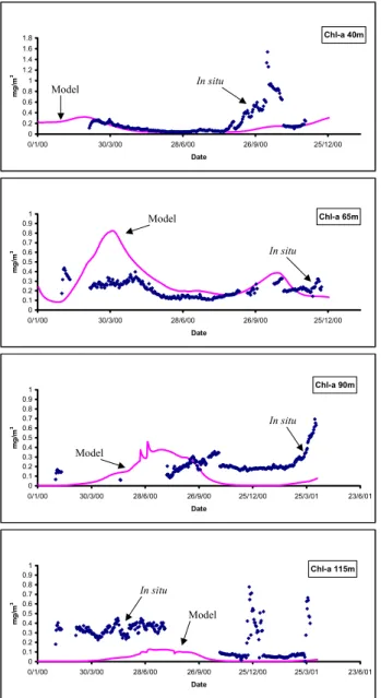
3.1.3 Chlorophyll
Figure 5 shows the simulated chl-a against the in situ flu-orometer derived concentrations. Model results are very close to the measured concentrations at 40 m, with the ex-ception of the period from 22 August 2000 until 29 October 2000, which can be attributed to biofouling of the sensor and the vertical displacement of the mooring line (Nittis et al., 2003). During this period the comparison of model and data is meaningless. This argument is strengthened by the fact that after 31 October 2000, the measured chl-a concentra-tions are once more very close to the model simulation.
At 65 m the model overestimated chlorophyll during March and April 2000, producing a peak at the end of March due to intense mixing. For the rest of the deployment period the simulation is very good, closely following the measured
Temperature 40m 10 12 14 16 18 20 22 24 0/1/00 30/3/00 28/6/00 26/9/00 25/12/00 Date oC Temperature 65m 10 11 12 13 14 15 16 17 18 19 20 0/1/00 30/3/00 28/6/00 26/9/00 25/12/00 Date oC Temperature 90m 10 11 12 13 14 15 16 17 18 19 20 0/1/00 30/3/00 28/6/00 26/9/00 25/12/00 Date oC Temperature 150m 10 11 12 13 14 15 16 17 18 19 20 0/1/00 30/3/00 28/6/00 26/9/00 25/12/00 Date oC Model Model Model Model In situ In situ In situ In situ
Fig. 3. Validation of model temperature with CTD measurements at 40, 65, 90 and 150 m.
concentrations, producing a peak in October and minimum values in February and August 2000.
At 90 m field data was unavailable for the first seven months due to sensor problems. For the rest of the de-ployment period the model, although following the measured trend, systematically produced lower concentrations. Analo-gous model behaviour is observed at 115 m, where there is an underestimation of Chl-a, although differences appear signif-icant only during the first seven months. This poor behaviour of the model may partly be due to the use of a constant C:Chl ratio at all depths. It is well documented that there is a com-mon trend of an increase in chlorophyll-a and other light har-vesting pigments as growth irradiance decreases (Dubinsky, 1992; Estrada, 1985; Estrada et al., 1993; Gasol et al., 1997; Venrick, 1990). However, there is a rather wide range of C:Chl values suggested by researchers for different
environ-PO4 mmol/m3 0 50 100 150 200 250 0.00 0.20 0.40 0.60 D ept h ( m ) NO3 mmol/m3 0 50 100 150 200 250 0.00 5.00 10.00 15.00 D ept h ( m ) NH4 mmol/m3 0 50 100 150 200 250 0.00 0.50 1.00 1.50 2.00 D ept h ( m ) SiO2 mmol/m3 0 50 100 150 200 250 0.00 5.00 10.00 15.00 D ept h ( m ) Chl-a mg/m3 0 50 100 150 200 250 0.00 0.50 1.00 1.50 D ept h ( m )
Fig. 4. Validation of model Phosphate, Nitrate, Ammonia, Silicate and Chl-a with in situ data obtained during maintenance trips. All sampling measurements at a particular depth are treated as repli-cates and averaged. Range bars are used to indicate variability (min-imum and max(min-imum values).
ments, which confuses the parameterisation issue. A variable C/Chl ratio of decreasing values with increasing depth would improve the simulations at the deeper layers. An additional further source of discrepancy may arise from the calibration of the data, since there is a wide variation even within three days in the in situ measurements.
3.2 Oxygen
The dissolved oxygen sensors only gave reliable data during the first six months of the buoy deployment and then failed at the beginning of July 2000 (Fig. 6). At 40 m model results generally underestimate the oxygen concentration, except at the end of March 2000. Since the region is one of low pro-ductivity, this discrepancy can probably be ascribed to the fact that the model overestimates temperature at that depth. A
Chl-a 40m 0 0.2 0.4 0.6 0.8 1 1.2 1.4 1.6 1.8 0/1/00 30/3/00 28/6/00 26/9/00 25/12/00 Date mg /m 3 \ Chl-a 65m 0 0.1 0.2 0.3 0.4 0.5 0.6 0.7 0.8 0.9 1 0/1/00 30/3/00 28/6/00 26/9/00 25/12/00 Date mg /m 3 Chl-a 90m 0 0.1 0.2 0.3 0.4 0.5 0.6 0.7 0.8 0.9 1 0/1/00 30/3/00 28/6/00 26/9/00 25/12/00 25/3/01 23/6/01 Date mg /m 3 Chl-a 115m 0 0.1 0.2 0.3 0.4 0.5 0.6 0.7 0.8 0.9 1 0/1/00 30/3/00 28/6/00 26/9/00 25/12/00 25/3/01 23/6/01 Date mg /m 3 Model In situ Model Model Model In situ In situ In situ
Fig. 5. Validation of model chlorophyll concentration with CTD measurements at 40, 65, 90 and 115 m.
better agreement between simulation and field data is found at 65 m and 115 m, where the temperature simulations have a better fit with data. At 65 m the maximum oxygen concentra-tions are found during April–May, which may be attributed to increased primary production, as evidenced by the Chl-a concentrations.
3.2.1 Nitrate
Although model results (Fig. 7) are within the right range of measured values, they do not closely follow the in situ vari-ability. The extreme high values measured at the beginning of the data set are due to an unsuccessful deployment during which the analyser was almost at the surface. The marked decrease in nitrate during mid-May, suggesting an increased activity of primary producers, cannot be explained by the
chl-Oxygen 40m 3.000 3.500 4.000 4.500 5.000 5.500 6.000 6.500 7.000 0/1/00 30/3/00 28/6/00 26/9/00 25/12/00 Date m l/l Oxygen 65m 3.000 3.500 4.000 4.500 5.000 5.500 6.000 6.500 7.000 0/1/00 30/3/00 28/6/00 26/9/00 25/12/00 Date m l/l Oxygen 115m 3.000 3.500 4.000 4.500 5.000 5.500 6.000 6.500 7.000 0/1/00 30/3/00 28/6/00 26/9/00 25/12/00 Date m l/l Model Model Model In situ In situ In situ
Fig. 6. Validation of model oxygen concentration with CTD mea-surements at 40, 65, and 115 m. Nitrate 45m 0 1 2 3 4 5 6 7 0/1/00 30/3/00 28/6/00 26/9/00 25/12/00 Date mmol /m 3 Model In situ
Fig. 7. Validation of model nitrate concentration at 45 m, compari-son of nitrate concentrations from nitrate analyzer and in situ mea-surements during maintenance trips.
a measurements at the 40 and 65 m layers, where concentra-tions are either unchanged or decreasing. The failure of the model to reproduce this effect can be attributed to the lack of lateral advection of nitrate through the system. The observed nitrate concentrations in winter are lower than might be ex-pected form previous studies. It should be noted that strong mixing events during winter were not observed during the deployment period. It has been suggested by Georgopou-los et al. (1989); Theocharis (1995); Theocharis et al. (1993) that such events may significantly affecting the biology of the
Chl-a 10m 0.000 0.020 0.040 0.060 0.080 0.100 0.120 0.140 0/1/00 19/2/00 9/4/00 29/5/00 18/7/00 6/9/00 26/10/00 15/12/00 3/2/01 Date mmo l/m 3 Chl-a 30m 0.000 0.020 0.040 0.060 0.080 0.100 0.120 0.140 0.160 0.180 0.200 0/1/00 19/2/00 9/4/00 29/5/00 18/7/00 6/9/00 26/10/00 15/12/00 3/2/01 Date mmo l/m 3 Chl-a 50m 0.000 0.100 0.200 0.300 0.400 0.500 0.600 0.700 0/1/00 19/2/00 9/4/00 29/5/00 18/7/00 6/9/00 26/10/00 15/12/00 3/2/01 Date mmo l/m 3 Chl-a 70m 0.000 0.200 0.400 0.600 0.800 1.000 1.200 0/1/00 19/2/00 9/4/00 29/5/00 18/7/00 6/9/00 26/10/00 15/12/00 3/2/01 Date mmo l/m 3 Climatology Climatology Climatology Climatology High Frequency High Frequency High Frequency High Frequency
Fig. 8. Model chlorophyll simulations at various depths with clima-tological and real-time forcing.
area.
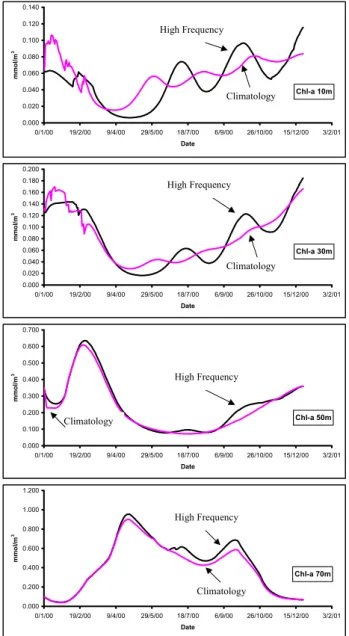
3.3 Sensitivity analysis, the response of the model to changes in forcing
The effects of changes in the atmospheric forcing upon the model behaviour were investigated by making two sepa-rate runs. In the first run, climatological wind forcing was used and the model was relaxed to climatological sea surface temperature, and salinity obtained from the Mediterranean Ocean Data Base database (Brasseur et al., 1996). For the second run, high-frequency wind forcing (half hour), for the period from 1 January 2000 until 3 February 2001, for the specific area, was obtained from the POSEIDON system, while the model was relaxed to mean monthly in situ sea surface temperature and salinity. The simulations of
chloro-phyll at the depths of 10, 30, 50 and 70 m from the two runs are shown in Fig. 8.
In the deeper layers, at 50 and 70 m, there are no signif-icant differences between the two runs, and the model pro-duces a spring and autumn bloom. At 50 m the spring bloom is observed during March, while at 70 m the spring bloom is observed during the end of April/beginning of May. In both layers the autumn bloom is shown during September– October.
However, in the upper layers (10 and 30 m), there are sig-nificant differences between the two runs, with more pro-nounced minimum and maximum chlorophyll concentrations in the run with the high-frequency data forcing, due to the diffusion of nutrients caused by the vertical mixing pro-cesses, which are much better described.
Thus, the model results indicate that the 1-D physical model only responds to sea surface forcing in the near sur-face layers and that the effect of high-frequency forcing data in the simulation of the ecosystem is only significant in the mixed layer. As mentioned above, the appearance of the Transition Mediterranean Water (TMW) at approximately 300–500 m, characterized by high nutrient and low oxygen concentrations in conjunction with the gyral features popu-lating the area, significantly affects the intermediate layers of the Cretan Sea. Thus, in the deeper layers of the euphotic zone, the ecosystem functioning is significantly affected by the advective processes, which cannot be described by the present model requiring a 3-D model.
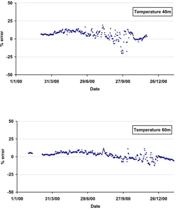
3.4 Model performance
The performance of the model is evaluated using the mis-fit error between modelled temperature (Fig. 9), Chl-a con-centrations (Fig. 10), and in situ data. The model underes-timates the temperature at 40 m by around 10–15% for most of the year, except in the autumn, when it is overestimated. At 65 m a similar trend is observed but the errors are smaller (5–10%). The model is consistently colder than the observa-tions, which implies that the buoyancy is weaker than reality and that vertical mixing may be overestimated. The imple-mentation of a surface heat flux formulation in the model may help to overcome these problems, as it would place the ecosystem model in a fully 3-D hydrodynamic environment. The data mismatch of chlorophyll is shown in Fig. 10. At 40 m the model consistently underestimates the data by 50– 100%, except during July, while at 65 m Chl-a is consistently overestimated by 50–100%, except during the bloom period, when the error is larger. There are a number of possible rea-sons for this discrepancy. The attenuation of light down the water column may be incorrect, and as previously, noted the vertical mixing may be wrong. Alternatively, the use of a fixed carbon to chlorophyll ratio in the model may cause this difference, with the ratio being underestimated in the near surface water and overestimated towards the bottom of the euphotic zone. The absence of phytoplankton biomass and primary production measurements precludes us from making further conclusions. However, it seems apparent that further
Temperature 40m -50 -25 0 25 50 1/1/00 31/3/00 29/6/00 27/9/00 26/12/00 Date % error Temperature 60m -50 -25 0 25 50 1/1/00 31/3/00 29/6/00 27/9/00 26/12/00 Date % error
Fig. 9. The percentage error (100*(Data-Model)/Data) for temper-ature at (a) 40 m and (b) 60 m.
work is required to improve the response of the phytoplank-ton model to low light environments. One possible solution is to implement a variable carbon-chlorophyll model, such as that of Geider et al. (1997).
The fit with nitrate at 45 m is shown in Fig. 11. In situ data and the model show a good fit in March and June/July, but overestimates the concentrations by 200–300% in between. The excess of nitrate in the spring may arise from the lack of horizontal advective processes in the model or through prob-lems with model phytoplankton uptake of nutrients and nutri-ent recycling mechanisms. Oxygen data (not shown) under-estimates the data by up to 5% at 40 m, 65 m and 115 m. This reinforces the previous conclusion that in a low productivity environment, the oxygen concentration is primarily temper-ature dependent.
Alternatively, data fits can be substantially improved by the implementation of a data assimilation scheme, such as the Ensemble Kalman Filter. This has been demonstrated for the M3A data set by Allen et al. (2003).
4 Conclusions
For the first time the oligotrophic ecosystem of the Cretan Sea has been monitored over an extended period of time, providing valuable information and a unique opportunity for ecosystem model application. The Cretan Sea ecosystem model developed during the MATER project when forced with real atmospheric data simulates very satisfactorily the
Chlorophyll 40m -300 -200 -100 0 100 200 300 1/1/00 31/3/00 29/6/00 27/9/00 26/12/00 Date % error Chlorophyll 65m -300 -200 -100 0 100 200 300 1/1/00 31/3/00 29/6/00 27/9/00 26/12/00 Date % error
Fig. 10. The percentage error (100*(Data-Model)/Data) for chlorophyll-a at (a) 40 m and (b) 60 m.
Nitrate 45m -300 -200 -100 0 100 200 300 1/1/00 31/3/00 29/6/00 27/9/00 26/12/00 Date % error
Fig. 11. The percentage error (100*(Data-Model)/Data) for nitrate at 45 m.
chl-a time series in the upper part of the water column as recorded by the fluorometers. Deeper down, close to the DCM the underestimation of the model concentrations can be attributed to the elevated cell chlorophyll content, a phys-iological adaptation to lower light conditions. A future mod-ification of the ecosystem model to account for this phe-nomenon, as well as the implementation of heat fluxes com-puted for the particular area, are considered necessary.
Although the in situ nitrate data are rather incomplete as a result of instrument malfunction such data, are, however, very important in these studies. Considering the phosphate limitation of the area high-frequency phosphate data from an autonomous instrument would provide significant informa-tion towards the improvement of the model.
Laboratory calibration of the fluorometric sensors is con-sidered crucial and necessary, in addition to the calibration with in situ data due to the significant variability of the chlorophyll concentrations in the samples in short-time pe-riods (2–3 days).
Due to its 1-D nature, the model does not include impor-tant processes of the particular area, such as horizontal ad-vection and vertical mixing arising from circulation patterns. Nevertheless, it provides a very successful numerical base for further development towards a 3-D forecasting ecosystem model and the implementation of assimilation techniques.
Acknowledgements. This work has been supported by Mediter-ranean Forecasting System Pilot Project MAS3-PL97-1608. The authors would like to thank A. Pollani for her substantial help, A. Eleftheriou for his constructive criticism during the preparation of this work, M. Eleftheriou for her help in editing this text, and K. Georgiou for software assistance.
Topical Editor N. Pinardi thanks T. Oguz and another referee for their help in evaluating this paper.
References
Abbott, M. R.: Phytoplankton patchiness: ecological implications and observation methods. In: Patch Dynamics, Lecture Notes in Biomathematics, (Eds) Levin, S. A., Powell, T. M., and Steele, J. H., Springer Verlag, Berlin Heidelberg, 307, 1993.
Allen, J. I., Blackford, J. C., and Radford, P. J.: An 1-D vertically resolved modelling study of the ecosystem dynamics of the mid-dle and southern Adriatic Sea, J. Marine Systems, 18, 265–286, 1998.
Allen, J. I., Somerfield, P. J. and Siddorn, J. R.: Primary and bac-terial production in the Mediterranean Sea: a modelling study, J. Marine Systems, (in press), 2002.
Allen, J. I., Ekenes, M. and Evensen, G.: An Ensemble Kalman Fil-ter with a complex marine ecosystem model: Hindcasting phyto-plankton in the Cretan Sea, Ann. Geophysicae, this issue, 2003. Azov, Y.: Eastern Mediterranean – a Marine Desert? EMECS’90,
23, 225–232, 1991.
Balopoulos, E. T.: PELAGOS, MAS2-CT93-0059, NCMR, Athens, 1996.
Baretta, J. W., Ebenhoh, W., and Ruardij, P.: The European Re-gional Seas Ecosystem Model, a complex marine ecosystem model, Netherlands, J. Sea Research, 33, 233–246, 1995. Baretta-Bekker, J. G., Baretta, J. W., Hansen, A. S., and Riemann,
B.: An improved model of carbon and nutrient dynamics in the microbial food web in marine enclosures, Aquatic microbial ecology, 14, 91–108, 1998.
Baretta-Bekker, J. G., Baretta, J. W., and Rasmussen, E.: The microbial foodweb in the European regional Seas Ecosystem Model, Netherlands, J. Sea Research, 33, 363–379, 1995. Becacos-Kontos, T.: Primary production and environmental factors
in an oligotrophic biome in the Aegean Sea, Marine Biology, 42, 93–98, 1977.
Blackford, J. and Radford, P.: A structure and methodology for Marine Ecosystem Modelling, Netherlands J. Sea Res., 33, 247– 260, 1995.
Berland, B., Bonin, D., and Maestrini, S.: Azote ou phosphore? Considerations sur le “paradoxe nutrionnel” de la Mer Mediter-ranee, Oceaonologica Acta, 3, 135–142, 1980.
Blumberg, A. F. and Mellor, G. L.: A Coastal Ocean Numerical Model. In: Mathematical Modelling of Estuarine Physics, (Eds) Sunderman, J. and Holtz, K., Proceedings of the International Symposium, Springer-Verlag Berlin, Hamburg, 203–214, 1978. Brasseur, P., Brankart, J.-M., Schoenauen, R., and Beckers, J.-M.:
Seasonal Temperature and Salinity Fields in the Mediterranean Sea: Climatological Analyses of an Historical Data Set, Deep Sea Rese., 43, 159–192, 1996.
Carlson, C. A. and Ducklow, H. W.: Growth of bacterioplankton and consumption of dissolved organic carbon in the Sargasso Sea, Aquatic Microbial Ecology, 10, 69–85, 1996.
Dubinsky, Z.: The functional and optical absorption cross-sections of phytoplankton photosynthesis. In: Primary Productivity and Biogeochemical Cycles in the Sea, (Eds) Falkowski, P. G. and Woodhead, A. D., Plenum Press, New York, 550, 1992. Estrada, M.: Primary production at the deep chlorophyll maximum
in the western Mediterranean. In: 19th European Marine Biology Symposium, (Ed) Gibbs, P. E., 109–121, 1985.
Estrada, M., Marrase, C., Latasa, M., Berdalet, E., Delgado, M., and Riera, T.: Variability of deep chlorophyll maximum char-acteristics in the Northwestern Mediterranean, Marine Ecology Progress Series, 92, 289–300, 1993.
Gasol, J. M., del Giorgio, P. A., and Duarte, C. M.: Biomass distri-bution in marine planktonic communities, Limnology Oceanog-raphy, 42, 6, 1353–1363, 1997.
Geider, R. J., MacIntyre, H. L., and Kana, T. M.: A dynamic growth model of phytoplankton growth and acclimation: responses of the balanced growth rate and chlorophyll-a: carbon ratio to light limitation and temperature, Mar. Ecol. Prog. Ser., 148, 187–200, 1997.
Georgopoulos, D., Theocharis, D., and Zodiatis, G.: Intermediate water formation in the Cretan Sea (S. Aegean Sea), Oceanologica Acta, 12, 4, 353–359, 1989.
Gotsis-Skretas, O., Pagou, K., Moraitou-Apostolopoulou, M., and Ignatiades, L.: Seasonal horizontal and vertical variability in primary production and standing stocks of phytoplankton and zooplankton in the Cretan Sea and the straits of the Cretan Arc (March 1994–January 1995), Progress in Oceanography, 44, 625–649, 1999.
Hellermann, S. and Rosenstein, M.: Normal wind stress over the world ocean with error estimates. J. Phys. Oceanography, 13, 1093–1104, 1983.
Ignatiades, L., Georgopoulos, D., and Karydis, M.: Description of the phytoplanktonic community of the oligotrophic waters of the SE Aegean Sea (Mediterranean), P.S.Z.N. I: Marine Ecology, 16, 1, 13–26, 1995.
Kirchman, D. L., Suzuki, Y., Garside, C., and Ducklow, H. W.: High turnover rates of dissolved organic carbon during a spring phyto-plankton bloom, Nature, 352, 612–614, 1991.
Krom, M. D., Brenner, S., Kress, N., Neori, A., and Gordon, L. I.: Nutrient dynamics and new production in a warm-core eddy from the Eastern Mediterranean Sea, Deep-Sea Res., 39, 3/4, 467–480, 1992.
Krom, M. D., Brenner, S., Kress, N., Neori, A., and Gordon, L. I.: Nutrient distributions during an annual cycle across a warm-core eddy from the E. Mediterranean Sea, Deep-Sea Res., 40, 4, 805– 825, 1993.
Krom, M. D., Kress, N., and Brenner, S.: Phosphorus limitation of primary productivity in the eastern Mediterranean Sea, Limnol-ogy Oceanography, 36, 3, 424–432, 1991.
Laws, E. A., DiTullio, G. R. and Redalje, D. G.: High phytoplank-ton growth and production rates in the North Pacific subtropical
gyre, Limnology Oceanography, 32, 905–918, 1987.
Mellor, G. L. and Yamada, T.: Development of a Turbulence Clo-sure Model for Geophysical Fluid Problems, Review Geophysics and Space Physics, 20, 851–875, 1982.
Nittis, K., Tziavos, C., Thanos, I., et al.: The Mediterranean Moored Multi-sensor Array (M3A): System Development and Initial Re-sults, Ann. Geophysicae, this issue, 2003.
Patsch, J.: MACADOB a model generating synthetic time series of solar radiation for the North Sea, Ber. Zentrum Meeresforsch, Klimaforsch, B 16, 1–67, 1995.
Pedros-Alio, C., Calderon-Paz, J. I., Guixa-Boixereu, N., Estrada, M., and Gasol, J. M.: Bacterioplankton and phytoplankton biomass and production during summer stratification in the northwestern Mediterranean Sea, Deep-Sea Res. I, 46, 985– 1019, 1999.
Psarra, S., Tselepides, A., and Ignatiades, L.: Primary productivity in the oligotrophic Cretan Sea (NE Mediterannean): seasonal and interannual variability, Progress in Oceanography, 46, 187–204, 2000.
Smetacek, V. and Pollehne, F.: Nutrient cycling in pelagic systems: a reappraisal of the conceptual framework, Ophelia, 26, 401– 428, 1986.
Soukissian, T., Chronis, G., and Nittis, K.: POSEIDON: operational marine monitoring system for Greek Seas, Sea Technology, 40, 31–37, 1999.
Stergiou, K. I., Christou, E. D., Georgopoulos, D., Zenetos, A., and Souvermezoglou, C.: The Hellenic Seas: Physics, Chemistry, Biology and Fisheries, Oceanography and Marine Biology, 35, 415–538, 1997.
Theocharis, A.: Hydrological and dynamical structure of the South Aegean Sea: Flows through the straits of the Cretan Arc, Athens, 1995.
Theocharis, A., Balopoulos, E., Kioroglou, S., Kontoyiannis, H., and Iona, A.: A synthesis of the circulation and hydrography of the South Aegean Sea and the Straits of the Cretan Arc (March
1994–January 1995), Progress in Oceanography, 44, 469–509, 1999.
Theocharis, A., Georgopoulos, D., Lascaratos, A., and Nittis, K.: Water masses and circulation in the central region of the East-ern Mediterranean: EastEast-ern Ionian, South Aegean and Northwest Levantine, Deep-Sea Res. II, 40, 6, 1121–1142, 1993.
Thingstad, T. F. and Rassoulzadegan, F.: Nutrient limitations, mi-crobial food webs, and “biological C-pumps”: suggested inter-actions in a P-limited Mediterranean, Marine Ecology Progress Series, 117, 299–306, 1995.
Triantafyllou, G., Petihakis, G., Allen, J. I., and Tselepides, A.: Primary Production and Nutrient Dynamics of the Cretan Sea Ecosystem (North Eastern Mediterranean), A Modelling Ap-proach, J. Marine Research, submitted, 2002.
Tselepides, A. and Polychronaki, T.: Pelagic-benthic coupling in the oligotrophic Cretan Sea (Ne Mediterranean), IMBC, Iraklio, 1996.
Tselepides, A., Zervakis, V., Polychronaki, T., Donavaro, R., and Chronis, G.: Distribution of nutrients and particulate organic matter in relation to the prevailing hydrographic features of the Cretan Sea (NE Mediterranean), Progress in Oceanography, 46, 113–142, 2000.
Turley, C. M., Bianchi, M., Christaki, U., Conan, P. Harris, J. R. W., Psarra S., Ruddy, G., Stutt, E. D., Tselepides, A., and van Wambeke, F.: Relationship between primary producers and bac-teria in an oligotrophic sea – the Mediterranean and biogeochem-ical implications, Marine Ecology Progress Series, 193, 11–18, 2000.
Venrick, E. L.: Phytoplankton in an oligotrophic ocean: species structure and interannual variability, Ecology, 71, 4, 1547–1563, 1990.
Zavatarelli, M., Barreta, J. W., Barreta-Bekker, J. G., and Pinardi, N.: The dynamics of the Adriatic Sea ecosystem, An idealized model study, Deep Sea Res. I, 47, 5, 937–970, 2000.