HAL Id: insu-02049008
https://hal-insu.archives-ouvertes.fr/insu-02049008
Submitted on 23 Sep 2020
HAL is a multi-disciplinary open access
archive for the deposit and dissemination of
sci-entific research documents, whether they are
pub-lished or not. The documents may come from
teaching and research institutions in France or
abroad, or from public or private research centers.
L’archive ouverte pluridisciplinaire HAL, est
destinée au dépôt et à la diffusion de documents
scientifiques de niveau recherche, publiés ou non,
émanant des établissements d’enseignement et de
recherche français ou étrangers, des laboratoires
publics ou privés.
Juliette Hadji-Lazaro, Daniel Hurtmans, Cathy Clerbaux, Pierre-François
Coheur
To cite this version:
B. Franco, Clarisse Lieven, T. Stavrakou, Jean-François Müller, A. Pozzer, et al.. Acetone Atmospheric
Distribution Retrieved from Space. Geophysical Research Letters, American Geophysical Union, 2019,
46 (5), pp.2884-2893. �10.1029/2019GL082052�. �insu-02049008�
Acetone Atmospheric Distribution Retrieved From Space
B. Franco1 , L. Clarisse1 , T. Stavrakou2 , J.-F. Müller2 , A. Pozzer3 , J. Hadji-Lazaro4,D. Hurtmans1, C. Clerbaux1,4 , and P.-F. Coheur1
1Université libre de Bruxelles (ULB), Service de Chimie Quantique et Photophysique, Atmospheric Spectroscopy, Brussels, Belgium,2Royal Belgian Institute for Space Aeronomy, Brussels, Belgium,3Atmospheric Chemistry Department, Max Planck Institute for Chemistry, Mainz, Germany,4LATMOS/IPSL, Sorbonne Université, UVSQ, CNRS, Paris, France
Abstract
As one of the most abundant oxygenated volatile organic compounds in the atmosphere, acetone (CH3C[O]CH3) influences atmospheric oxidants levels and ozone formation. Here we report the first unambiguous identification of acetone from the nadir-viewing satellite sounder Infrared Atmospheric Sounding Interferometer (IASI). Via a neural network-based retrieval approach that was previously applied to the retrieval of other weak absorbers, we obtain daily global acetone retrievals. A first intercomparison with independent measurements is conducted. As the retrieval method is computationally fast, it allowed the full reprocessing of the 2007–2018 IASI time series. Analysis of the retrieved global product and its seasonality suggests that emissions of acetone and precursors from the terrestrial biosphere at Northern Hemisphere middle and high latitudes are the main contributors to the atmospheric acetone abundance, more than year-round oxidation of anthropogenic isoalkanes. Remarkably, biomass burning does not appear to be a strong global source of acetone.Plain Language Summary
Acetone is an omnipresent atmospheric gas that has a significant impact on atmospheric chemistry, especially on the concentration of other species that can degrade greenhouse gasses like methane. However, its sources remain uncertain and poorly quantified, in part due to the absence of routine measurements. Here we show that acetone can be detected from space by the Infrared Atmospheric Sounding Interferometer (IASI) onboard the Metop satellites. From the IASI measurements, we produce the first daily distributions of acetone abundance at the global scale, using a neural network algorithm. Comparison with acetone measurements made in various aircraft campaigns shows a good agreement. From the analysis of the IASI acetone distribution and variability, we deduce that the dominant source of atmospheric acetone is the terrestrial vegetation at Northern Hemisphere middle and high latitudes. Human activities also contribute to the atmospheric acetone concentrations, although fires do not appear as a strong source globally.1. Introduction
Along with methanol, acetone (CH3C[O]CH3) dominates the composition of oxygenated volatile organic compounds (OVOCs) in the remote atmosphere (e.g., Read et al., 2012; Singh et al., 1994, 1995, 2001). The photo-oxidation of acetone contributes to the formation of peroxyacetyl nitrate (PAN; Fischer et al., 2014; Seinfeld & Pandis, 2016). Owing to the relatively long residence time of acetone (15–35 days; e.g., Arnold et al., 2005; Elias et al., 2011; Fischer et al., 2012; Jacob et al., 2002; Khan et al., 2015), this contribution can be as high as ∼25–50% in the most remote environments (Fischer et al., 2014; Singh et al., 1995). The pho-tochemical breakdown of acetone may also constitute a dominant source of major atmospheric oxidants, namely, the hydrogen oxide radicals (HOx= OH + HO2; Jaeglé et al., 2001; McKeen et al., 1997; Müller & Brasseur, 1999; Wennberg et al., 1998). Under the dry conditions of the upper troposphere-lower stratosphere (UTLS), the estimated production rates of HOxfrom acetone degradation are of the same order of magnitude
as the O(1D) + H
2O reaction (Seinfeld & Pandis, 2016; Singh et al., 1995). Moreover, these acetone-initiated reactions can influence the ozone formation in the UTLS (Jaeglé et al., 2001; McKeen et al., 1997; Müller & Brasseur, 1999; Wennberg et al., 1998) and are essential to correctly explain the ozone enhancement in flight corridors (Brühl et al., 2000; Folkins & Chatfield, 2000). A good understanding of the atmospheric budget of acetone is therefore required to evaluate its impact on global tropospheric chemistry, on atmospheric oxidants and, for example, on methane lifetime. Unfortunately, there is currently no agreement on the
RESEARCH LETTER
10.1029/2019GL082052
Key Points:
• The atmospheric acetone spectral signature can be unambiguously observed in IASI/Metop satellite infrared spectra
• First daily global distributions of acetone columns are produced using a neural network-based retrieval approach
• Northern Hemisphere biogenic emissions appear as the main acetone source, more than anthropogenic isoalkanes and biomass burning
Supporting Information: • Figure S1 Correspondence to: B. Franco, [email protected] Citation:
Franco, B., Clarisse, L., Stavrakou, T., Müller, J.-F., Pozzer, A.,
Hadji-Lazaro, J., et al. (2019). Acetone atmospheric distribution retrieved from space. Geophysical Research Letters, 46, 2884–2893. https://doi.org/10.1029/2019GL082052
Received 14 JAN 2019 Accepted 21 FEB 2019
Accepted article online 25 FEB 2019 Published online 7 MAR 2019
©2019. American Geophysical Union. All Rights Reserved.
magnitude and apportionment of the acetone sources, which include direct emissions from terrestrial veg-etation, oxidation of anthropogenic and biogenic precursor hydrocarbons (e.g., propane, C4–C5isoalkanes, and monoterpenes), oceans, and biomass burning. For instance, literature estimates of acetone production from the terrestrial biosphere range from 20 to 172 Tg/year (Arnold et al., 2005; Brewer et al., 2017; Elias et al., 2011; Fischer et al., 2012; Folberth et al., 2006; Jacob et al., 2002; Khan et al., 2015; Marandino et al., 2005; Potter et al., 2003; Pozzer et al., 2010; Safieddine et al., 2017). Another major unknown is the role played by the oceans in controlling the atmospheric acetone burden. Since the surface ocean is home to both photo-chemical production and microbial degradation of acetone, the ocean mixed layer has been considered both as a source and a sink, with large uncertainties in the global net flux (Fischer et al., 2012; Jacob et al., 2002; Lewis et al., 2005; Marandino et al., 2005; Sinha et al., 2007; Taddei et al., 2009; Williams et al., 2004). These uncertainties primarily result from the lack of observational data sets that can constrain acetone source, sink, and transport processes. Current observations, which consist of surface and aircraft measurements, and acetone retrievals in the UTLS obtained from space-borne limb sounders (Coheur et al., 2007; Dufour et al., 2016; Remedios et al., 2007; Moore et al., 2012), do not probe the whole troposphere nor provide the dense spatial sampling of nadir sounders embarked on Sun-synchronous meteorological satellites. Onboard the Metop satellite platforms, the nadir-viewing IASI (Infrared Atmospheric Sounding Interfer-ometer) instruments have been shown capable of detecting 24 atmospheric gasses in the thermal infrared (Clarisse et al., 2011; Clerbaux et al., 2009; Coheur et al., 2009), and in particular several OVOCs. Recently, a flexible, computationally efficient neural network (NN)-based approach for retrieving gas abundance from IASI spectra was presented that allows the production of new and/or updated daily global distributions of ammonia (Van Damme et al., 2017; Whitburn et al., 2016), methanol, formic acid, PAN (Franco et al., 2018), and dust (Clarisse et al., 2019). Here we report—to the best of our knowledge—the first detection of ace-tone by a nadir sounder and apply this retrieval method on IASI spectra to generate the first daily global distributions of acetone. Intercomparison of the new retrievals with a traditional physical inversion and independent aircraft data is presented in brief. We analyze acetone monthly distributions and variability for the year 2011 and finish with our conclusions and outlook.
2. Acetone Detection and Retrieval Methodology
2.1. Detection in IASI SpectraMost of the trace gasses that absorb in the 750–1,250 cm−1atmospheric window (e.g., NH
3, CH3OH, or C2H4) were first observed in IASI spectra recorded over biomass burning plumes (e.g., Coheur et al., 2009; Clarisse et al., 2011). All the IASI spectra that were analyzed before in detail were reconstructed to a satisfactory degree without the inclusion of acetone. One contributing reason (explained later) is that acetone emissions from fires are moderate, with typical emission factors in the range of 0.16–1.05 g/kg, compared for instance to CH3OH (1.18–5.84 g/kg; Akagi et al., 2011). A more important reason is that acetone has a very broad and weakly structured absorption, which is hard to identify in the presence of other broadband absorbers that are common in fire plumes (e.g., PAN and acetic acid).
Analogously to the procedure described in Franco et al. (2018), we have constructed a Hyperspectral Range Index (HRI) for acetone in the 1,170–1,265 cm−1spectral range. The HRI is a weighted sum of all spectral channels in a range, which allows quantifying the spectral absorption strength due to a specific trace gas (see also; Clarisse et al., 2013; Walker et al., 2011). Figure 1 presents two spectra (light blue) with large HRI values, over land (Kazakhstan) and ocean (Atlantic Ocean). While the HRI method allows a close to optimal detection of trace gasses, it can in rare cases be sensitive to the presence of artifacts (e.g., related to interfer-ing species or unusual surface emissivity; Clarisse et al., 2019). This implies that it cannot be used as a tool to unambiguously demonstrate the presence of a given spectral signature. For this, a spectral reconstruction or fit is required (Coheur et al., 2009). Here we performed fits using the iterative optimal estimation method (OEM; Rodgers, 2000) as implemented in the line-by-line radiative transfer model Atmosphit (Coheur et al., 2005). Apart from acetone, the following species absorbing in the same spectral range were also adjusted: H2O isotopologues, O3, CH4, N2O, HNO3, PAN, and CFC-12. Cross sections for N2O5, CFC-113, HCFC-142b, and HFC-134a—although never reported from IASI individual measurements—were also implemented to ensure that other possible weak broadband contributions are properly accounted for. Spectroscopic param-eters were taken from HITRAN (Gordon et al., 2017); those of acetone in particular originate from Harrison et al. (2011).
Geophysical Research Letters
10.1029/2019GL082052
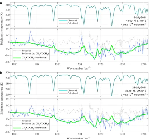
Figure 1. Examples of acetone detection in Infrared Atmospheric Sounding Interferometer spectra taken over land (a) and ocean (b). In each example, the observed and calculated spectra are displayed in the upper frame in light blue and red, respectively, while the black dotted line in the lower frame represents the fitting residuals between those (observed-calculated). The difference between the fitted spectra reconstructed with and without acetone is in solid green line, while the difference between the observed spectrum and the fitted spectrum reconstructed without acetone is in blue.
The fitted spectra (red) shown in Figure 1 match the observed spectra well, with a residual (black dotted line) mostly within the expected instrumental noise of IASI (between 0.05 and 0.2 K in the acetone range). Larger residuals occur at channels dominated by H2O and CH4absorptions and are similar in both fits, pointing toward limitations in the forward model (Atmosphit for instance does not account for CH4line mixing). The overall baseline is nonetheless reconstructed satisfactorily in the entire 1,171–1,242 cm−1range. The con-tribution of acetone can be visualized with the help of a second simulation, obtained by excluding acetone from the result of the first simulation. The residuals between the simulated spectra without acetone and the observed spectrum (blue line) or the simulated spectrum with acetone (green line) both visualize the broad
𝜈17C-C stretch band of acetone with an absorption as large as 0.4–0.5 K. Note that the retrieved columns are large (3.46 and 4.09 × 10¹⁶molec/cm2), but not unreasonably high (see section 3.2). The above analysis has been carried out on a number of spectra in different parts of the world, with similar conclusions, providing convincing evidence for the detection of acetone in IASI spectra. It also follows that—apart from observa-tions over deserts—HRI enhancements in this spectral range are indeed due to acetone. Over deserts, biases in the acetone HRI related to changes in surface type are apparent; these are removed here to a first order via a debiasing procedure (Clarisse et al., 2019; Franco et al., 2018).
2.2. NN Retrieval
Using OEM inversion for the daily global retrieval of acetone and other weak absorbers has some disad-vantages (e.g., sensitivity to retrieval parameters, forward model errors, and large computational costs; see Whitburn et al., 2016). An attractive alternative is the Artificial Neural Network for IASI (ANNI) retrieval approach, which was developed for the retrieval of NH3(Whitburn et al., 2016), and later expanded to the retrieval of a series of VOCs (Franco et al., 2018). The retrieval relies on a feedforward NN to convert the
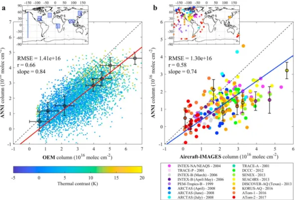
Figure 2. (a) Comparison of acetone total columns retrieved with both OEM and ANNI approaches for IASI spectra recorded on 15 July 2011 over specific regions (in inset). (b) Comparison between acetone total columns derived from composite aircraft-IMAGES profiles (located in inset), with the closest individual ANNI column obtained the same day as the composite profile. For both comparisons, the linear regression, RMSE, and coefficient of correlation (r) are given. The OEM and ANNI uncertainties are indicated for selected measurements (in black). OEM = optimal estimation method; IASI = Infrared Atmospheric Sounding Interferometer; ANNI = Artificial Neural Network for IASI; RMSE = root mean square error.
HRI into a gas total column, accounting for the state of both atmosphere and surface (e.g., emissivity, tem-perature, and H2O profiles). The implementation for acetone follows largely that of the other VOCs. We therefore refer to Franco et al. (2018) for a detailed presentation of the algorithm and only mention here the elements that are specific to acetone.
As for the other VOCs, two NNs were set up, both assuming different fixed vertical profiles of acetone repre-sentative for emission and transport regimes. These profiles were derived from the global chemistry-climate model EMAC (ECHAM5/MESSy; Jöckel et al., 2010) and are shown in Figure S1 in the supporting infor-mation. The NN performance on the training set is summarized in Figure S2. For positive thermal contrasts (i.e., the temperature difference between the surface and the air layer located just above), the performance is excellent, with a bias below 5%, and a retrieval error below 20% for columns above 1 × 10¹⁶molec/cm2 and below 50% for columns between 0.5 and 1 × 10¹⁶molec/cm2. For weakly negative thermal contrast, sen-sitivity to the lower troposphere is lost, resulting in larger errors. The actual retrieval comes with an own estimate of retrieved column uncertainty associated with each individual measurement, obtained via prop-agation of the uncertainties in the input variables. Similarly to the other VOCs, a postfilter was designed to exclude observations associated with almost no sensitivity to acetone. As explained in Franco et al. (2018), a constant, climatological background abundance (not accounted for by the HRI) needs to be added to the retrieved columns. This calibration offset was estimated here by adjusting the 2010–2015 averaged IASI-derived columns to the 2010–2015 averaged acetone columns simulated by EMAC, separately over remote land and ocean areas (see Figure S3).
3. Results
Acetone columns have been retrieved with the ANNI method from the entire IASI/Metop-A data set (Octo-ber 2007 to Novem(Octo-ber 2018) including both the morning and evening overpasses (∼9:30 a.m. and p.m., local
Geophysical Research Letters
10.1029/2019GL082052
time). The columns over land were retrieved with the NN trained with the emission gas profile, whereas those over ocean are output of the transport NN.
3.1. Column Intercomparisons
To make a first assessment of the ANNI retrieval, we present in Figure 2a a comparison with acetone retrieved with an OEM inversion from ∼10,000 IASI spectra observed over both source and remote regions (see inset of Figure 2a), following the setup described in section 2.1 and using the profiles derived from EMAC (Figure S1) as a priori. When the measurement sensitivity is low, such retrievals typically remain close to the a priori. For this reason, we limit the comparison here to the summer season, when the measure-ment sensitivity is the largest (Franco et al., 2018). The two retrievals compare favorably, with a coefficient of correlation (r) of 0.66 and a regression slope of 0.84, giving confidence in the ANNI retrieval. The rather large scatter reflects the uncertainties associated with each inversion approach and the general difficulty of retrieving acetone. Note that the estimated measurement uncertainties (black error bars) from both methods are similar (0.5–1.5 × 10¹⁶molec/cm2).
A second intercomparison has been performed with a suite of aircraft measurements (see inset in Figure 2b). For this, we built average aircraft profiles, derived from measurements taken on the same day and located no further than 150 km. Typically, the measurements range from the upper troposphere down to close to the surface. These profiles were then completed from the last available altitude by profiles from the chemistry-transport model IMAGESv2 (Müller, Stavrakou & Peeters 2018; Müller, Stavrakou, Bauwens, et al., 2018; Stavrakou et al., 2018) sampled at the time and location of the aircraft profiles and finally integrated to obtain acetone total columns. Examples of composite aircraft-IMAGES profiles and further information are provided in Figure S4. For measurements within the IASI period (after October 2007), we compared these columns directly with the closest IASI measurement obtained on the same day. For aircraft measurements before, an IASI column was constructed by averaging the observations made on the same Julian day of the available years in the October 2007 to November 2018 period. The comparison, presented in Figure 2b, gives a correlation of 0.58 and a slope of 0.74, pointing toward a possible low bias in the IASI measurements. The comparison presented here is limited by the number and type of available measure-ments (most aircraft campaigns cover only North America); a full assessment of the NN performance and acetone product will only be possible once more correlative column measurements become available. 3.2. Daily Overpasses Examples
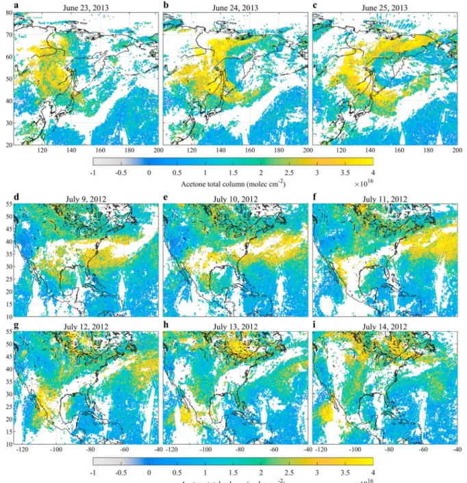
Figure 3 gives examples of acetone measurements on selected days over East Siberia (Figures 3a–3c) and North America (Figures 3d–3i) during the boreal summer. Owing to the relatively long lifetime of acetone and the ability of the NN to account for the overall lower sensitivity of IASI to the evening measurements, the a.m.- and p.m.-derived retrievals produce consistent acetone columns (Figure S5), with lowest uncertainty made in the morning over land. Therefore, both column sets have been combined to enhance the spatial coverage (they are shown separately in Figure S6). The remaining empty spaces in the acetone distributions correspond either to the gaps between successive satellite orbits, clouds, or measurements discarded by the postfilter. The distributions of the uncertainties associated with the individual retrieved columns are dis-played in Figure S7. In these examples, most column uncertainties range between 2 and 7 × 10¹⁵molec/cm2 over land, and between 4 and 9 × 10¹⁵molec/cm2over oceans where the overall weaker thermal contrast is associated with a lower sensitivity to the surface. As illustrated in Figure S8, the uncertainties are mainly driven by the HRI and of secondary importance by the thermal contrast.
These two examples highlight the dense spatial sampling achieved by IASI, and the spatial resolution of the individual measurements (pixel size of 12 km at nadir). They also illustrate at a regional scale the flex-ibility and the sensitivity of the NN-based retrievals to a fast-changing gas distribution. Indeed, Figure 3 demonstrates that IASI is able to detect background acetone levels of 0.5–1 × 10¹⁶molec/cm2over relatively remote areas like Western United States and oceans, whereas strong local enhancements of acetone column in excess of 3–4 × 10¹⁶molec/cm2are observed for instance over the boreal forests of Siberia (Figures 3a–3c) and Canada (Figures 3d–3i), as well as over Eastern and Southern United States (Figures 3d–3i), which rep-resent more than a factor of 4 increase compared to the background conditions. The retrieved columns also allow monitoring the atmospheric transport of acetone on a daily basis, as IASI detects large plumes of ace-tone that originate from these local enhancements and whose day-to-day transport can be closely tracked across both continents and oceans.
Figure 3. Acetone total columns distributions over two areas of interest (East Siberia and North America), retrieved with the Artificial Neural Network for Infrared Atmospheric Sounding Interferometer (IASI) method from individual days of IASI observations (a.m. and p.m. overpasses) , from 23 to 25 June 2013 (a–c), and from 9 to 14 July 2012 (d–i).
These regional examples highlight that the acetone column distribution is characterized by a high spa-tial and temporal heterogeneity (see also close-ups in Figure S6). Bearing in mind that the relatively long lifetime of acetone ensures an elevated background abundance of the order of 0.5–1 × 10¹⁶molec/cm2 during boreal summer,>200% enhancement can locally be observed over the continents and in concen-trated plumes (Figure 3). This is likely related to direct emissions of acetone or to strong emissions of short-lived precursors. It is worth mentioning that such heterogeneity has also been observed in sum-mertime in the Northern Hemisphere UTLS along the flight tracks of the In-service Aircraft for a Global Observing System-Civil Aircraft for the Regular Investigation of the atmosphere Based on an Instrument Container (IAGOS-CARIBIC) (e.g., Elias et al., 2011; Fischbeck et al., 2017; Sprung & Zahn, 2010).
Geophysical Research Letters
10.1029/2019GL082052
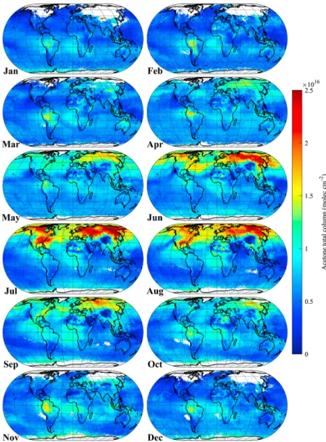
Figure 4. Monthly means (on a 0.5◦ ×0.5◦grid) of the acetone total columns retrieved with the Artificial Neural Network for Infrared Atmospheric Sounding Interferometer method from the a.m. and p.m. Infrared Atmospheric Sounding Interferometer observations over the year 2011. The white areas correspond to regions where no measurements passed the prefilters and postfilters due to clouds or poor measurement sensitivity. 3.3. Global Distribution
The global distribution of acetone and its seasonal variability as retrieved from IASI measurements are inves-tigated here through the monthly mean columns of the year 2011, averaged on a 0.5◦ ×0.5◦grid (Figure 4). Yearly averages are shown in Figure S9. The following observations can be made:
• During most of the year, there is a clear North-South gradient with more acetone in the Northern Hemi-sphere. This pattern is pronounced also in the yearly mean distributions (Figure S9) and is consistent with the currently known dominant anthropogenic and biogenic sources (primary and secondary) of acetone, which are mostly of continental origin and mainly take place in the boreal hemisphere. IASI also indicates a strong seasonal cycle in the Northern Hemisphere, with the highest acetone columns (>4 × 10¹⁶molec/cm2 in monthly mean) found in summer over land at middle and high latitudes. Nonetheless, monthly mean acetone enhancements of 1–2 × 10¹⁶molec/cm2are detected over tropical forests during the October–April period.
• Acetone concentrations in the UTLS have recently been retrieved by the Atmospheric Composition Experiment-Fourier Transform Spectrometer (ACE-FTS) in the 2004–2010 period (Dufour et al., 2016). The IASI observations confirm the spatial and seasonal patterns of acetone concentrations measured by
ACE-FTS, which also exhibit a strong latitudinal gradient and a pronounced seasonal cycle in the 30–70◦ N latitudinal band that peaks in July. Moreover, the maximum monthly mean concentrations measured by ACE-FTS are found in this month over Siberia, where IASI also detects the highest total columns (Figure 4). Another important agreement between the limb and nadir sounders is the moderate acetone burden detected within the tropics, also over tropical forests.
• These observations suggest that direct acetone emissions and/or oxidation of precursor hydrocarbons, both from the terrestrial biosphere at the Northern Hemisphere middle and high latitudes, are the main contributor to the acetone abundance and the main driver of its seasonal variability (as also shown by Jacob et al., 2002). Indeed, acetone is a by-product of plant metabolism (e.g., Fall, 1999) with light- and temperature-dependent emissions (Kirstine et al., 1998). Concomitantly, acetone is produced from the atmospheric oxidation of monoterpenes (e.g.,𝛼- and 𝛽-pinenes; Reissell et al., 1999) and methylbutenol (Goldstein & Schade, 2000) in the relative vicinity of their emission sources, as those precursors are short lived. Atmospheric degradation of anthropogenic isoalkanes, whose emissions do not show strong sea-sonal variability, may significantly contribute to acetone formation in winter when the emissions from the terrestrial vegetation are low.
• Major observable features are the continental acetone outflows over oceans, particularly strong in summer in the Northern Hemisphere. These outflows follow the dominant atmospheric circulation pattern, that is, eastward transport at middle and high latitudes, and westward transport within the tropics. Noticeable examples are the North American and Asian outflows north of 20◦N, respectively, over the Atlantic and Pacific oceans. Anthropogenic acetone precursors from the continents likely form a year-round component of those, while the strong enhancement in summer can be attributed to an increased contribution from biogenic sources.
• IASI-derived acetone is only moderately enhanced in the tropics during the fire season (October–November), unlike methanol, formic acid, or PAN retrieved with the same ANNI method (Franco et al., 2018). This likely stems from the limited emissions of both acetone and its isoalkane pre-cursors in biomass burning (Akagi et al., 2011) and argues against fires being a dominant driver of the global acetone budget.
• The background acetone abundance derived from IASI is large over remote marine areas (e.g., the Middle Pacific), with monthly mean columns regularly over 5 × 10¹⁵molec/cm2. It can be explained by long-range transport of continental precursors or, as reported by Jacob et al. (2002), by a large marine source of acetone either from the ocean or from the marine atmosphere (e.g., marine organic aerosol).
• While there is a general land-ocean continuity at middle and low latitudes, relatively sharp transitions between the columns can be observed in summer at Northern Hemisphere high latitudes. These are espe-cially apparent between the continents and the Arctic Ocean, and between Northern Canada and the Hudson Bay (Figure 4). The same discontinuities were also observed with other OVOCs (Franco et al., 2018). From a theoretical viewpoint, there is no reason for this to happen, as the NNs are perfectly capa-ble of taking into account large differences in surface temperature. The likely reason for these are biases in the underlying input data, for instance on the surface or atmospheric temperature, or the fact that the assumed vertical profiles differ greatly from the true profiles. This is one aspect of the work that needs improvement in the future.
4. Conclusions
In this work, we have demonstrated that acetone can be measured from IASI spectra and that its total column can be retrieved globally and on a daily basis using a NN-based retrieval approach. Despite many advantages, the ANNI retrievals introduced have some drawbacks discussed in detail by Franco et al. (2018), Van Damme et al. (2017), and Whitburn et al. (2016). In particular, the use of fixed gas profiles for the NN training shows clear limitations in some remote environments, like the polar and ice-covered regions. The implementation of a fully parameterized gas vertical profile for the NN training, and an improved correction of the emissivity issues over deserts, are part of further developments that would enhance the retrieval.
The ANNI-acetone product, which consists of over 10 years of daily global distributions of gas total column from IASI/Metop-A, has been obtained from a single sounder and therefore can be regarded as a long-term record suitable for investigating the atmospheric abundance, transport, variability, and long-term evolu-tion of acetone throughout the global troposphere. With IASI/Metop-B and -C (launched in 2012 and 2018, respectively), and the three future IASI-NG (New Generation), the time series can be extended to ∼40 years. The ANNI-acetone product also has the potential to fill gaps in the current uncertainties on the atmospheric acetone budget by providing global constraints to modeled source and sink processes.
Geophysical Research Letters
10.1029/2019GL082052
The acetone retrievals presented here add to the existing global IASI products (e.g., methanol, formic acid, and PAN). Altogether, this unique satellite data set provides an extensive view of major atmospheric OVOCs and an improved understanding of their impact on tropospheric chemistry.
References
Akagi, S. K., Yokelson, R. J., Wiedinmyer, C., Alvarado, M. J., Reid, J. S., Karl, T., & Wennberg, P. O. (2011). Emission factors for open and domestic biomass burning for use in atmospheric models. Atmospheric Chemistry and Physics, 11(9), 4039–4072. https://doi.org/10.5194/acp-11-4039-2011
Arnold, S. R., Chipperfield, M. P., & Blitz, M. A. (2005). A three-dimensional model study of the effect of new temperature-dependent quantum yields for acetone photolysis. Journal of Geophysical Research, 110, D22305. https://doi.org/10.1029/2005JD005998 Brewer, J. F., Bishop, M., Kelp, M., Keller, C. A., Ravishankara, A. R., & Fischer, E. V. (2017). A sensitivity analysis of
key natural factors in the modeled global acetone budget. Journal of Geophysical Research: Atmospheres, 122, 2043–2058. https://doi.org/10.1002/2016JD025935
Brühl, C., Pöschl, U., Crutzen, P. J., & Steil, B. (2000). Acetone and PAN in the upper troposphere: Impact on ozone production from aircraft emissions. Atmospheric Environment, 34(23), 3931–3938. https://doi.org/10.1016/s1352-2310(00)00159-x
Clarisse, L., Clerbaux, C., Franco, B., Hadji-Lazaro, J., Whitburn, S., Kopp, A. K., & Coheur, P. F. (2019). A decadal data set of global atmospheric dust retrieved from IASI satellite measurements. Journal of Geophysical Research: Atmospheres, 124, 1618–1647. https://doi.org/10.1029/2018JD029701
Clarisse, L., Coheur, P. F., Prata, F., Hadji-Lazaro, J., Hurtmans, D., & Clerbaux, C. (2013). A unified approach to infrared aerosol remote sensing and type specification. Atmospheric Chemistry and Physics, 13(4), 2195–2221. https://doi.org/10.5194/acp-13-2195-2013 Clarisse, L., R'Honi, Y., Coheur, P. F., Hurtmans, D., & Clerbaux, C. (2011). Thermal infrared nadir observations of 24 atmospheric gases.
Geophysical Research Letters, 38, L10802. https://doi.org/10.1029/2011GL047271
Clerbaux, C., Boynard, A., Clarisse, L., George, M., Hadji-Lazaro, J., Herbin, H., & Coheur, P. F. (2009). Monitoring of atmospheric composition using the thermal infrared IASI/MetOp sounder. Atmospheric Chemistry and Physics, 9(16), 6041–6054. https://doi.org/ 10.5194/acp-9-6041-2009
Coheur, P. F., Barret, B., Turquety, S., Hurtmans, D., Hadji-Lazaro, J., & Clerbaux, C. (2005). Retrieval and characterization of ozone vertical profiles from a thermal infrared nadir sounder. Journal of Geophysical Research, 110, D24303. https://doi.org/10.1029/2005JD005845 Coheur, P. F., Clarisse, L., Turquety, S., Hurtmans, D., & Clerbaux, C. (2009). IASI measurements of reactive trace species in biomass
burning plumes. Atmospheric Chemistry and Physics, 9(15), 5655–5667. https://doi.org/10.5194/acp-9-5655-2009
Coheur, P. F., Herbin, H., Clerbaux, C., Hurtmans, D., Wespes, C., Carleer, M., & Bernath, P. F. (2007). ACE-FTS observation of a young biomass burning plume: First reported measurements of C2H4, C3H6O, H2CO and PAN by infrared occultation from space. Atmospheric Chemistry and Physics, 7(20), 5437–5446. https://doi.org/10.5194/acp-7-5437-2007
Dufour, G., Szopa, S., Harrison, J. J., Boone, C. D., & Bernath, P. F. (2016). Seasonal variations of acetone in the upper troposphere–lower stratosphere of the northern midlatitudes as observed by ACE-FTS. Journal of Molecular Spectroscopy, 323, 67–77. https://doi.org/10.1016/j.jms.2016.02.006
Elias, T., Szopa, S., Zahn, A., Schuck, T., Brenninkmeijer, C., Sprung, D., & Slemr, F. (2011). Acetone variability in the upper troposphere: Analysis of CARIBIC observations and LMDz-INCA chemistry-climate model simulations. Atmospheric Chemistry and Physics, 11(15), 8053–8074. https://doi.org/10.5194/acp-11-8053-2011
Fall, R. (1999). Biogenic emissions of volatile organic compounds from higher plants. In Reactive Hydrocarbons in the Atmosphere (pp. 41–96). San Diego, CA: Elsevier. https://doi.org/10.1016/b978-012346240-4/50003-5
Fischbeck, G., Bönisch, H., Neumaier, M., Brenninkmeijer, C. A. M., Orphal, J., Brito, J., & Zahn, A. (2017). Acetone-CO enhancement ratios in the upper troposphere based on 7 years of CARIBIC data: New insights and estimates of regional acetone fluxes. Atmospheric Chemistry and Physics, 17(3), 1985–2008. https://doi.org/10.5194/acp-17-1985-2017
Fischer, E. V., Jacob, D. J., Millet, D. B., Yantosca, R. M., & Mao, J. (2012). The role of the ocean in the global atmospheric budget of acetone. Geophysical Research Letters, 39, L01807. https://doi.org/10.1029/2011GL050086
Fischer, E. V., Jacob, D. J., Yantosca, R. M., Sulprizio, M. P., Millet, D. B., Mao, J., & Deolal, S. P. (2014). Atmospheric peroxyacetyl nitrate (PAN): A global budget and source attribution. Atmospheric Chemistry and Physics, 14(5), 2679–2698. https://doi.org/10.5194/ acp-14-2679-2014
Folberth, G. A., Hauglustaine, D. A., Lathière, J., & Brocheton, F. (2006). Interactive chemistry in the Laboratoire de Météorologie Dynamique general circulation model: Model description and impact analysis of biogenic hydrocarbons on tropospheric chemistry. Atmospheric Chemistry and Physics, 6(8), 2273–2319. https://doi.org/10.5194/acp-6-2273-2006
Folkins, I., & Chatfield, R. (2000). Impact of acetone on ozone production and OH in the upper troposphere at high NOx. Journal of Geophysical Research, 105(D9), 11,585–11,599. https://doi.org/10.1029/2000JD900067
Franco, B., Clarisse, L., Stavrakou, T., Müller, J. F., Van Damme, M., Whitburn, S., & Coheur, P. F. (2018). A general framework for global retrievals of trace gases from IASI: Application to methanol, formic acid, and PAN. Journal of Geophysical Research: Atmospheres, 123, 13,963–13,984. https://doi.org/10.1029/2018JD029633
Goldstein, A. H., & Schade, G. W. (2000). Quantifying biogenic and anthropogenic contributions to acetone mixing ratios in a rural environment. Atmospheric Environment, 34(29–30), 4997–5006. https://doi.org/10.1016/s1352-2310(00)00321-6
Gordon, I. E., Rothman, L. S., Hill, C., Kochanov, R. V., Tan, Y., Bernath, P. F., & Zak, E. J. (2017). The HITRAN 2016 molecular spectroscopic database. Journal of Quantitative Spectroscopy and Radiative Transfer, 203, 3–69. https://doi.org/10.1016/j.jqsrt.2017.06.038
Harrison, J. J., Humpage, N., Allen, N. D. C., Waterfall, A. M., Bernath, P. F., & Remedios, J. J. (2011). Mid-infrared absorption cross sections for acetone (propanone). Journal of Quantitative Spectroscopy and Radiative Transfer, 112(3), 457–464. https://doi.org/10.1016/ j.jqsrt.2010.09.002
Jacob, D. J., Field, B. D., Jin, E. M., Bey, I., Li, Q., Logan, J. A., & Singh, H. B. (2002). Atmospheric budget of acetone. Journal of Geophysical Research, 107(D10), 4100. https://doi.org/10.1029/2001JD000694
Jaeglé, L., Jacob, D. J., Brune, W. H., & Wennberg, P. O. (2001). Chemistry of HOx radicals in the upper troposphere. Atmospheric Environment, 35(3), 469–489. https://doi.org/10.1016/s1352-2310(00)00376-9
Jöckel, P., Kerkweg, A., Pozzer, A., Sander, R., Tost, H., Riede, H., & Kern, B. (2010). Development cycle 2 of the Modular Earth Submodel System (MESSy2). Geoscientific Model Development, 3(2), 717–752. https://doi.org/10.5194/gmd-3-717-2010
Acknowledgments
The research has been supported by the project OCTAVE (Oxygenated Compounds in the Tropical Atmosphere: Variability and Exchanges (http://octave.
aeronomie.be) of the Belgian Research Action through Interdisciplinary Networks(BRAIN-be; 2017–2021; Research project BR/175/A2/OCTAVE) and by the IASI.Flow Prodex arrangement (ESA-BELSPO). L. Clarisse is a research associate supported by the F.R.S.-FNRS. The French scientists are grateful to CNES and Centre National de la Recherche Scientifique (CNRS) for financial support. IASI is a joint mission of Eumetsat and the Centre National d'Etudes Spatiales (CNES, France). The IASI Level-1C data are distributed in near real time by Eumetsat through the EumetCast system distribution. The authors acknowledge the Aeris data infrastructure
(https://www.aeris-data.fr/) for providing access to the IASI Level-1C data and Level-2 temperature data. We would very much like to thank all the people involved in the aircraft campaigns and for making the data publicly available. The data were downloaded from the https://esrl.noaa.gov/ csd/projects/senex/ (SENEX), https://espoarchive.nasa.gov/archive (ATom), and https://www-air.larc. nasa.gov/missions/merges/ (all other campaigns). The IASI acetone data presented in this paper are publicly available on the AERIS repository (https://iasi.aeris-data.fr/C3H6O).
Khan, M. A. H., Cooke, M. C., Utembe, S. R., Archibald, A. T., Maxwell, P., Morris, W. C., & Shallcross, D. E. (2015). A study of global atmospheric budget and distribution of acetone using global atmospheric model STOCHEM-CRI. Atmospheric Environment, 112, 269–277. https://doi.org/10.1016/j.atmosenv.2015.04.056
Kirstine, W., Galbally, I., Ye, Y., & Hooper, M. (1998). Emissions of volatile organic compounds (primarily oxygenated species) from pasture. Journal of Geophysical Research, 103(D9), 10,605–10,619. https://doi.org/10.1029/97JD03753
Lewis, A. C., Hopkins, J. R., Carpenter, L. J., Stanton, J., Read, K. A., & Pilling, M. J. (2005). Sources and sinks of acetone, methanol, and acetaldehyde in North Atlantic marine air. Atmospheric Chemistry and Physics, 5(7), 1963–1974. https://doi.org/10.5194/acp-5-1963-2005 Marandino, C. A., Bruyn, W. J. D., Miller, S. D., Prather, M. J., & Saltzman, E. S. (2005). Oceanic uptake and the global atmospheric acetone
budget. Geophysical Research Letters, 32, L15806. https://doi.org/10.1029/2005GL023285
McKeen, S. A., Gierczak, T., Burkholder, J. B., Wennberg, P. O., Hanisco, T. F., Keim, E. R., & Fahey, D. W. (1997). The photochemistry of acetone in the upper troposphere: A source of odd-hydrogen radicals. Geophysical Research Letters, 24(24), 3177–3180. https://doi.org/10.1029/97GL03349
Moore, D. P., Remedios, J. J., & Waterfall, A. M. (2012). Global distributions of acetone in the upper troposphere from MIPAS spectra. Atmospheric Chemistry and Physics, 12(2), 757–768. https://doi.org/10.5194/acp-12-757-2012
Müller, J. F., & Brasseur, G. (1999). Sources of upper tropospheric HOx: A three-dimensional study. Journal of Geophysical Research, 104(D1), 1705–1715. https://doi.org/10.1029/1998JD100005
Müller, J. F., Stavrakou, T., Bauwens, M., Compernolle, S., & Peeters, J. (2018). Chemistry and deposition in the Model of Atmospheric composition at Global and Regional scales using Inversion Techniques for Trace gas Emissions (MAGRITTE v1.0). Part B. Dry deposition. Geoscientific Model Development Discussions, 1–49. https://doi.org/10.5194/gmd-2018-317
Müller, J. F., Stavrakou, T., & Peeters, J. (2018). Chemistry and deposition in the Model of Atmospheric composition at Global and Regional scales using Inversion Techniques for Trace gas Emissions (MAGRITTEv1.0). Part A. Chemical mechanism. Geoscientific Model Development Discussions, 1–59. https://doi.org/10.5194/gmd-2018-316
Potter, C., Klooster, S., Bubenheim, D., Singh, H. B., & Myneni, R. (2003). Modeling terrestrial biogenic sources of oxygenated organic emissions. Earth Interactions, 7(7), 1–15. https://doi.org/10.1175/1087-3562(2003)007<0001:mtbsoo>2.0.co;2
Pozzer, A., Pollmann, J., Taraborrelli, D., Jöckel, P., Helmig, D., Tans, P., & Lelieveld, J. (2010). Observed and simulated global distribution and budget of atmospheric C2-C5alkanes. Atmospheric Chemistry and Physics, 10(9), 4403–4422. https://doi.org/10.5194/ acp-10-4403-2010
Read, K. A., Carpenter, L. J., Arnold, S. R., Beale, R., Nightingale, P. D., Hopkins, J. R., & Pickering, S. J. (2012). Multiannual observations of acetone, methanol, and acetaldehyde in remote tropical Atlantic air: Implications for atmospheric OVOC budgets and oxidative capacity. Environmental Science & Technology, 46(20), 11,028–11,039. https://doi.org/10.1021/es302082p
Reissell, A., Harry, C., Aschmann, S. M., Atkinson, R., & Arey, J. (1999). Formation of acetone from the OH radical- and O3-initiated
reactions of a series of monoterpenes. Journal of Geophysical Research, 104(D11), 13,869–13,879. https://doi.org/10.1029/1999jd900198 Remedios, J. J., Allen, G., Waterfall, A. M., Oelhaf, H., Kleinert, A., & Moore, D. P. (2007). Detection of organic compound signatures in infra-red, limb emission spectra observed by the MIPAS-B2 balloon instrument. Atmospheric Chemistry and Physics, 7(6), 1599–1613. https://doi.org/10.5194/acp-7-1599-2007
Rodgers, C. D. (2000). Inverse methods for atmospheric sounding. WORLD SCIENTIFIC https://doi.org/10.1142/3171
Safieddine, S. A., Heald, C. L., & Henderson, B. H. (2017). The global nonmethane reactive organic carbon budget: A modeling perspective. Geophysical Research Letters, 44, 3897–3906. https://doi.org/10.1002/2017GL072602
Seinfeld, J. H., & Pandis, S. N. (2016). Atmospheric chemistry and physics: From air pollution to climate change. New York: Wiley. Retrieved from https://www.ebook.de/de/product/25599491/john h seinfeld spyros n pandis_atmospheric chemistry and physics.html. Singh, H. B., Chen, Y., Staudt, A., Jacob, D., Blake, D., Heikes, B., & Snow, J. (2001). Evidence from the Pacific troposphere for large global
sources of oxygenated organic compounds. Nature, 410(6832), 1078–1081. https://doi.org/10.1038/35074067
Singh, H. B., Kanakidou, M., Crutzen, P. J., & Jacob, D. J. (1995). High concentrations and photochemical fate of oxygenated hydrocarbons in the global troposphere. Nature, 378(6552), 50–54. https://doi.org/10.1038/378050a0
Singh, H. B., O'Hara, D., Herlth, D., Sachse, W., Blake, D. R., Bradshaw, J. D., & Crutzen, P. J. (1994). Acetone in the atmosphere: Distribution, sources, and sinks. Journal of Geophysical Research, 99(D1), 1805–1819. https://doi.org/10.1029/93JD00764
Sinha, V., Williams, J., Meyerhöfer, M., Riebesell, U., Paulino, A. I., & Larsen, A. (2007). Air-sea fluxes of methanol, acetone, acetaldehyde, isoprene and DMS from a Norwegian fjord following a phytoplankton bloom in a mesocosm experiment. Atmospheric Chemistry and Physics, 7(3), 739–755. https://doi.org/10.5194/acp-7-739-2007
Sprung, D., & Zahn, A. (2010). Acetone in the upper troposphere/lowermost stratosphere measured by the CARIBIC passenger aircraft: Distribution, seasonal cycle, and variability. Journal of Geophysical Research, 115, D16301. https://doi.org/10.1029/2009JD012099 Stavrakou, T., Müller, J. F., Bauwens, M., Smedt, I. D., Roozendael, M. V., & Guenther, A. (2018). Impact of short-term climate variability
on volatile organic compounds emissions assessed using OMI satellite formaldehyde observations. Geophysical Research Letters, 45, 8681–8689. https://doi.org/10.1029/2018GL078676
Taddei, S., Toscano, P., Gioli, B., Matese, A., Miglietta, F., Vaccari, F. P., & Williams, J. (2009). Carbon dioxide and acetone air-sea fluxes over the Southern Atlantic. Environmental Science & Technology, 43(14), 5218–5222. https://doi.org/10.1021/es8032617
Van Damme, M., Whitburn, S., Clarisse, L., Clerbaux, C., Hurtmans, D., & Coheur, P. F. (2017). Version 2 of the IASI NH3 neural network retrieval algorithm: Near-real-time and reanalysed datasets. Atmospheric Measurement Techniques, 10(12), 4905–4914. https://doi.org/10.5194/amt-10-4905-2017
Walker, J. C., Dudhia, A., & Carboni, E. (2011). An effective method for the detection of trace species demonstrated using the MetOp Infrared Atmospheric Sounding Interferometer. Atmospheric Measurement Techniques, 4(8), 1567–1580. https://doi.org/10.5194/amt-4-1567-2011
Wennberg, P. O., Hanisco, T. F., Jaeglé, L., Jacob, D. J., Hintsa, E. J., Lanzendorf, E. J., & Bui, T. P. (1998). Hydrogen radicals, nitrogen radicals, and the production of O3in the upper troposphere. Science, 279(5347), 49–53. https://doi.org/10.1126/science.279.5347.49
Whitburn, S., Damme, M. V., Clarisse, L., Bauduin, S., Heald, C. L., Hadji-Lazaro, J., & Coheur, P. F. (2016). A flexible and robust neural network IASI-NH3retrieval algorithm. Journal of Geophysical Research: Atmospheres, 121, 6581–6599. https://doi.org/10.1002/ 2016JD024828
Williams, J., Holzinger, R., Gros, V., Xu, X., Atlas, E., & Wallace, D. W. R. (2004). Measurements of organic species in air and seawater from the tropical Atlantic. Geophysical Research Letters, 31, L23S06. https://doi.org/10.1029/2004GL020012