Drag optimization for the nose of a vehicle moving through a channel guideway

Drag Optimization for the Nose of a Vehicle

Moving Through a Channel Guideway

by

Robert Craig Castellino

B.S., Mechanical Engineering Duke University

(1991)

Submitted to the Department of

Aeronautics and Astronautics in Partial Fulfillment of the Requirements for the

Degree of

MASTER OF SCIENCE in Aeronautics and Astronautics

at the

Massachusetts Institute of Technology

May 1993

© Robert Craig Castellino, 1993. All rights reserved

Signature of I

Depamentf Aeronautics and Astronautics May, 1993

Approved by

Dr. Timothy M. Barrows Technical Supervisor, Drapet Laboratory

,( /

Certified by

Professor Marten T. Landahl

Department of Aeronautics and Astronautics Thesis Supervisor

\ ofessor Harold Y. Wachman 'Chfii;,Dbpartmental Griduate Committee Department of Aeronautics and Astronautics Accepted by.

Aero

[JUN 08

1993

Drag Optimization for the Nose of a Vehicle

Moving Through a Channel Guideway

by

Robert Craig Castellino

Submitted to the Department of Aeronautics and Astronautics on May 7, 1993 in partial fulfillment of the

requirements for the degree of Master of Science

Abstract

A model is first developed to simulate vortex shedding, due to the motion of the nose of a vehicle through a channel guideway, using slender body theory and the concept of mirror images. This model consists of an expanding cylinder between two parallel guidewalls. It is incorporated first into an analytical approach to the calculation of drag. A numerical approach is attempted next because of the failure of the analytical approach. The first numerical problem simulates the flow over a circular cylinder in a free stream. The second problem simulates vortex shedding behind a flat plate in a free stream. The numerical schemes used to solve the first two problems are now incorporated into a third scheme which simulates vortex shedding due to the movement of a vehicle nose through a channel guideway. The energy in the shed vortices is related to drag, and drag is manipulated to find an optimum vehicle nose length.

Technical Supervisor:

Thesis Supervisor:

Timothy M. Barrows

Group Leader, Dynamical Systems Division The Charles Stark Draper Laboratory, Inc. Dr. Marten T. Landahl

Acknowledgements

I would like to begin by thanking the Charles Stark Draper Laboratory for giving me the opportunity to pursue my dream of attending graduate school at MIT. The pleasant atmosphere and generous financial support have helped to make the past two years very memorable for me. I would especially like to express my gratitude to my thesis supervisor Tim Barrows. First of all, he has written sections 1.1 through 1.3 in this report. He has greatly enriched my knowledge of fluid dynamics and has always pointed me in the right direction when problems arose with my research. I would also like to thank Prof. Shiela Widnall who invited me to attend MIT and who has served as my thesis supervisor at MIT for the majority of the last two years. Thank you Prof. Marten Landahl for agreeing to take over as my thesis supervisor when Prof. Widnall could no longer perform that duty.

Thanks go next to everyone in Matthews, especially to my parents who have in the past and who continue to support my career decisions. I am really looking forward to spending more time with you next year. Maybe we can even go to the beach together again. Thanks also to Sharon Castellino and Renato Santos for your support. I am so glad that Sharon and I could live together this year. I am sorry that I have to leave, but you will be in my thoughts next year; I will try to stay closer to you in the future. Now, as for all those French guys who deserted me, I miss all of you. I am so glad that I was able to meet you Christophe and Pierre. We really had a lot of fun together. I hope I didn't annoy you too much by watching Duke basketball, Christophe. And I hope I was a good English teacher, Pierre. I would like to thank Coach Candace Royer and the MIT womens' tennis team. You have brought more happiness and joy into my life, just by your presence and concern about me, than you could ever know. Congrats and good luck to all of you at nationals. Last, but not least, thank you Carol for coming into my life. Your presence has always been a source of great happiness for me. I could not imagine being as happy at MIT if it had not been for you. I just want you to know that I care about you a great deal and I will always be here for you, my little girl in the yellow coat.

ACKNOWLEDGEMENT

This thesis was prepared at The Charles Stark Draper Laboratory, Inc., under Contract DTFR53-91-C-00072

Publication of this thesis does not constitute approval by Draper or the sponsoring agency of the findings or conclusions contained herein. It is published for the exchange and stimulation of ideas.

I hereby assign my copyright of this thesis to The Charles Stark Draper Laboratory, Inc., Cambridge, Massachusetts.

I

,3

Permission is hereby granted by The Charles Stark Draper Laboratory, Inc., to the Massachusetts Institute of Technology to reproduce any or all of this thesis.

Contents

1 Introduction

1.1 Foundation for Drag Optimization Studies 3

1.2 Application of Inviscid Flow Theory 4

1.3 The Role of Viscosity in Estimating Front-End Drag 5

1.4 Solution Methods for Estimating Front-End Drag 6 2 Strategies for Modeling of Flow Problems

2.1 Construction of Models for Fluid Flow Problems 9 2.2 Analytical Approach to Front-End Vortex Drag 12

2.3 Numerical Approach to Front-End Vortex Drag 16

3 Simulation od Flow over a Circular Cylinder

3.1 Modeling of Flow over a Circular Cylinder 18

3.2 Localized Analytical Correction of Numerical Result 19 3.3 Comparison of Analytical and Corrected Numerical Solutions 21 4 Simulation of Vortex Shedding behind a Flat Plate

4.1 Modeling of Vortex Shedding behind a Flat Plate 23 4.2 Numerical Vortex Shedding Results and Problems 25 4.3 Energy in Vorticity Shed behind a Flat Plate 26

5 Simulation of Vortex Shedding from a Channel Guideway

5.1 Modeling of Vortex Shedding with an Expanding Cylinder 33

5.2 Modeling of Vortex Shedding with a Growing Source 36

5.3 Results of Vortex Shedding with a Growing Source 38

5.4 Calculation of Kinetic Energy due to Bow Vortices 40

5.5 Relation of Kinetic Energy to Total Nose Drag 43

5.6 Optimization of Vehicle Nose Length based on Total Nose Drag 45

6 Conclusions ₄₇

Chapter 1

Introduction

1.1 Foundation for Drag Optimization Studies

In the 1960's the Office of High Speed Ground Transportation sponsored a study by Tracked Hovercraft Limited [16] to conduct wind tunnel tests of three guideway configurations:

1. The inverted T 2. The channel 3. The box beam

This study showed that the channel guideway had more drag than either of the other configurations. However, the researchers who conducted this study did not have any systematic method for selecting the vehicle configurations which were used in these tests. The result was that the vehicle shapes were chosen rather arbitrarily. It is quite possible that different vehicle shapes would have resulted in different results. It appears that no one asked the simple question "Why is the drag of the channel configuration greater than that of the others?". Since drag is associated with flow over the surface of the vehicle and the channel vehicle had less surface than either the inverted T or the box beam vehicle, one might have expected the opposite result. This question will be answered in the discussion which follows.

The channel guideway offers certain advantages, and in fact researchers at the Japanese National Railroad (JNR) have selected this configuration for their maglev vehicle. Thus an understanding of the fundamental reason for this extra drag would be very useful, especially if it provided insight into ways to reduce this effect. If the drag difference could be narrowed, designers could feel free to choose the channel guideway configuration without incurring a burdensome energy penalty.

It appears that the Japanese and all previous designers of high speed channel guideway vehicles have not thought about the fundamentals of the flow in the front region. The result is that the front end of these vehicles all have conventional streamlining, i.e. they end up looking like the nose of a subsonic passenger airliner.

1.2 Application of Inviscid Flow Theory

The speed regime in which a maglev vehicle would operate can be described using incompressible aerodynamics. That is, flow speeds relative to the vehicle body are not expected to approach the speed of sound, with the result that the air density can be considered to be constant. Another important simplification is to assume that the effects of viscosity can be neglected. If this assumption is valid we have what is known as inviscid flow. If the flow is truly inviscid, there can be no aerodynamic drag. In fact, Kelvin's Theorem states that in steady inviscid flow no aerodynamic forces of any kind can be generated. Pressures can be produced on the body, but they act in such a way as to produce no net force. Thus, it might seem that nothing could be learned about aerodynamic forces from inviscid flow theory. One of the great breakthroughs in aerodynamics was the realization that if we have two-dimensional flow over an airfoil with a sharp trailing edge, the effect of viscosity will produce a net circulation such that the streams above and below the airfoil flow smoothly off the trailing edge. This is known as the Kutta condition. The lift is directly proportional to this circulation. The important point is that a method was developed to compute the lift on an airfoil without going into the details of the boundary layer. More advanced theories were able to compute the induced drag, or drag due to lift, associated with the three-dimensional flow over a wing, while still avoiding direct computation of the effects of viscosity. The research reported herein accomplishes a similar result; namely, inviscid flow theory has been used to compute an important component of the drag. The remainder of the drag would best be determined empirically.

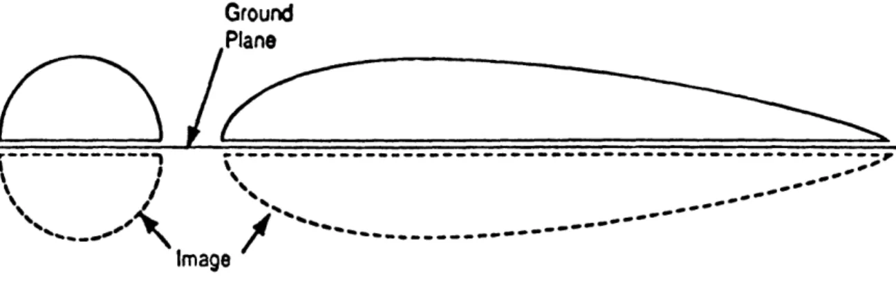
For inviscid flow, an easy way to represent the flow around an object traveling near a ground plane is to imagine that there is a mirror image of the object below the ground plane, and both objects are traveling through unrestricted air. The resulting symmetry means that there is no flow across the ground plane, as required. In this situation, one can obtain good streamlining if the object plus its image form a shape which would be well-streamlined in the absence of the ground plane. In other words, take a conventional streamlined body like an airplane fuselage and cut it in half to form a good shape for operation near a ground plane, as shown in Fig. 1.1. This line of thinking is apparently what has motivated maglev researchers at the JNR, judging by the design shown in Fig. 1.2. It represents the state of the art for this particular niche of aerodynamics, which apparently has not advanced in the last 15 years, in either the U.S. or Japan. To summarize, the effect of the horizontal plane of the channel is taken into account, but no recognition is given to the presence of the guidewalls.

Ground Plane

---- --- --- --- --- --- ---- --- --- m

---Image

Figure 1.1. A body plus its mirror image can be used to represent a ground Plane

1 6.400 21.600

Figure 1.2. The JNR maglev Vehicle

1.3 The Role of Viscosity in Estimating Front-End Drag

When viscosity is introduced, the image method is only partially valid. This method only produces a condition of zero flow across the plane of symmetry, it does nothing to establish the true condition of viscous flow which requires that the velocity be zero both normal and tangential to the ground. Let us divide the flow in Fig. 1.1 into the "outer" flow which goes over the vehicle and the "channel" flow between the vehicle and the ground plane. In the outer region it is valid to assume that the flow is basically the same as inviscid flow plus a thin boundary layer on the surface, so that the outer flow will be well-represented by the image method. However, the channel flow will show some differences from the real situation in which the vehicle travels over the ground, because of the presence of the ground boundary layer. If the height of the channel is comparable to the boundary layer thickness, the channel flow will be quite different. Let us pursue the simple flow situation shown in Fig. 1.1. In this figure the outer flow is radially outward near the front of the vehicle and radially inward near the back. If sidewalls are added,

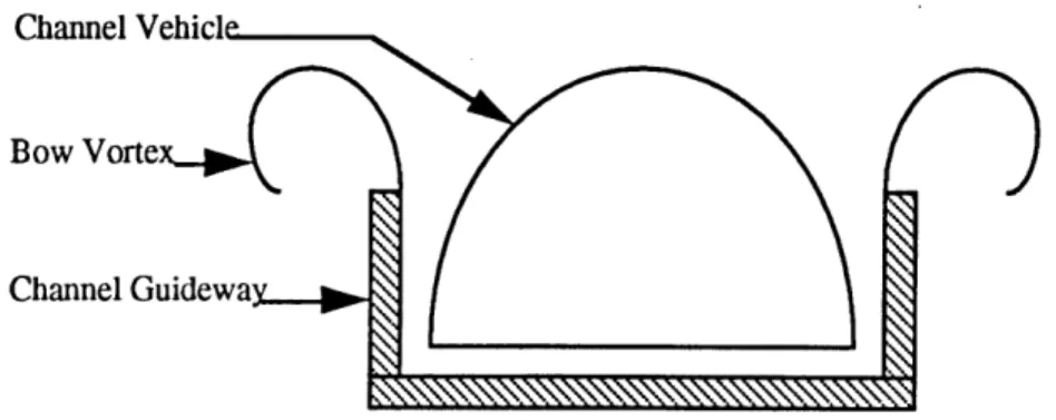
we obtain the flow situation shown in Fig. 1.3. We can easily perceive that the flow will not be able to go around the sharp turns at the top of the guidewalls, in other words the flow on each guidewall will separate and form a "bow vortex". These vortices contain energy, and all this energy is directly related to the front-end drag. This is the answer to the question posed at the beginning of this chapter. The drag of a vehicle in a channel is greater than that of a vehicle in an inverted T guideway because of these vortices.

Channel Vehicle

Bow Vorte

Channel Guidewa

Figure 1.3. Cross-Section of Vortex Shedding in a Channel Guideway

An important point is that the strength of the bow vortices can be calculated from slender body theory [2]. This is in contrast to the drag due to the boundary layer on the surface of the vehicle, which is so hard to calculate that researchers universally resort to wind tunnel measurements if an accurate value is required. It is this empirical nature of the subject of drag which has caused previous researchers to overlook the fact that for the front-end problem, a valuable theoretical advance is still possible without going into the details of the boundary layer. The separation of the flow off the top edges of the guidewalls is analogous to the Kutta condition for an airfoil. In both cases, the fact that the flow cannot be expected to turn around a sharp corner is used in conjunction with inviscid aerodynamic theory to produce a relatively simple result. The crucial advantage of using the relatively simple inviscid theory is that the relationship between the vehicle shape and the front-end drag can be established, and an optimized nose shape can be derived.

1.4 Solution Methods for Estimating Front-End Drag

First, a mathematical model must be conceived to simulate the shedding of bow vortices off the tips of the channel guideway. The construction of this model takes advantage of slender body theory and the concept of mirror images, see Fig. 1.1, in order to facilitate the calculation of drag. The simulation begins by initially fixing a slab of fluid at an arbitrary location in the channel guideway. The front-end, or nose, of a vehicle, such as the one in Fig. 1.2, is then allowed to penetrate the fluid slab in successive cross-sections. As each nose cross-section passes through

the fluid slab, additional vorticity is shed off the tips of the channel guidewalls. The shed vorticity, as discussed above in section 1.3, is the major source of energy in each fluid slab. And, it is this energy that is translated into front-end drag of a channel vehicle.

The geometrical model for this phenomenon, which employs the image technique discussed in section 1.2, consists of a cylinder, or its singular equivalent, a point source, which grows gradually in circumference between two parallel walls of finite length. Each incremental increase in the circumference of the cylinder corresponds to deeper penetration by the nose of the fluid slab and to a change in the nose cross-section seen by the stationary fluid slab. It is important to notice that only the upper half or the lower half of this model simulates the real flow problem. However, this model uses the image technique because it facilitates the calculation of drag by avoiding the complicated flow beneath the vehicle. As the cylinder grows in circumference it fills the space between the walls and pushes fluid out.

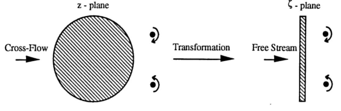
The energy in the bow vortices can either be calculated analytically or numerically. However, since an analytical solution to a fluid flow problem is always considered more valuable because of its mathematical rigor and is often used to check a more complicated numerical solution, it is attempted first. The problem for which an analytical solution is sought is that of mapping the vortices shed behind a cylinder in the presence of a cross-flow to analogous locations behind a flat plate in an oncoming free stream.

z - plane - plane

Cross-Flow Transformation Free Stream

Figure 1.4. Transformation of Vortex Positions

Milne-Thomson has mathematically demonstrated the existence of so-called "magic points" behind a cylinder in a cross-flow. That is, he has been able to prove the existence of stable locations for vortices shed off a circular cylinder in a cross-flow [13]. The objective of this analytical investigation is to locate analogous stable positions for vortices shed behind a flat plate in a free stream. If these positions do exist such that they map to magic points juxtaposed to a cylinder in a cross-flow, computation of energy in the real flow due to the existence of shed bow vortices is much simpler. This is because Milne-Thomson has derived an analytical expression

for the strengths of vortices sitting at magic points behind a cylinder in a cross-flow [13]. These vortex strengths may in turn be directly related to energy and then to drag in the mapped problem of a flat plate with shed vorticity.

An alternative approach is to use numerical algorithms to compute the energy in the bow vortices. These algorithms are based on techniques from slender body theory and use panel methods which employ discrete point singularities in an inviscid, incompressible flow [1]. The geometrical model is constructed using point vortices to form the shape of the vehicle cross-section and the walls of the channel guideway while a point source is used to simulate growth as the nose incrementally penetrates a fluid slab in the guideway. In order to establish the validity of the method, two simpler and more elementary problems must first be attacked with the numerical method: 1. the problem of the flow about a circular cylinder in a free stream and 2. the problem of vortex shedding off a flat plate oriented perpendicular to a free stream. The results from each of these simulations can easily be verified using the corresponding well-known analytical solutions. The numerical algorithms used for each of these problems may then be superimposed to solve the larger problem of vortex shedding due to the existence of an expanding cylinder, simulated with a point source of known strength, between two parallel walls. Recall that only the upper or lower half of this model corresponds to the physics of the real flow. It is this final model that provides an estimate for the vortex drag of a vehicle which moves in a channel guideway and this eventually leads to the calculation of an optimum nose length.

Chapter 2

Strategies for Modeling of Flow Problems

2.1 Construction of Models for Fluid Flow Problems

In the field of fluid dynamics, because many systems ranging from aircraft to hydo-electric dams are too large and expensive to build solely for the purpose of engineering analysis, they are usually analyzed using scaled-down models. When those models are mathematical in nature, theoretical fluid dynamicists must have tools to construct their models. The tools of the theoretical fluid dynamicist are singularities, also referred to as elementary flows. Used in analytical as well as in some numerical solutions, elementary flows are used to duplicate the geometry of many problems in fluids. Multiple elementary flows when positioned appropriately are used, for example, to represent the wing of an airplane or the wake behind the wing. In the analyses of this study, elementary flows are used to model the nose of a channel vehicle, the walls of the channel guideway and also the penetration by the nose of a slab of fluid fixed in the channel guideway. The first of these elementary flows is a uniform flow, shown below.

V.

I Y

Figure 2.1. A Uniform Flow.

The straight arrows represent velocity vectors, each of magnitude 'V.' in the x-direction. This elementary flow is usually used to simulate the movement of fluid over a solid body suspended in the fluid. However, the uniform flow alone does not yield an interesting solution. It must be superimposed onto other elementary flows such as a source flow, to simulate various interesting types of real flows.

V, = A/(2 nt r), A = source strength.

Figure 2.2. A Source Flow.

It serves either as a source, pushing fluid out of its origin, or a sink which draws fluid inward, depending on the sign of the strength. Note that a sink has all the radial arrows in Fig. 2.2 pointing inward. Series of sources and sinks, when properly arranged, are frequently used in aerodynamics to model bodies which do not experience lift. They can also be used to simulate the flow over a semi-infinite body. In the analysis of the front-end drag problem, a source is used to simulate the expanding cross-section of a nose which penetrates a fixed fluid slab in the channel guideway. Furthermore, when a source and a sink are brought infinitely close together, they form a doublet. A doublet is a singularity which induces the double-lobed circular flow pattern shown below.

K

Figure 2.3. A Doublet Flow.

When this discrete doublet of strength K is superimposed, for example, onto a uniform flow, it models the non-lifting flow over a circular cylinder. Flow over a circular cylinder is a classic problem in aerodynamics, which means that the behavior of this flow is understood very well. In fact, the doublet flow is used in this study for an analytical mapping approach and the analytical solution for the potential of flow over a circular cylinder is used later to verify some numerical results. Finally, the last and most important elementary flow of interest for this study, which is used to calculate drag, is the vortex flow.

Figure 2.4. A Vortex Flow

The vortex flow only has a velocity component in the tangential direction,

V0 = F/(2 xt r), F = vortex strength. (2.2)

The reason that this elementary flow is so important is because it is the only one of the four elementary flows shown above that simulates the important aerodynamic quantity, lift, in fluid dynamic problems. It is equally important for the calculation of drag in this study. It will be superimposed upon the other elementary flows in both analytical and numerical approaches to obtain an estimate for the vortex drag of a vehicle moving through a channel guideway.

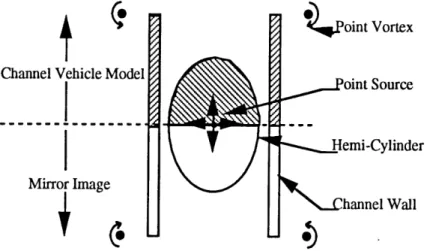
Regardless of the approach used to calculate drag, be it analytical or numerical, one must first be able to effectively model the real flow using an appropriate distribution of the elementary flows presented above. A schematic representation of the model is shown below in Fig. 2.5.

Soint Vortex

Channel Vehicle Model oint Source

Hemi-Cylinder Mirror Image

hannel Wall

Figure 2.5. Schematic of Model for Front-End Drag

The elementary flows which turn out to be crucial to the model for front-end vortex drag are a source flow, and vortical flows. The source flow iteratively simulates penetration, by the vehicle nose, of a fluid slab fixed in the channel guideway. It is able to do this because with each

iteration the source increases in strength , simultaneously forcing greater amounts of fluid out of the channel. When fluid spills out of the channel it is shed off the tips of the guidewalls and thus generates vorticity. Over time, the shed vorticity is pooled into a single vortex, a bow vortex, juxtapositioned to the tip of each guidewall. These real, large-scale vortices are simulated with point vortices. The remaining distribution of singularities in a model depends on the type of solution. In the case of an analytical solution, this is all that is required to simulate front-end drag. However, a numerical solution is not aware of the existence of a nose and guidewalls until these physical entities are constructed geometrically with additional singularities such as vortices. Once all elementary flow have been positioned appropriately, the model is complete and it is possible to proceed with the calculation of drag.

2.2 Analytical Approach to Front-End Vortex Drag

The analytical approach which is pursued in this study does not begin with a simulation which incorporates the full-blown model shown in Fig. 2.5. Instead, a much more basic problem is attacked first to determine the viability of a particular analytical approach to drag. This problem attempts to map the stable shed vortices behind a circular cylinder in a cross-flow to analogous stable positions behind a flat plate in a free stream (see Fig. 1.4). The primary goal of this investigation is to determine the existence, or not, of stable locations for the vortices shed behind the flat plate. If these positions do indeed exist, then the calculation of energy in the flow is straight-forward because the strength of the mapped vortices is known analytically. Furthermore, if this basic problem can be solved, then the full-blown problem can also be solved using a similar mapping technique.

The vortices behind the cylinder have a precise strength, K, which has been calculated by Milne-Thomson [13]. The energy of these vortices is related to their strengths via Batchelor's double summation formula. And, drag is related to energy using a quadruple integral for a general distribution of vorticity [4]. However, this entire procedure for calculating drag is not valid if the vortices behind the flat plate are unstable.

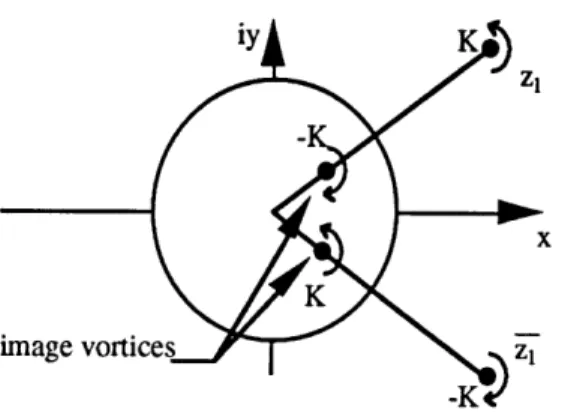
The first step in the mapping problem is to prove that vortices behind the cylinder are indeed stable. This proof must begin with a re-statement of the circle theorem [13]. The circle theorem states that given a point, z, outside a circle of radius 'a' in the imaginary plane and its complex conjugate, z = a2/z, which lies inside the circle, singularities f(z) lie outside the circle and singularities f(a2/z) lie inside the circle. This implies a form for the complex potential, w, which is

w = f(z) + f(). _(2.3) For the problem at hand this means that, in the analytical solution, each vortex outside the cylinder has a vortex of equal but opposite strength inside the cylinder, at a corresponding "inverse" point (i.e. at the point a2_{/z). Thus, the circle theorem provides an analytical tool for the}

construction of a model of vortex shedding behind a circular cylinder in the complex plane. In particular, the flow situation which must be modeled with complex variables is the one in which stationary vortices are positioned behind a circular cylinder.

K

imnage vortices zi -K t

Figure 2.6. Analytical Model for Cylinder with Shed Vorticity

First, consider two vortices located in the complex plane, one at position zi of strength K and the other at position iz of strength -K. The complex potential due only to the presence of these two vortices is iK In( z -zl)/(z - zl). Once a circular cylinder is inserted into the flow, in front of the two vortices, the circle theorem may be invoked to obtain the following expression for the complex potential, w [13].

w = iK In - iK In z -

(2.4) (z-Z) -2

z

If one concentrates on the motion of the vortex at zl and reverses the sense of rotation of each vortex in Fig. 2.6, it is then possible to write the complex potential as w = iK ln(z - zl) + Wz. Here wz is

(z-z-1 (z- a,

z = iK In. - (2.5)

So far, nothing has been said about a cross-flow. That is because, until now, there has not been a need for it in this model. Its presence is required now in order to determine the stable location of the shed vortices. When a cross flow, U, from left to right, parallel to the x-axis in Fig. 2.6, is included, w, becomes

wz = -U(z + ) + iK In z (2.6)

(z _a2

zi

The vortex at zi will be at rest when dwz/dz = 0. Milne-Thomson demonstrated that when the vortices behind the cylinder are stable, it is possible to analytically derive a value for the vortex strength K [13]. Using this value for K, Eq. 2.6 may be differentiated and set equal to zero. Then using the change of variable: z = r exp(iO), 0<08<t/2, it is possible to solve the equation dwz/dz = 0 to obtain the following expression for the position of stable vortices behind a cylinder in a cross-flow:

r2= a2 (2.7)

1 -2 sin 0

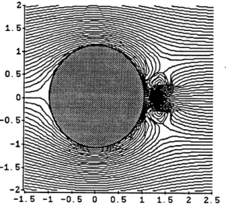
With the help of the symbolic manipulation program Mathematica, it is possible to construct the following visualization of the flow around a cylinder with shed vorticity. Notice that the vortices reside at stable locations behind the cylinder.

0. 5 0. -0.5 -1--2 -1.5 -1 -0.5 0 0.5 1 1.5 2 2.5

The next step is to attempt the mapping of the stable vortices in Fig. 2.7 above to stable positions behind a flat plate. The entire flow pictured above in Fig. 2.7 is mapped from the z-plane, which encompasses the circular cylinder and its two large-scale shed vortices, to the -plane which contains the vertical flat plate and its two large-scale shed vortices (see Fig. 1.4). This is accomplished through the use of the inverse Joukowski transform:

z = 1 ( + 4 a2 ). (2.8)

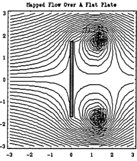
After this transformation has been substituted into Eq. 2.6 and simplified, the mapping is complete. The one peculiarity of the solution is that the mapping is very sensitive to branch cuts. If the branch cuts are not handled carefully, the two vortices inside the cylinder will be mapped to positions outside the flat plate. If care is used in handling the branch cuts, Mathematica once again facilitates the visualization of mapped flow around a flat plate with shed vorticity.

tapped Flow Over A Flat Plate

0

-1

-2

-3

-3 -2 -1 0 1 2 3

Figure 2.8. Simulation of Vorticity Shed behind a Flat Plate

The lingering question concerns the stability of the mapped vortices. In fact, when the vortices are mapped from the z -plane to the C -plane, they seem to acquire an induced velocity because they tend to drift away downstream from the plate. When these mapped vortices are re-mapped some time later to positions behind the circular cylinder, the new positions are no longer stable according to Eq. 2.7. This means that mapping cannot identify stable vortices behind the flat plate. The proposed analytical approach to drag, in this study, is therefore invalid.

However, the outcome of the analytical approach above is not meant to imply that no analytical solution of this problem is possible. In fact the problems with this approach were never fully analyzed. Instead, the decision was made to switch to a simple numerical approach.

One of the most closely related analytical approaches, which does in fact compute drag of vortices shed behind a flat plate, is the inviscid model of vortex shedding developed by Sarpkaya. Sarpkaya begins his analysis by mapping a circular cylinder with shed vortices to an inclined plate with shed vortices. He then imposes the Kutta condition analytically to ensure smooth flow off the tips of the inclined plate. This gives him the strengths of the point vortices closest to the plate tips. He analytically simulates convection of the point vortices and then uses the positions of the convected vortices to formulate a complex potential. Finally, the analytical expression for potential is incorporated into the generalized Blasius theorem to obtain the oscillating drag on a flat plate [14]. Kiya uses similar tactics to solve this problem [10, 11, 12].

2.3 Numerical Approach to Front-End Vortex Drag

The numerical approach is presented in three distinct phases, as noted in chapter 1. The first flow which is simulated is the flow about a circular cylinder in a free stream. Among other things, this simulation is executed to prove that singularities can be used to form the shape of a solid body, such as the nose of a vehicle which moves through a channel guideway. The second simulation addresses the problem of vortex shedding off a flat plate perpendicular to an oncoming free stream. Its purpose is to prove that the vorticity which is shed off the tips of a flat plate in a continuous sheet can be modeled with discrete point vortices. The final simulation incorporates the two previous simulations to model vortex shedding due to the passage of the nose of a flat-bottomed vehicle through a channel guideway.

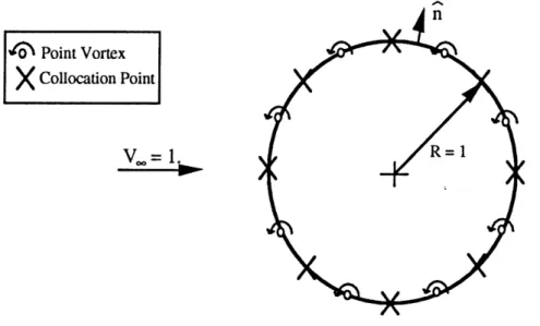
In the problem of a circular cylinder in a free stream, for example, vortices are first arranged in the form of a circle of nondimensional radius, R=1. Then, in this problem as in all the other problems, the numerical scheme is made aware of the existence of an impenetrable barrier by satisfying a flow tangency condition halfway in between each of the fixed vortices (i.e. at the collocation point) around the perimeter of the model for a solid surface. The condition which does this asserts that no fluid shall pass in a direction normal to the line which connects any two vortices positioned to simulate a solid surface. When stated in mathematical terms, it is the following equation.

V*n = 0

V velocity contributions from all vortices at a collocation point. (2.9) n normal vector to a line connecting the two vortices whose

collocation point is the one mentioned above.

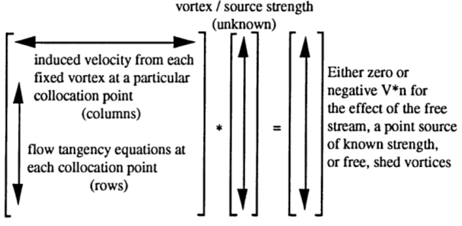
This ensures that the air flow in the numerical simulation does not cross (that is, penetrate) any simulated solid surface formed by the fixed vortices. Once the condition in Eq. 2.9 is applied at each collocation point, it is then possible to form a matrix of flow tangency conditions of the form: A*F = b.

vortex / source strength (unknown) induced velocity from each

fixed vortex at a particular Either zero or

collocation point negative V*n for

(columns) the effect of the free

• = stream, a point source flow tangency equations at of known strength, each collocation point or free, shed vortices

(rows)

Figure 2.9. Solution Matrix for Flow Simulations.

The large, square matrix A is a coefficient matrix which corresponds to variables in the vector F. Each row of A represents the summation of velocities induced by all fixed vortices (of unknown strengths) at a particular collocation point. Each entry in a row of A is a coefficient which represents the velocity contribution of a particular fixed vortex at the collocation point specified by the row in A. Each column of A represents the contribution of a particular fixed vortex to each collocation point. The effect of singularities of known strength is only felt in the right-hand side vector 'b'. The matrix shown in Fig. 2.9 is solved for the unknown strengths, F, and those strengths are used to compute other important flow parameters such as induced velocity and eventually drag, depending on the problem.

Chapter 3

Simulation of Flow over a Circular Cylinder

3.1 Modeling of Flow over a Circular Cylinder

Using the general solution method outlined in chapter 2, it is now possible to discuss individual flow problems, starting with the simulation of flow over a circular cylinder in a free stream. On the surface it seems that this should be a fairly simple and straight-forward problem to solve numerically. After all, the analytical velocity field around a circular cylinder in a free stream may be solved easily using complex variables. See, for example, the book by Anderson [1] for this analytical solution.

V(r,e) = V0 = tangential surface velocity = -2V. sin( ) (3.1)

However, there are some problems with the numerical method which, if not properly addressed, yield an answer with only half the magnitude of the analytical expression in Eq. 3.1.

4 Point Vortex

X

V.= 1. . R

Figure 3.1. Numerical Model for Simulated Flow over a Cylinder.

The simulation is set up, for the most part, as outlined in the previous chapter. Discrete point vortices are first arranged in the shape of a circle of nondimensional radius, R=l. Each point

vortex induces a velocity at a particular collocation point, and the sum of each of those induced velocities constitutes a row of the coefficient matrix, A. Flow tangency equations are then included in the solution matrix, giving a system of 'N' point vortices of unknown strength and 'N' equations written for each collocation point (... an NxN system). Unfortunately, the problem, which is not obvious, with this set up is that the flow tangency equations at one of the collocation points is redundant [5]. One more unknown and an additional equation are required to close the system of equations and solve for the vector 'F'. A point source of unknown strength is placed at the center of the cylinder to bring the total number of unknowns to 'N+I' [7]. The Kutta Condition, which says that flow must leave smoothly off the end of the cylinder, is used as the final, 'N+l'th equation to close the system of (N+1)x(N+1) equations.

3.2 Localized Analytical Correction of Numerical Result

Having constructed the vector equation A*F = b, it is now possible to solve for the strengths of the vortices and point source, and to use these strengths to determine the velocity profile of the fluid flow around the cylinder. The strength of the point source comes out, as expected, to be very small (essentially zero) when the solution matrix is inverted, but it still must be used to close the system of equations. After the matrix equation has been solved for the unknown strengths in the vector F, it is then possible to compute the velocity of fluid on the surface of the cylinder to check the accuracy of the numerical scheme. The numerical answer should be close to the answer in Eq. 3.1. Unfortunately, the numerical scheme encounters problems when trying to evaluate fluid velocities close to the surface of the cylinder. The numerical velocity distribution close to the surface of the cylinder is half the magnitude of the answer determined by the analytical solution.

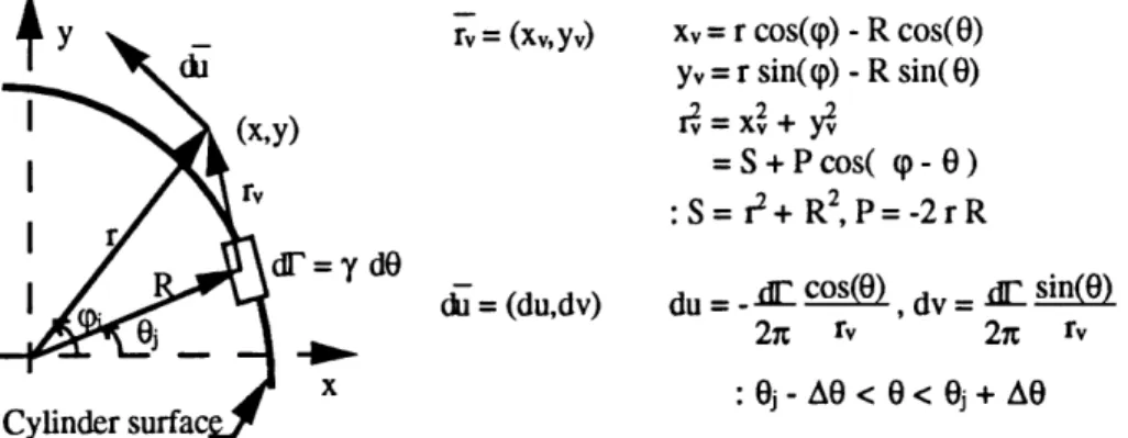
As it turns out, the trick is to use an analytical velocity correction near the cylinder surface (i.e. in the near-field) instead of using the velocity induced by point vortices. The near-field correction is set up by considering a small section of cylinder and smearing the vorticity, F, contained within a near-by point vortex over this section. See Fig. 3.2 below for a model of this type of analytical technique.

y _ rv = (x,yv) Xv= r cos(9) -R cos(0) Ad yv = r sin(q) - R sin(O) (x,y) r = xV + =S+P cos( p - ) r S = r2+ R2, P = -2 r R dr = y dO

Sdu =(du,dv) du= - cos( dv= df sin(0)

92xt rv 2 rv

Cylinder surfac x : 0j - A0 < 0 < 0j + AO

Cylinder surfa

Figure 3.2 Model for Numerical Smoothing Technique

The vertical, near-field velocity induced by the boxed section of vorticity in Fig. 3.2 at point

(x,y) is:

dv = 7Xv y [ rcos q _ Rcos ]dO (3.2) 2t r2_,

2x S+Pcos(9p-0) S+Pcos(9P-0) Using the dummy variable, T, so that T = 0 - (9 and dY = dO,

y rcos p R cosY cos 9 R+ Rsin sin (3.3)

dv = [ _ +si ] (3.3)

2x S+Pcos' S+PcosTF S+Pcos'

Finally, the integration of Eq. 3.3 between 0j - AO - q and 0j + AO - q yields the following expression for the vertical near-field velocity, v.

y R cos

q

)]-R sin In( S + P cos(j + AO - (P)

In( ) ].

P _{S + P cos(Oj - AO - 9)}

y R sin

p

-

)-R sin In( S + P cos(ej + AO - p) P _{S + P cos(0j - AO - 9)}

3.3 Comparison of Analytical and Corrected Numerical Solutions

Using the near-field corrections derived above, it is possible to match the numerical to the analytical fluid velocity profile around the cylinder as shown below in Fig. 3.3. In this graph, r = 1 represents the nondimensional radius of the cylinder, R, and the data shown is with and without smoothing. The data at 81 degrees represents the velocity profile right at a point vortex and the data at 90 degrees is half-way in between vortices. Notice that the rippled data, or data without smoothing, is good far away from the surface of the cylinder (i.e. in the far-field), but not near or on the surface of the cylinder. As mentioned before, the data in between the vortices (at 90

Comparison of Velocity Profiles

results with and without numerical smoothing on a cylinder, R= 1, in afree-stream, U= 1

2.5

2.0 .

1.5 _{....o.... 8ldeg: rippled}

- --- 90deg: rippled # , 90deg: smooth 1.0 ---K--- Analytic soln. 0.5 0.0 • • 1.000 1.125 1.250 1.375 1.500 1.625 1.750 1.875 2.000 Radial Location, r

Figure 3.3. Comparison of Velocity Profiles to Analytical Solution.

degrees) is half the expected value without smoothing, but is effectively equal to the analytical solution when numerical smoothing is performed. Consequently, the numerical scheme with an

analytical correction routine produces the correct flow field for flow about a circular cylinder in a free stream. It can now be inserted into the overall numerical scheme to simulate the cross-section of a vehicle nose which moves through a channel guideway. Modeling of the channel guideway is the subject of chapter 5.

Chapter 4

Simulation of Vortex Shedding behind a Flat Plate

4.1 Modeling of Vortex Shedding behind a Flat Plate

The second flow simulation of interest is the simulation of vortex shedding off a flat plate normal to a free stream. The problem involving the motion of a flat plate through a fluid medium prior to the onset of flow separation off the tips of the plate has been solved analytically using complex variables. However, this problem gets a little more complicated with the introduction of shed vorticity into the flow, justifying the use of numerical methods for a solution. The problem is constructed initially just like the problem of a cylinder in a free stream; fixed point vortices are arranged in such a manner (i.e. in a straight line) that they simulate the surface of a flat plate, perpendicular to a free stream of nondimensional velocity, V. = 1.

ICZ Fixed Point Vortex

'l Free Point Vortex

X

VOO= 1.

Figure 4.1. Numerical Model for Simulated Flow over a Flat Plate.

Initially, all vortices are positioned as shown in Fig. 4.1. A number, N, of fixed vortices are used to simulate the surface of the flat plate while two free vortices lie juxtapositioned to the tips of the plate. Altogether, the 'N+2' vortices, all of unknown strength, simulate a so-called 'extended' flat plate. The 'extended' flat plate, a plate slightly longer than the actual flat plate in the simulation, is a tool which is used to determine the proper location of the two free, near-tip vortices while conserving energy in the flow. This is done by first determining the circulation distribution on the extended flat plate, using the matrix equation A*F = b (see Fig. 2.9).

The circulation distribution is determined using the 'N+2' vortices along with their corresponding 'N+1' collocation points (... and thus 'N+1' equations) halfway in between the vortices and at the plate tips, as shown in Fig. 4.1. The Kutta Condition, which mandates smooth flow off the plate tips, constitutes the N+2nd and final equation. Now, the (N+2)x(N+2) system of equations may be solved for the 'N' unknown fixed vortex strengths and 2 unknown near-tip vortex strengths, F. These strengths represent the strengths of the vortices at the initial time step. The important portion of this circulation distribution is the portion beyond the last collocation point on each end of the flat plate; it is the portion (boxed with hash marks) beyond each tip of the flat plate, as shown in Fig. 4.2. It is important because it locates the appropriate position for each near-tip free vortex by integrating for the 'y' centroid of the portion of the circulation distribution near each plate tip.

X 'y' Centroid:

position of near- Circulation tip free vortex Distribution

V. = 1.--

-Flat Plate

Extended Flat

Plate Tip Region

Figure 4.2. Position of Near-Tip Free Vortices

So far, everything that has been said about the flat plate model has applied only to the initial time step in which there are two free, shed vortices in the flow. However, the same ideas apply to later time steps; the only difference is the existence of more than two free vortices in the flow. Yet, the matrix, A, does not grow in size as additional vortices are shed off the plate tips. It remains a (N+2)x(N+2) matrix. The influence of the so called previously shed vortices, seen in Fig. 4.3, on the solution matrix is seen only in the form of the 'b' vector (see Fig. 2.9). The velocities induced at a particular collocation point by all the previously shed vortices are summed and appear, as a single value, in the form '-V*n' on the right-hand side of the solution matrix, A*F = _{b, where F is now a vector of unknown fixed and near-tip, shed vortex strengths. In}

addition, once free vortices closest to the plate tips are shed into the fluid medium, each free vortex retains its same strength but just changes its location in space during successive shedding iterations. The first pair of shed vortices, for example, retains its same strength throughout

further shedding iterations. vortices.

The only free vortices of unknown strength are the near-tip free

V.= 1.

Figure 4.3. Schematic of Vortex Shedding off a Flat Plate.

4.2 Numerical Vortex Shedding Results and Problems

Once all vortex strengths are known, the induced velocity from each vortex, fixed and free, is computed on each of the free vortices and a new position for each of the free vortices is

Vortex Shedding off a Flat Plate

Numerical Model with Point Sineularities: Drawn to Scale

1.00 0.75 0.50 0.25 0.00 -0.25 -0.50 -0.75 1.00 --1.00 -0.75 -0.50 -0.25 0.00 0.25 0.50 0.75 Flat Plate N Free Vortices 1.00 Horizontal Axis

Figure 4.4. Numerical Results of Vortex Shedding off a Flat Plate

400 Fixed Point Vortex

4\

4 Previously Shed Free Point Vortex

X

it€

0V€-computed according to the integral of the induced velocity. Using a Kutta condition formulated to produce symmetric vortex shedding and adjusting the time scale, the result looks as shown in Fig. 4.4.

A few problems had to be resolved before obtaining the desired solution. First, it was hard to enforce the Kutta condition at both plate tips and still obtain a solution with the geometry shown in Fig. 4.4. The condition of zero circulation, I Fi = 0, which in this case is identical to the Kutta Condition, kept giving a solution with undesired periodic shedding. However, this type of solution is not useful in the larger problem of a vehicle moving through a channel guideway. The larger problem must be able to take advantage of various symmetries in order for it to be tractable. Consequently, the problem of vortex shedding off a flat plate must display some symmetry. This problem was corrected by enforcing top-to-bottom symmetry, via a modified Kutta Condition, in the model shown in Fig. 4.3. When the strengths of the free, shed vortices at opposite edges of the plate are set to be equal in magnitude and opposite in sign, the resultant solution is symmetric, as seen in Fig. 4.4.

One of the most time-consuming issues involves the determination of a geometry for the free vortices. It turns out that the form of the free vortices directly affects the calculation of kinetic energy in the flow. Thus, it is important to select the correct geometry for the free vortices: either with or without cores. When energy is calculated in the Trefftz plane, such as in the problem of vortex shedding behind a wing, it is possible to find the correct size for the cores of free vortices [6]. The result is that the numerical solution, which employs point vortices with cores, is able to match the energy calculated using the more physically valid continuous representation of vorticity in the form of vortex sheets. Sugioka and Kantelis are also able to calculate a vortex core size. But, their problem of vortex shedding behind a circular plate is special because of the cylindrical symmetry involved [9, 15]. Unfortunately, the calculation for energy, in the case of the flat plate, does not occur in the Trefftz plane and the problem does not possess cylindrical symmetry. So it is difficult to obtain a size for the vortex core of a free vortex in this problem, as demonstrated in detail at the beginning of section 4.3. This means that the point vortices in this simulation will be modeled without cores.

4.3 Energy in Vorticity Shed behind a Flat Plate

One method of calculating energy employs vortices of finite size, that is, vortices with cores. When a system of vortices can be simplified down to a pair of vortices with cores, it is possible to derive an analytical expression for the kinetic energy in the flow, as shown below.

Velocity Profile of a finite core vortex Vortex Core

2b= x rc = core radius r

Figure 4.5. Vortex Pair with Cores.

r, 0<rrc

Ve = _(4.1)

,r r< r<oo

Using the integral equation for energy, T:

T = dS (4.2)

The integral in (4.2) is evaluated along a line connecting the centers of the two vortex cores in Fig. 4.5 so that along with the velocity field for a vortex with a finite core, it is possible to express the energy of a vortex pair as

2

T = {n(₂ b - rc _(4.3)

2 r 4 4

The size of the core can now be determined by setting the analytical solution for the energy equal to Eq. 4.3.

rp b2 U2 _p2 - _{b - r ).}

2 2 n r 44)

However, when this is done the core size, re, _{is minuscule and the energy computed using this}

method for successive shedding iterations does not exactly match the expected energy.

The alternate, much simpler method for computing kinetic energy, T, in a flow due to the shedding of vorticity off a flat plate is to use the formula for kinetic energy of a collection of discrete point vortices (i.e. without cores) in space, given by Batchelor [4]:

T=- 4 ]Fi Fj In rij ,(i#j); r, = (Xi - Xj)2 + (Yi - yj)2

ri J _(4.5)

where Ti is the strength of vortex 'i' in the numerical solution.

When this formula is evaluated in the first time step (corresponding to kinetic energy in the flow prior to any shedding of vortices) using a flat plate of semi-span b = 0.5 m, it yields a value of

T/p = 0.321 m4/sec2 for 40 point vortices fixed to a flat plate and T/p = 0.325 m4/sec2 _{for 80}

vortices fixed to the flat plate. This compares fairly well against a value of T/p = 0.393 m4/sec2 from the analytical solution, also derived in Batchelor, with less than a 20% error. One would expect that as the number of vortices fixed to the flat plate approaches infinity, the energy computed using Eq. 4.5 approaches the value for energy obtained from the analytical solution asymptotically. Nevertheless, it was the feeling of this author that the numerical estimate of energy in the flow could be improved upon through the use of clever manipulations of Eq. 4.5 and of the geometry of the flat plate.

The first change that is made to improve the drag estimate is that terms are added to the summation in Eq. 4.5. The terms that are added are terms which calculate the self energy of each discrete vortex. This is like permitting the summation, even when i = j. The problem is that the summation in Eq. 4.5 does not make sense any more when the terms, corresponding to the cases i

= j, are computed as shown. Instead, these terms must be analyzed in integral form. When Eq. 4.5 is expressed in integral form for the case i = j, it assumes the following form for the self energy, Tself.

Tself = ~i

f

In this integral, the circulation of the i th vortex is distributed uniformly over a span Ax for the purpose of calculating Tlf. Integration of Eq. 4.6 yields the following formula for self energy.

Tself _ i (XX)_{self (} 2 _{[2 In (Ax) - 3] (4.7)}

p 8rn

When this equation for self energy is incorporated into the model with 80 vortices, the energy, T/p, obtained is 0.325 m4_/sec2_{, only slightly larger than the 0.321 m}4_/sec2 _{which was obtained}

previously.

The next approach to resolving the discrepancy between the numerical and the analytical solution for energy focuses on accurate description of the circulation and self-energy near the tips of the

plate. In the previous approach, not much thought was given to the circulation distribution near the tips of the plate. In reality, the circulation distribution has a square root singularity near each plate tip. This is seen quite clearly in the circulation distribution from the analytical solution, where 'b' represents the semi-span of the plate [1].

'analytical(X) = k ((x -b)/b) xb

V1 -((x- b)/b)2 (4.8)

The value of the constant kl may be determined by using the circulation given in Eq. 4.8 to integrate for downwash on a plate in a free stream, U = 1. Since the flow around the plate has not yet separated, the downwash is known; it is equal to U. Then the integral equation is

(4.9)

dxl (X - b)2 = I.

1 =~x-x _b2 -

_1x

- b)2

Notice that this is a Cauchy integral. The easiest way to deal with such integrals is to solve them in the complex plane with the appropriate contour. A schematic of the geometry needed to solve such an integral is shown below.

izl

C3

1

C2 A C

.. Flat Plate

Figure 4.6. Path for Cauchy Integration about a Flat Plate.

Now, focus on the [2].

function underneath the square root in Eq. 4.9. It can be evaluated as follows

(x -b)2

b2 ( x _-b) 2

2

i

The integral over the first contour C1is

dxl _/ (X -b) 2

_L

(4.11)

2nRi x 7X b2 _(X 1-b)2

And while the integral over the second contour C2 disappears, the integral over the third contour

C3 becomes

1 dx1 (x1-b) 2 _ i

27tii

Consequently, the function on the left-hand side in Eq. 4.10 is expressed as follows.

(x-b)2 =i+i I (4.13)

b2 - (x- b)2 k 7

When this equation is solved for the real part of I, Re(I), the result is that kl = 2. When this coefficient is substituted into Eq. 4.8, it yields an exact analytical form for the distribution of vorticity over a flat plate. Getting back to the purpose of this analytical approach, the analytical form can now be used to calibrate a square root singularity model for circulation distributions near the plate tips.

Ymodel (x) = k2 (4.14)

The calibration, for a flat plate of semi-span b = 0.5, yields the result k2 = 0.145. Now, since the

circulations at either edge of the plate are not uniform in distribution, the formulation for self-energy must be re-analyzed for the edge point vortices in the flat plate model.

Tself Pi ' ln(x -x2) dx dx2(4.15)

In this integral, the circulation of the i th vortex is set up as a square root type of distribution over a span Ax for the purpose of calculating Tself. After countless changes of variables and integrations, this integration yields the following formula for self energy of the edge vortices.

S _{(Ax)[3-(ln (2)+ 1 In (Ax))] (4.16)}

When this equation is incorporated into the model with 80 vortices, the energy, T/p, obtained is only = 0.327 m4/sec2, which is not much of an improvement. This implies that the self-energy of the vortices on the plate is not as significant as one might think.

The final attempt at resolving the discrepancy between the numerical and the analytical solution for energy focuses on the proper placement of vortices and collocation points near the edges of the plate. Since the placement of vortices and collocation points is very important for the calculation of lift on airfoils in vortex-lattice methods, those placements might also affect energy and drag calculations. Consider the following model of the edge of a plate.

Xl Xcl Xv2 Xc2

I

I

I

0 d 2d x

Figure 4.7. Model of the Edge of a Flat Plate.

The position of the first vortex xvl is determined by finding the centroid of the circulation distribution, which is modeled as a square root singularity, between 0 and d.

xvi dx k 5 dx (4.17)

The solution of this equation yields the vortex position xvl = d/3. A similar integration, between d and 2d, is performed to find the second vortex position xv2.

2d 2d

xv2 k dx= k )K dx (4.18)

The solution of this equation yields the second vortex position xv2 = d (2 i2 - 1)/ (3 (i2- 1)) = 1.5 d. The position of the first collocation point xcl is obtained by equating the downwash y from the continuous distribution at xcl to the downwash induced by the two point vortices at the same collocation point xcl 1

d

kdx d

2dk

dx

.

o

J

dx

(xcl -x)/ (xcl - )1.5 d (4.19)

3 (xcl - 1.5 d)

When this equation is simplified and solved graphically, it turns out that xc = 0.97 d. However, when these new positions are incorporated into the model with 80 vortices, the energy, T/p, remains = 0.327 m4/sec2_{. Unfortunately, time constraints put a stop to this line of investigation.} The discrepancy between the numerical and the analytical solution for energy remains unresolved.

Chapter

5

Simulation of Vortex Shedding from a Channel Guideway

5.1 Modeling of Vortex Shedding with an Expanding Cylinder

The problem of vortex shedding due to the passage of the nose of a vehicle through a channel guideway can be simulated using an expanding cylinder between two parallel walls, with only the upper-half of the model (which will be referred to as the half-model) simulating the actual movement of the vehicle's nose through the channel guideway.

Vortex Drag

+

own Point Source

Model

1(0 Fixed Point Vortex

tej Free Point Vortex

X

Image

Expanding Cylinde Side Wall

Figure 5.1. Schematic of Nose Vortex Drag Model.

That much should be fairly obvious considering the general nose geometry, shown schematically in Fig. 1.3, and the model shown above in Fig. 5.1. What is not obvious is the numerical scheme needed to simulate the real flow out of the channel. In particular, the form of the matrix, A, in the matrix equation A*F = b is not immediately apparent.

The simulation is set up, for the most part, in a manner similar to the general set up outlined in section 2.3. Discrete point vortices are first fixed in the shape of a circle of nondimensional radius, R = 1. In general, there are 'Ncyl' of these vortices with 'Ncyl' collocation points each halfway in between a pair of vortices. The vortices simulate the cross-section of a vehicle nose and its image in the channel guideway. Next, a number, Nwall, of fixed vortices, on each side of

the cylinder, are used to simulate the sidewalls of the channel guideway and their images (see Fig. 5.1). Each sidewall, with its image, has 'Nwall+l' collocation points, each between a pair of fixed vortices and at the tips of the side wall and its image. All vortices in the simulation mentioned thus far are fixed in space and are of unknown strength. There is also one free vortex of unknown strength which lies juxtapositioned to the tip of each side wall and its image, for a total of four near-tip free vortices, also of unknown strengths.

Unfortunately, the simulation of this flow cannot be constructed using a direct superposition of the two numerical schemes used in chapters 3 and 4 (i.e. simulations of a cylinder in a free stream and a flat plate in a free stream). This is due primarily to the absence of a free stream which was present in the other two flow simulations but does not exist in this case. Instead, the source of energy in this simulation is a point source within the cylinder. To first order, the energy of the bow vortices is determined by the source strength, and the vortices fixed to the cylinder have only a second order effect. The main function of these vortices is to preserve the exact shape of the cylinder in the presence of vortices associated with the side walls. Therefore, the problem of the expanding cylinder can be replaced by that of a source between two walls, while still maintaining an excellent approximation to the nose drag.

For the sake of completeness, however, the computation of strength of the vortices on the cylinder shown in Fig. 5.2 is outlined below, even though these vortices are not included in the actual simulation which follows. One immediately encounters the same problem with closure that was encountered for the cylinder in a free stream. The problem can be simplified by introducing symmetry about both the horizontal and vertical axes, i.e. recognize that there is no flow about either the ground plane or the vertical mid-plane. To do this, assume that for each vortex in the first quadrant, there is one of opposite sign in the second quadrant, of the same sign in the third, and of opposite sign in the fourth, all strengths being equal.

The introduction of symmetry eliminates the problem of redundant equations, i.e. the flow-tangency equations satisfy the boundary conditions on the surface of the cylinder and are linearly

Mid-Plane 40\ Fixed Point Vortex

X

2nd quadrant 1st quadran

.Ground Plane

3rd quadrant 4th quadrant

Figure 5.2. Schematic of Cylinder Construction.

independent. However, there is still one more collocation point than vortex, since the boundary conditions must be satisfied at both ends of the quadrant (i.e., there are four X's in Fig. 5.2 and only three O's). This problem is solved by letting the strength of the source at the center be the remaining unknown. Recall that in the case of the cylinder in a free stream, a source was arbitrarily introduced at the center of the cylinder as an unknown and the strength of the source from the numerical solution automatically "came out" to be the right answer, namely zero. Similarly, in the present case, the strength of the source will "come out" to be equal to the rate of change of nose cross-sectional area. To see this, consider the following formula for the source strength.

A Vr r dO = 4 Vr r dO (5.1)

The second integral in Eq. 5.1 is taken along the arc of one quadrant of the cylinder. Now imagine that one wishes to build up the required flow one piece at a time, starting with the expanding cylinder without the plates. We prescribe a velocity Vr at each collocation point. In that case one finds, obviously, that the strength of all the vortices on the surface of the cylinder is zero and A=dA/dt as required. When the vortices on the plates are introduced, they have the same double symmetry as vortices on the cylinder, i.e. no flow through the x-axis or the y-axis, and no net flow across the arc of any quadrant of the cylinder. That is, the local velocities, V,, are affected by the vortices, but the integral is unaffected. Stated differently, we have the following system of equations.