HAL Id: hal-00304722
https://hal.archives-ouvertes.fr/hal-00304722
Submitted on 1 Jan 2002HAL is a multi-disciplinary open access archive for the deposit and dissemination of sci-entific research documents, whether they are pub-lished or not. The documents may come from teaching and research institutions in France or abroad, or from public or private research centers.
L’archive ouverte pluridisciplinaire HAL, est destinée au dépôt et à la diffusion de documents scientifiques de niveau recherche, publiés ou non, émanant des établissements d’enseignement et de recherche français ou étrangers, des laboratoires publics ou privés.
duration curves within ungauged catchments
M. G. R. Holmes, A. R. Young, A. Gustard, R. Grew
To cite this version:
M. G. R. Holmes, A. R. Young, A. Gustard, R. Grew. A region of influence approach to predicting flow duration curves within ungauged catchments. Hydrology and Earth System Sciences Discussions, European Geosciences Union, 2002, 6 (4), pp.721-731. �hal-00304722�
A region of influence approach to predicting flow duration curves
within ungauged catchments
M.G.R. Holmes
1, A.R. Young
1, A. Gustard
1and R. Grew
21Natural Environment Research Council, Centre for Ecology and Hydrology, Wallingford, Oxfordshire, OX10 8BB, UK 2Environment Agency for England and Wales, South West Region, Exeter, EX2 7LQ, UK
Email for corresponding author: [email protected]
Abstract
The development of regionalised hydrological models or procedures for estimating flow duration statistics has been the subject of international research since the 1970s. Historically these models have been based on multivariate statistical models that relate flow statistics to the physical and climatic characteristics of a catchment. The a priori classification of catchments has often been a component of this analysis. This paper discusses the background to the development of such models, with particular emphasis on the United Kingdom; it describes a new region of influence approach to estimating flow duration statistics and compares the performance of this method with current multivariate regression based methods for estimating flow duration statistics within the United Kingdom.
Keywords: hydrological models, regionalisation, river networks, water resources, flow duration curves, region of influence
Introduction
River flow behaviour varies widely across the UK both in space and time. The flashy response of a wet impermeable catchment in the north and west of the country contrasts markedly with that of an English lowland chalk stream, where flows vary little over the year. At the broadest scale, natural river flow regimes are dependent on rainfall, temperature and evaporation. At a local scale, the flows will be controlled by the physical properties of the catchment, including geology, land use and the presence of surface water bodies. Information on the magnitude and variability of flow regimes at the river reach scale is central to aspects of water resources and water quality management. However, many resource assessments are required for ungauged catchments and this has led to the development of a series of regional models for predicting flow statistics within ungauged catchments.
Approaches to the estimation of
natural low flow statistics
International references to techniques for estimating statistics describing the low flow regime at an ungauged
site by models, or rules, relating flow statistics from the same region to physiographic and/or climatic characteristics include Pearson (1995) and Clausen and Pearson (1995) for New Zealand, Musiake et al. (1975) for Japan, Knisel (1963) for south central United States, Mitchell (1957) for Illinois USA, Hines (1975) for Arkansas USA, Klaassen and Pilgrim (1975) and Nathan and McMahon (1992) for Australia, Martin and Cunnane (1976) for Ireland, Lundquist and Krokli (1985) for Norway, and Gustard et al. (1989) for northern and western Europe. Demuth (1993) reviews the regionalisation of low flows in western Europe whilst Smakhtin (2001) provides an extensive review of low flow hydrology, including the estimation of low flows at ungauged sites. Multivariate linear regression analysis is the most widely used statistical technique for developing these models or rules for a region. Linear regression is a special case of Generalised Linear Models (GLM) (Cox and Hinkley, 1974); they are valid only over the range of data set used to construct the models. More sophisticated models involve ascribing a probability distribution to the dependent variable, in this case a flow statistic. Some function, f, known as the link function of the distribution parameters, is then modelled as a linear combination of the independent predictor variables. GLM based techniques for estimating
flow statistics have been used widely in the United States (Stedinger and Tasker, 1985; Kroll and Stedinger, 1998). The definition, or delineation, of homogeneous regions has been the subject of much research both for low flows and flood estimation. In the context of flood estimation, this enables uncorrelated data to be pooled from similar catchments, whilst for low flow estimation the residual variation within a region that has to be explained using a subsequent, multivariate statistical model is normally minimised. A region may be defined by geography, (Institute of Hydrology 1975, 1980), by stream flow characteristics (Wiltshire, 1986; Hughes, 1987; Burn and Boorman, 1993) or by the physical and climatic characteristics of catchments (Acreman and Sinclair, 1986).
The problem with a predefined region approach arises when a new, ungauged catchment is to be assigned to a region. In the case of a geographically based classification, the regions are clearly delineated and the assignment of a catchment is unambiguous. However, in reality, the stream flow characteristics of the catchment may be similar to those for other catchments in more than one region, particularly those that are close to boundaries delineating regions in the vicinity of the ungauged catchment. Furthermore, as the model used for estimating a flow statistic will generally vary between regions, the boundary represents a discontinuity in the estimation of the flow statistics. In the case of a classification based on multivariate stream flow and catchment characteristics, there is commonly a significant overlap between regions. For a classification based on stream flow, the ungauged site will have to be assigned to a region according to the physical and climatic characteristics of the region and the outcome may be erroneous
Using cluster analysis, Burn and Boorman (1993) developed regions, based on streamflow characteristics and subsequently used canonical discriminant analysis to differentiate between regions based on physical and climatic characteristics; this was not entirely satisfactory as the assignment to a region is unambiguous and does not recognise a probability of membership to a region other than that of unity. Acreman and Wiltshire (1989) allowed fractional membership of different regions and averaged the predictions for each region, weighted by the probability of membership of the ungauged site to each. They then dispensed with an a priori definition of region and proposed a dynamic construction of a region based upon the similarity of the characteristics of the gauged catchments to those of the ungauged site. This method, described by Burn (1990a,b) as the region of influence (ROI) for an ungauged site, has been applied to flood estimation by Burn and Zrinji (1994), Robson and Reed (1999) and Burn and Goel (2000).
The history of flow duration curve
estimation in the United Kingdom
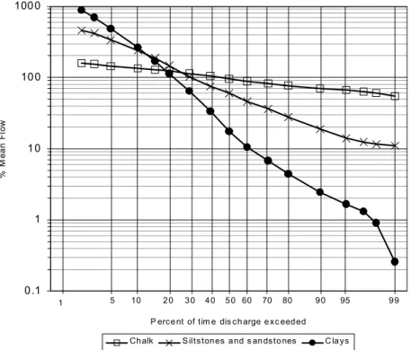
A flow duration curve is an expression of frequency of occurrence; it is constructed from gauged flow data by ranking flows in decreasing order of size and plotting flows as functions of exceedence probability. The curve shows the percentage of time during which any selected discharge may be equalled or exceeded and a log-normal transformation for the flow data is normally applied to linearise the resultant curve. The 1980 Low Flow Studies Report (Institute of Hydrology, 1980), the first major UK study of the relationships between low flow regimes and physiographic and climatic catchment characteristics in the UK, showed that when low flows are expressed as a percentage of the long-term mean flow (standardised), the dependencies on the climatic variability across the country and on the scale effect of catchment area are minimised. The shape of the standardised flow-duration curve indicates the characteristic response of a catchment to rainfall. The gradients of the log-normal flow duration curves for a range of catchments with differing geology (Fig. 1) illustrate that impermeable catchments have high gradient curves reflecting a very variable flow regime; low storage of water in the catchment results in a quick response to rainfall and low flows in the absence of rainfall. Low gradient flow-duration curves indicate that the variance of daily flows is low, because of the damping effects of groundwater storages provided naturally, for example, by extensive chalk or limestone aquifers. This relationship between hydrogeological characteristics and shape is the dominant influence on shape within the UK; thus, approaches to predicting standardised flow duration curves within the UK are targeted largely towards explaining the relationships between shape and catchment hydrogeology.Since the 1980 study for application within the UK, several regional low flow estimation procedures have been developed including those of Pirt and Douglas (1982) and Gustard et al. (1987). Gustard et al. (1992) published the first truly national models for predicting mean flow and flow duration statistics, while Bullock et al. (1994) extended these methods to estimating mean flow and flow duration statistics for specific calendar months. These models were delivered to the user community through a river network based software package Micro LOW FLOWS (Young et al., 2000). All of these methods have been based on multivariate regression analysis. This paper presents a new, region of influence approach to flow duration curve estimation, which builds on the work of Gustard et al. (1992) whose models are referred to as Report 108 procedures.
Report 108 flow duration curve
estimation procedures
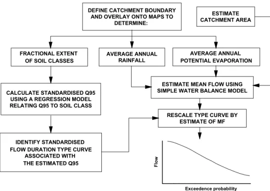
The Report 108 models for predicting flow duration statistics were based on a conceptual water balance model for estimating Mean Flow (MF) and a linear multivariate regression model for predicting the flow equalled or exceeded 95% of the time, standardised by MF (Q95). The estimate of Q95 is used to select a ‘type curve’ from a family of generalised, standardised Flow Duration Curves (FDCs). The resultant flow duration curve is re-scaled by the estimate of MF. The overall estimation procedure is presented as a flow diagram in Fig. 2. These models have been implemented as part of the Micro LOW FLOWS software package (Young et al., 2000) and have been in operational use with UK environmental agencies since the early 1990s. The Report 108 models were developed using the flow records and catchment characteristics for 687 catchments. In the absence of a national digital geology or hydrogeology database of the UK, soil information from the Hydrology Of Soil Types classification (HOST) (mapped at a scale of 1:250,000) was used as a surrogate. HOST is a soil association based hydrological response classification of soils across the United Kingdom (Boorman et al., 1995), and was developed by grouping soil associations into self-similar groups based upon their physical properties which included:
1. Soil hydrogeology using soil descriptions from hydrogeological maps.
2. Depth to aquifer or groundwater. 3. Presence of peaty topsoil.
4. Depth to a slowly permeable layer.
5. Integrated air capacity or “drainable” pore space of a soil layer. A surrogate for permeability in permeable soils and indicative of an impermeable soil’s ability to store excess water.
Thus, although a soils database is used extensively in HOST, the classification does not incorporate hydrogeological data directly. Simple conceptual models describing the flow paths of water provide the structure of the classification scheme. Initially, the 969 UK soil series were analysed and those with similar hydrological response, indicated by their physical properties, were grouped together into a single HOST class. This produced a more manageable data set for further analysis. The percentage cover of the reduced number of classes was then related to gauged Base Flow Index values (Gustard et al., 1992) using multiple regression analysis, as well as by inspection of the response of individual catchments. The regression analysis provided further guidance on discriminating and grouping soil series. The process resulted in a final 30-class system consisting of 29 soil classes and one class representing the fractional extent of lakes. The final form of the classification exists as
0.1 1 10 100 1000 -2.5
P erce nt of tim e dis ch arge e xc eeded
% M e a n F lo w
Chalk S iltstones and s an dsto nes C la ys
10 20 30 40 50 60 70 80 90 95 99
1 5
a set of 1-km digital grids expressing the fractional extent of each HOST class within each 1-km grid cell. Gustard et
al. (1992) used a provisional classification that considered
the dominant HOST class within a 1-km cell.
The Report 108 model developed for predicting standardised Q95 was a multivariate, linear regression model with the dependant variable being Q95 standardised by MF and the 29 HOST classes, amalgamated into 12 Low Flow HOST Groups (LFHGs), forming the independent variables, Eqn. (1).
∑
= × = 1 12 _ 95 i i i LFHG a EST Q (1)where Q95_EST is the estimate of Q95 standardised by MF,
LFHGi is the fraction of Low Flow HOST Group i occurring in the catchment and ai are parameter estimates.
The regression was constrained to have zero intercept, as the fractional extents must sum to unity to resolve the non-independence of fractional extents, as represented by high condition indices within the analysis. The grouping of the HOST classes into the LFHG classes on the basis of similarity in response to rainfall, was required to ensure that realistic parameter estimates could be obtained from the regression analysis. This enabled the issue of poor representation of certain HOST classes, both within the catchment data set and nationally, to be resolved. Grouping
effectively amalgamated poorly represented classes (with parameter estimates that are not significantly different from zero) with better-represented HOST classes, subject to the provisos that the classes could be considered similar in terms of physical properties, and that the addition of the poorly represented class(es) does not modify the parameter estimate unduly for the well represented class. This is equivalent to constraining parameters for poorly represented classes to be equal to the parameter values identified for “similar” classes that are well represented. The primary limitation of the regression model is that the model has difficulty in predicting the extremes within the observed range of Q95 across the data set. Thus, the model tends to over-predict in catchments with low values of standardised Q95 values and under-predict in catchments with high values. This problem of modelling both the extremes of the data and the complete range of data is common to many hydrological modelling activities.
A set of flow duration type curves was used to estimate the full flow duration curve from an estimate of Q95. These curves were derived by pooling standardised curves from 687 catchments using classes defined by equally spaced Q95 values. Operationally, the estimate of Q95 obtained by the multivariate regression model is used to identify appropriate type curves and a FDC that coincides with the predicted value of Q95 is generated by linear interpolation between these curves.
Fig. 2. Procedure for estimating natural flow statistics using the Report 108 methodology DEFINE CATCHMENT BOUNDARY
AND OVERLAY ONTO MAPS TO DETERMINE: FRACTIONAL EXTENT OF SOIL CLASSES AVERAGE ANNUAL RAINFALL AVERAGE ANNUAL POTENTIAL EVAPORATION IDENTIFY STANDARDISED FLOW DURATION TYPE CURVE
ASSOCIATED WITH THE ESTIMATED Q95 CALCULATE STANDARDISED Q95
USING A REGRESSION MODEL RELATING Q95 TO SOIL CLASS
ESTIMATE CATCHMENT AREA
ESTIMATE MEAN FLOW USING SIMPLE WATER BALANCE MODEL
RESCALE TYPE CURVE BY ESTIMATE OF MF
Exceedence probability
Fl
Development of the region of
influence model for estimating flow
duration statistics
The catchment dataset used in the study was based upon a revision of the classification of Gustard et al. (1992), in which all UK gauged catchments were classified according to the hydrometric quality of the gauging station and the impact of water use within the catchment on the ratio of the gauged estimates of Q95 (cumecs) and mean flow. The revision for this study included more recently established stations and considered the absolute impact of artificial influences on the low flow characteristics of the catchment. For this study, 653 gauged catchments were selected with flow records in excess of five years and which were believed to be both relatively natural and of good hydrometric quality. The catchment data set of 653 catchments was subdivided into a calibration data set of 523 catchments for the modelling work and a validation data set of 130 catchments.
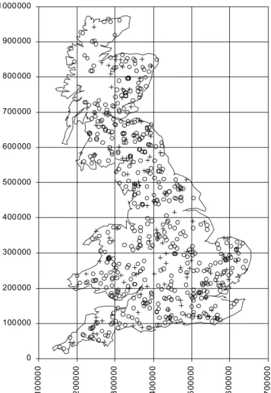
The evaluation catchments were selected randomly from the original data set, so that three ranges of observed Q95 values were represented equally; Q95 < 10%, 10% < Q95 < 20% and Q95 >20%. The distribution of the calibration and evaluation data sets across the UK is shown in Fig. 3. The primary objective in revising the model for predicting standardised Q95 was to reduce the systematic errors at the extremes of the range of Q95. Various approaches were investigated, including additional topographic and climatic catchment characteristics as well as schemes that developed
a priori regions using a geographic and/or data space basis.
The final approach adopted is based on a Region of Influence (ROI) algorithm, developed using the calibration catchment data set and evaluated across both the calibration and evaluation data sets. In developing the new procedures, the potential advantages of standardising for scale effects using the median flow, Q50, and catchment area as alternatives to mean flow were assessed. Standardising by mean flow has the conceptual advantage that the standardising variable can
0 100000 200000 300000 400000 500000 600000 700000 800000 900000 1000000 10 000 0 20 0 0 0 0 30 0 0 0 0 40 0 0 0 0 50 0 0 0 0 60 0 0 0 0 70 0 0 0 0
be estimated from water balance considerations; however, the mean flow is more susceptible to sampling error than the other candidate variables. Standardising by Q50 was found to offer no practical advantages, and left the residual problem of how to estimate Q50 effectively. Standardising by area compromised the ability to predict the standardised flow duration curve effectively. This paper is restricted to describing and comparing the Report 108 and ROI based procedures for estimating standardised flow duration curves. A new approach to estimating mean flow in the United Kingdom, based on a daily-time step soil moisture accounting model, is presented by Holmes et al. (2002). The national, Report 108 Q95 regression model sought to optimise a fit across a wide range of observed values of Q95 by a relatively complex process of minimising the sum-of-squares differences between observed and predicted Q95 using multivariate soil characteristics as predictor variables. The weakness of this approach was that the extremes of the range in Q95 were poorly modelled. The ROI based model reduces the variability of the dependent variable within the data set by reducing it to a much smaller ‘region’ of catchments that are ‘similar’ to the target catchment. An arithmetic, weighted averaging process is then used to predict a value of Q95 for the target catchment from this reduced data set. This approach reduces the within region variability at the expense of the complexity of the predictive model for estimating the flows within the target catchment using the data from the region. The final ROI methodology developed for estimating the full flow duration curve at an ungauged ‘target’ catchment in the UK involves three steps; 1. Catchment similarity is assessed by calculating a weighted Euclidean distance, in HOST space, between the target catchment and every other catchment within a large data pool of natural gauged catchments. 2. A ‘region’ is formed around a target catchment by
ranking all of the catchments in the data pool by their weighted Euclidean distance in HOST space and selecting a set of catchments from the pool that are ‘closest’ to that target catchment.
3. An estimate of Q95 for the target catchment is calculated from a weighted average of the observed Q95 values for the selected catchments in the region, where the weight is based on the reciprocal of the Euclidean distance measure.
For each catchment within the data pool, the weighted Euclidean distance from the target catchment in HOST space is calculated using:
(
)
∑
M m mi− mtit= W X X
de 2 (2)
where deit is the weighted Euclidean distance from the target
catchment, t, to catchment, i, from the data pool; Wm is the weight applied to catchment characteristic, m, and Xmi is the standardised value of catchment characteristic, m, for catchment, i.
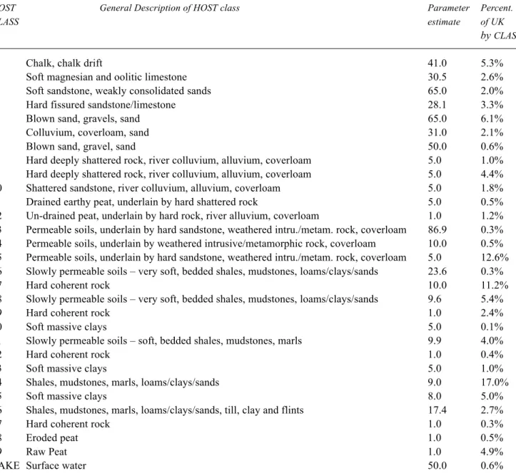
The catchment characteristics, Xm,used are the fractional extents of the 30 HOST classes within a catchment, which will vary between zero and unity. The use of differing weights for individual HOST classes reflects that relatively small proportions of certain HOST classes, especially HOST classes of permeable soil overlying permeable geologies, dominate the variability of the flows within a catchment. The weights were derived using the output from a bounded, multi-variate regression model exercise for predicting Q95 from the fractional extent of HOST classes across the catchments in the calibration scheme and are listed, by HOST class, in Table 1. A region size of ten was ultimately identified as optimal and represented a partially subjective decision based on minimising the unexplained variance across the catchment data set whilst also minimising the tendency for the model to over-predict for very low Q95 catchments and under-predict for very high Q95 catchments. In application, the region of catchments used for estimating Q95 for the target catchment is also used to estimate a standardised flow duration curve for the target. This is estimated by taking a weighted average of the standardised flow duration curves for the gauged catchments within the region, using the same procedure as is used for Q95. This procedure involves weighting each of the ‘n’ catchment’s flow duration curves by the reciprocal distance, in weighted HOST space, of the catchment from the target catchment. Thus, greater weight is given to catchments that are more similar in HOST characteristics to the target catchment. The weighted average estimate for a percentile flow is thus:
(3)
where QP(x)t
PRED is the estimate of the flow for the target
catchment, t, at exceedence percentile P(x); QP(x)i
OBS is the
observed value of QP(x) for the ith source catchment in the region of n (10) catchments closest to the target catchment and deit is the weighted Euclidean distance of the ith catchment from the target catchment, t, in HOST space.
i OBS n i n i it it t PRED QP x de de = x QP ( ) 1 1 ) ( 1 1 5 . 0 5 . 0 ×
∑
∑
= =Table 1. Region of influence weights for individual HOST classes
HOST General Description of HOST class Parameter Percent.
CLASS estimate of UK
by CLASS
1 Chalk, chalk drift 41.0 5.3%
2 Soft magnesian and oolitic limestone 30.5 2.6%
3 Soft sandstone, weakly consolidated sands 65.0 2.0%
4 Hard fissured sandstone/limestone 28.1 3.3%
5 Blown sand, gravels, sand 65.0 6.1%
6 Colluvium, coverloam, sand 31.0 2.1%
7 Blown sand, gravel, sand 50.0 0.6%
8 Hard deeply shattered rock, river colluvium, alluvium, coverloam 5.0 1.0% 9 Hard deeply shattered rock, river colluvium, alluvium, coverloam 5.0 4.4%
10 Shattered sandstone, river colluvium, alluvium, coverloam 5.0 1.8%
11 Drained earthy peat, underlain by hard shattered rock 5.0 0.5%
12 Un-drained peat, underlain by hard rock, river alluvium, coverloam 1.0 1.2% 13 Permeable soils, underlain by hard sandstone, weathered intru./metam. rock, coverloam 86.9 0.3% 14 Permeable soils, underlain by weathered intrusive/metamorphic rock, coverloam 10.0 0.5% 15 Permeable soils, underlain by hard sandstone, weathered intru./metam. rock, coverloam 5.0 12.6% 16 Slowly permeable soils – very soft, bedded shales, mudstones, loams/clays/sands 23.6 0.3%
17 Hard coherent rock 10.0 11.2%
18 Slowly permeable soils – very soft, bedded shales, mudstones, loams/clays/sands 9.6 5.4%
19 Hard coherent rock 1.0 2.4%
20 Soft massive clays 5.0 0.1%
21 Slowly permeable soils – soft, bedded shales, mudstones, marls 9.9 4.0%
22 Hard coherent rock 1.0 0.4%
23 Soft massive clays 5.0 1.0%
24 Shales, mudstones, marls, loams/clays/sands 9.0 17.0%
25 Soft massive clays 8.0 5.0%
26 Shales, mudstones, marls, loams/clays/sands, till, clay and flints 17.4 2.7%
27 Hard coherent rock 1.0 0.3%
28 Eroded peat 1.0 0.5%
29 Raw Peat 1.0 4.9%
LAKE Surface water 50.0 0.6%
Results: estimation of standardised
Q95
The performance indicators adopted were the root mean sum of squares error, RMSE, to give an indication of the random error of the model and the average bias, BIAS. These indicators were calculated as follows;
(
)
∑
= − = n i i PRED i OBS Q Q n RMSE 1 2 95 95 1 (4)∑
= − = n i iOBS i PRED i OBS Q Q Q n BIAS 1 95 95 95 1 (5) where Q95iOBS is the observed Q95 value for catchment i,
Q95i
PRED is the predicted Q95 value for catchment i and n is
the total number of catchments in the data set considered. The performance indicators were evaluated over sub-sets of the calibration and evaluation data sets to examine the performance of the model in low (Q95<10% of mean flow), medium (10%<Q95<20% of mean flow) and high Q95 (Q95>20% of mean flow) catchments. The results are presented in Table 2 for the Report 108 regression model and Table 3 for the ROI model for each Q95 class within both the calibration and evaluation catchment data sets. The performance of the ROI model was evaluated using two
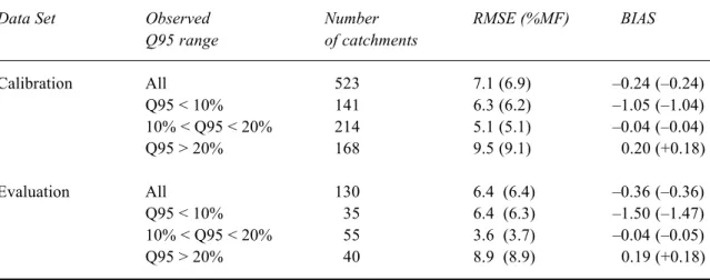
Table 3. Performance of the Region of Influence Q95 model using a data pool of 523 catchments and results
using a data pool of 653 catchments in brackets
Data Set Observed Number RMSE (%MF) BIAS
Q95 range of catchments Calibration All 523 7.1 (6.9) –0.24 (–0.24) Q95 < 10% 141 6.3 (6.2) –1.05 (–1.04) 10% < Q95 < 20% 214 5.1 (5.1) –0.04 (–0.04) Q95 > 20% 168 9.5 (9.1) 0.20 (+0.18) Evaluation All 130 6.4 (6.4) –0.36 (–0.36) Q95 < 10% 35 6.4 (6.3) –1.50 (–1.47) 10% < Q95 < 20% 55 3.6 (3.7) –0.04 (–0.05) Q95 > 20% 40 8.9 (8.9) 0.19 (+0.18)
Table 2. Performance of the Report 108 Q95 model using revised HOST data set
Data Set Observed Number RMSE (%MF) BIAS
Q95 range of catchments Calibration All 523 7.2 –0.28 Q95 < 10% 141 6.7 –1.14 10% < Q95 < 20% 214 5.6 –0.06 Q95 > 20% 168 9.5 0.18 Evaluation All 130 8.0 –0.42 Q95 < 10% 35 6.9 –1.61 10% < Q95 < 20% 55 6.4 –0.10 Q95 > 20% 40 10.4 0.20
different data pools of catchments from which a region could be developed. The first of these was the data pool of the 523 calibration data set catchments used to develop the method. The second data pool was the full data pool of all 653 catchments, the results for which are shown in brackets on Table 3. The results obtained using the full data pool are presented as it is this pool that would be used in practice for estimating at an ungauged site. In this analysis, and in the development of the method, the target catchment was always excluded from the data pool of candidate, source catchments. The performance of the models is illustrated on Fig. 4 for the full data set (653 catchments), using the full data pool of 653 catchments.
Considering first the Report 108 regression model, the data show that the performance of the model over the calibration and evaluation data sets is broadly comparable, with the fit of the calibration set being marginally better than that over the evaluation data set. Over all catchments
within a data set the model BIAS is –0.28 (i.e. a systematic over-prediction error of 28%) over the calibration data set and –0.42 over the evaluation set. This BIAS is primarily a consequence of the over-prediction within low Q95 catchments, although it should be recognised that a large percentage error in these catchments corresponds to a relatively small absolute error. There is a tendency to under-predict within high Q95 catchments, although this is not as marked. The patterns in random error (RMSE) are similar for both catchment data sets. The lowest errors are seen within the middle range of Q95 values and the highest are observed in the highest Q95 range.
The performance of the ROI model (Table 3) is superior to the Existing Report 108 model over all ranges of Q95, both when the data pool is restricted to the calibration data set and when the full data set is used. The systematic and random errors are lower for the ROI model at the extremes of the data set, although some of the differences are small,
and the performance of the model is stable between the calibration and evaluation data set. As expected, the performance of the ROI model improved with an increase in the size of the data pool from which catchments could be drawn.
Results: estimation of standardised
flow duration curve
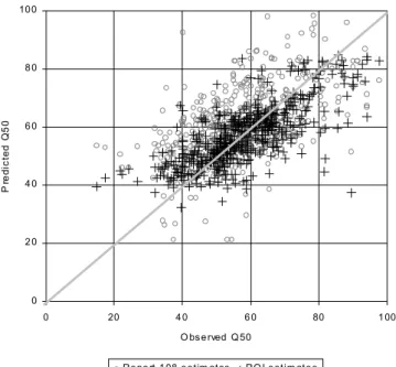
The predictive performance of the ROI based FDC estimation procedure is compared with that of the Report 108 procedure in Figs. 5 and 6 for flows corresponding to two exceedence percentiles; Q(10) and Q(50), respectively. The 1:1 relationship is shown as a line within each plot. These figures demonstrate that the ROI-based estimation of these flows is superior to the use of the type curves and the Report 108 technique.
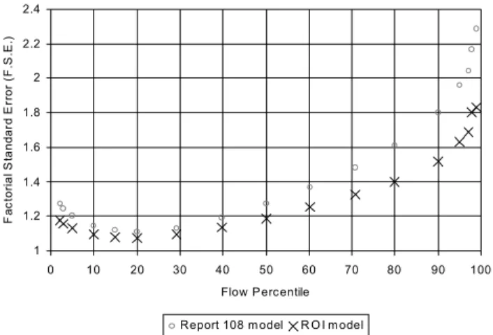
The performance of the two estimation methods was assessed at each of 17, equally spaced, normally transformed points on the flow duration curve by regressing the predicted flow for QxPRED against QxOBS in the following form;
(6) A plot of the factorial standard errors obtained for each percentile point from this regression exercise (Fig. 7) demonstrates that the ROI estimation method is clearly
superior across the entire flow duration curve. As n is large, a 68% prediction confidence interval for a percentile point Q(x) can be approximated as PRED PRED Q x f se Q x e s f x Q ) ( . . ) ( . . ) ( × ≤ ≤ (7) 0 10 20 30 40 50 60 70 0 10 20 30 40 50 60 70 O bse rved Q 95 Pr e d ic te d Q 9 5
Re po rt 108 es tim ates RO I es tim ates
100 120 140 160 180 200 220 240 260 280 300 100 120 140 160 180 200 220 240 260 280 300 O bserved Q 10 Pr e d ic te d Q 1 0
Report 108 es tim ates R OI es tim ates
Fig. 4. A comparison of the predictive capacity of the ROI and
Report 108 models for the Q95 flow percentile
0 2 0 4 0 6 0 8 0 100 0 20 4 0 6 0 80 1 00 O bs e rved Q 50 Pr e d ic te d Q 5 0
Repo rt 1 08 e s tim ates RO I e stim ate s
Fig. 5 . A comparison of the predictive capacity of the ROI and
Report 108 models for the Q10 flow percentile
Fig. 6. A comparison of the predictive capacity of the ROI and
Report 108 models for the Q50 flow percentile
{
}
aOBS
PRED QP x
x
Conclusions
This paper has presented a nationally applicable, region of influence approach to estimating flow duration curves at ungauged sites. Within the approach, a region of hydrogeologically similar catchments is developed using soils data as a surrogate for hydrogeological data. The flow duration data from these catchments are then used to estimate flow duration statistics for the ungauged site. In previous applications of the techniques to the regionalisation of flood events (Burn, 1990a,b; Robson and Reed, 1999) the objective has been to increase the sample size of rare flood events by pooling information from a number of flow records. In this paper, the approach has been used to reduce the variation of flow duration statistics amongst catchments that are subsequently used directly to estimate these statistics for an ungauged catchment.
When tested over a large set of UK catchments, the performance of the new ROI model was superior to that of the Report 108 model, (Gustard et al.,1992) as implemented operationally within the Micro LOW FLOWS software package or applied manually using maps. The Report 108 models are based on a multivariate regression model for predicting Q95 coupled with the selection of a flow duration type curve from a family of such curves. The ROI model reduced both the random and systematic errors across the entire range of flow percentiles. The improvements are attributable to the use of the ROI algorithm dynamically to select a region of ‘similar’ catchments to be used in the estimation of flow statistics. Unlike the Report 108 methods, implemented within Micro LOW FLOWS (Young et al., 2000) or applied manually using maps, the ROI-based models must be used with the re-developed Micro LOW FLOWS software system which incorporates these models
using contemporary programming tools and taking advantage of the increased computing power that is available on the ‘average’ desktop. The UK Environment Agency has implemented the new software, called Low Flows 2000 as a national system.
One weakness of the current formulation of the ROI low flow model is that there is an underlying assumption that the catchment characteristics used to define similarity (the fractional extents of HOST classes) are suitable and sufficient to be used across the entire UK. While these soil parameters may provide strong correlations with flow variability in England and Wales, where the spatial variability in hydrogeology is high, this is not necessarily the case in all parts of the UK. For example, the strong rainfall gradients observed in Scotland may also influence the spatial variability of low flows (Gustard et al., 1987). Furthermore, the HOST classification is used as a surrogate for a nationally consistent hydrogeological classification at a similar or larger scale. The current ROI model uses a fixed ‘region’ size of ten catchments. The choice of ten represents a trade off between minimising the differences between the target catchment and the members of the region, while maximising the differences between the chosen region and the remaining data pool. This effect is most pronounced at the extremes of the range in Q95 observed within the UK. The use of techniques that enable a region to be developed dynamically with additional catchments being included until some measure of within-region similarity is reduced beyond an acceptable limit should be investigated.
This study illustrates that the regionalisation of low flow statistics has come full circle to a point where the concept of a priori regions is dispensed with. The site of interest now forms the centre of a new region that is constructed from observed data using similarity measures specific to low flow hydrology.
Acknowledgements
The research described in this paper was carried out at CEH-Wallingford (formerly the Institute of Hydrology) under funding from the National Environment Research Council and the Environment Agency (Research and Development Project W6-057, Project Manager Dr. Robert Grew).
References
Acreman, M.C. and Wiltshire, S.E., 1989. Regions are dead; long live the regions. Methods of identifying and dispensing with regions for flood frequency analysis. FRIENDS in Hydrology. IAHS Pub. no. 187, 175–188.
1 1.2 1.4 1.6 1.8 2 2.2 2.4 0 10 20 30 40 50 60 70 80 90 100 Flow Percentile F a c to ri a l S ta n da rd E rr o r ( F .S .E .)
Report 108 m odel R O I m odel
Fig. 7. A comparison of the predictive capacity for the Report 108
Acreman, M.C. and Sinclair, C.D., 1986. Classification of drainage basins according to their physical characteristics; an application for flood frequency analysis in Scotland. J. Hydrol., 84, 365– 380.
Boorman, D.B., Hollis, J.M. and Lilly, A., 1995. Hydrology of soil types: a hydrologically – based Classification of the Soils of the United Kingdom. Institute of Hydrology Report 126. Wallingford, UK.
Bullock, A., Gustard, A., Irving, K.M., Sekulin A. and Young, A.R., 1994. Low flow estimation in artificially influenced catchments. National Rivers Authority. R&D Report No. 274. Burn, D.H., 1990a. An appraisal of the “region of influence” approach to flood frequency analysis. Hydrolog. Sci. J., 35, 149– 165.
Burn, D.H., 1990b. Evaluation of regional flood frequency analysis with a region of influence approach. Water Resour. Res., 26, 2257–2265.
Burn, D. H. and Boorman, D. B., 1993. Estimation of hydrological parameters at ungauged catchments. J. Hydrol., 143, 429–454. Burn, D.H. and Goel, N.K., 2000. The formation of groups for regional flood frequency estimation. Hydrolog. Sci. J., 45, 97– 112.
Burn, D.H. and Zrinji, Z., 1994. Flood frequency analysis for ungauged sites using a Region of Influence approach. J. Hydrol.,
153, 1–21.
Clausen, B and Pearson, C.P., 1995. Regional frequency analysis of annual maximum streamflow drought. J. Hydrol., 173, 111– 130.
Cox, D.R. and Hinkley, D.V., 1974. Theoretical Statistics. Chapman and Hall, London.
Demuth, S., 1993. Untersuchungen zum Niedrigwasser in West Europa. Freiburger Schriten zur Hydrologie, Institut fur Hydrologie Band 1, 224pp
Gustard, A., Cole, G.A., Marshall, D.C.W. and Bayliss, A., 1987. A study of compensation flows in the UK. Institute of Hydrology Report 99. Wallingford, UK.
Gustard, A., Roald, L., Demuth, S., Lumadjeng, H. and Gross, R., 1989. Flow regimes from experimental and network data (FREND). 2 Vols. Institute of Hydrology, Wallingford, U.K. Gustard, A., Bullock, A. and Dixon, J.M., 1992. Low Flow
Estimation in the United Kingdom. Institute of Hydrology Report 108. Wallingford, UK.
Hines, M.S., 1975. Flow-duration and low-flow frequency determinations of selected Arkansas streams. USGS Water Resource Circular No. 12.
Holmes, M.G.R., Young, A. R., Grew, R. and Gustard, A., 2002. A new approach to estimating Mean Flow in the United Kingdom. Hydrol. Earth Syst. Sci., 6, 709–720.
Hughes, J.M.R., 1987. Hydrological characteristics and classification of Tasmanian rivers. Aust. Geog. Stud., 25, 61–82. Institute of Hydrology, 1975. Flood Studies Report. Institute of
Hydrology. Wallingford, UK.
Institute of Hydrology, 1980. Low Flow Studies Report. Institute of Hydrology. Wallingford, UK.
Klaassen, B.E. and Pilgrim, D.H., 1975. Hydrograph recession constants for New South Wales streams. Civ. Engng. Trans. Instn. Engrs., Australia, 1975, 43–49.
Knisel, W.G., 1963. Baseflow recession analyses for comparison of drainage basins and geology. J. Geophys. Res., 68, 3649– 3653.
Kroll, C.N. and Stedinger, J.R., 1998. Regional hydrologic analysis: Ordinary and generalized least squares revisited. Water Resour. Res., 34, 121–128.
Lundquist, D. and Krokli, B., 1985. Low Flow Analysis. Norwegian Water Resources and Energy Administration, Oslo. Martin, J.V. and Cunnane, C., 1976. Analysis and prediction of low-flow and drought volumes for selected Irish rivers. The Institution of Engineers of Ireland.
Mitchell, W.D., 1957. Flow duration of Illinois streams. Dept. of Public Works and Buildings, State of Illinois.
Musiake, K., Inokuti, S. and Takahasi, Y., 1975. Dependence of low flow characteristics on basin geology in mountainous areas of Japan. IAHS Publication no. 117, 147–56.
Nathan, R.J. and McMahon, T.A., 1992. Estimating Low Flow Characteristics in Ungauged Catchments. Water Resour. Manage., 6, 85–100.
Pearson, C.P., 1995. Regional Frequency Analysis of Low Flows in New Zealand Rivers. J. Hydrol. (NZ)., 33, 94–122. Pirt, J. and Douglas, R., 1982. A study of low flows using data
from the Severn and Trent catchments. J. Inst. Wat. Engrs Scient., 36, 299–309.
Robson, A. and Reed, D.W., 1999. Statistical Procedures for Flow Frequency Estimation. Flood Estimation Handbook, Vol. 3. Institute of Hydrology, Wallingford.
Smakhtin, V.U., 2001. Low flow hydrology: A review. J. Hydrol.,
240, 147–186.
Stedinger, J.R. and Tasker, G.D., 1985. Regional hydrologic analysis 1. Ordinary, Weighted and Generalized Least Squares Compared. Water Resour. Res., 21, 1421–1432.
Wiltshire, S.E., 1986. Regional Flood Frequency analysis II: Multivariate classification of drainage basins in Britain. Hydrolog. Sci. J., 31, 335–246.
Young, A. R., Gustard, A., Bullock, A., Sekulin, A. E. and Croker, K. M., 2000. A river network based hydrological model for predicting natural and influenced flow statistics at ungauged sites: Micro LOW FLOWS. Sci. Total Environ., 251/252, 293– 304.